
Light Field Video Capture Using a Learning-Based Hybrid Imaging System
Abstract.
Light field cameras have many advantages over traditional cameras, as they allow the user to change various camera settings after capture. However, capturing light fields requires a huge bandwidth to record the data: a modern light field camera can only take three images per second. This prevents current consumer light field cameras from capturing light field videos. Temporal interpolation at such extreme scale (10x, from fps to fps) is infeasible as too much information will be entirely missing between adjacent frames. Instead, we develop a hybrid imaging system, adding another standard video camera to capture the temporal information. Given a fps light field sequence and a standard fps 2D video, our system can then generate a full light field video at fps. We adopt a learning-based approach, which can be decomposed into two steps: spatio-temporal flow estimation and appearance estimation. The flow estimation propagates the angular information from the light field sequence to the 2D video, so we can warp input images to the target view. The appearance estimation then combines these warped images to output the final pixels. The whole process is trained end-to-end using convolutional neural networks. Experimental results demonstrate that our algorithm outperforms current video interpolation methods, enabling consumer light field videography, and making applications such as refocusing and parallax view generation achievable on videos for the first time. Code and data are available at https://cseweb.ucsd.edu/~viscomp/projects/LF/papers/SIG17/lfv/.
1. Introduction
Light field cameras have recently become available in the consumer market (e.g. Lytro), making applications such as post-shot photograph refocusing and viewpoint parallax possible. The great promise of the light-field camera is that a lot of what used to be a pre-process (focus, aperture, etc) can now be a post-process – you shoot first and then decide what you want later. The biggest advantage for this would be for shooting movies, as the director can experiment with changing focus within different parts of the video after it has been captured. It can also save the effort of focus pulling, i.e. manually shifting the focus plane to remain focused on a moving object within a shot.
However, recording scenes in both spatial and angular domains takes a significant amount of data, which limits the maximum data transfer (write) speed, given a limited bandwidth. For example, the raw output image of the Lytro ILLUM camera is pixels, which is nearly times the resolution of 1080p videos. Assuming we are given the same bandwidth as a 1080p fps video, we can only record light field images at fps, which is exactly the rate of the continuous shooting mode for Lytro ILLUM. Although some modern film cameras such as the Red camera (2017) can shoot at higher frame rate, they are usually very expensive, and cannot easily fit the budget for “YouTube filmmakers” – artists making high-quality but low-budget work using consumer-grade equipment and non-traditional distribution channels. For this new democratized cinematography, a $30-50k Red camera is usually out of reach. This makes recording light field videos of normal activities impractical for these artists.
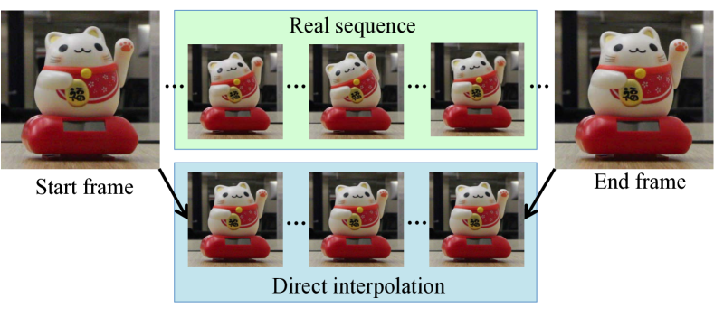
One possible solution is to use a cheaper consumer camera, and perform video interpolation. That is, given the temporal sampling of the scene, interpolate between the input frames to recover the missing frames. However, it is extremely hard to interpolate such a low frame-rate video. In fact, some motion may be entirely missing between neighboring frames, making interpolation impossible, as shown in Fig. 2.
In this paper, we approach this problem in a fundamentally different way. We develop a hybrid imaging system, combining the Lytro ILLUM camera with a video camera capable of capturing a standard fps video (Fig. 1a). The inputs to our system thus consist of a low frame-rate light field video and a standard 2D video (Fig. 1b).111We downsample the video resolution to match the light field sub-aperture resolution. Therefore, the extra bandwidth required for recording the video is actually minimal (about more pixels), and in the future, the two cameras may be merged into one with some hardware modification. The fps light field video captures the angular information, while the fps video gathers the temporal information. Our goal is to output a full light field video with all angular views at the standard video rate (Fig. 1c left). This makes light field image applications achievable on videos for the first time using consumer cameras, such as digital refocusing and parallax view generation as the video is played (Fig. 1c right).
Given the sparse light field sequence and the 2D video, we propose a learning-based approach to combine these two sources of information into one. We achieve this by propagating the angular information captured at the light field frames to the 2D-only frames. For each target view in the missing light field frames, we solve a view synthesis problem. We break down the synthesis process into two steps: a spatio-temporal flow estimation step and an appearance estimation step (Fig. 3). The first step estimates the flows between both the 2D frames and the light field frames, and warps them to the target view accordingly (Sec. 3.1, Fig. 4a). The second step then combines these warped images to output the final pixel color (Sec. 3.2, Fig. 4b).
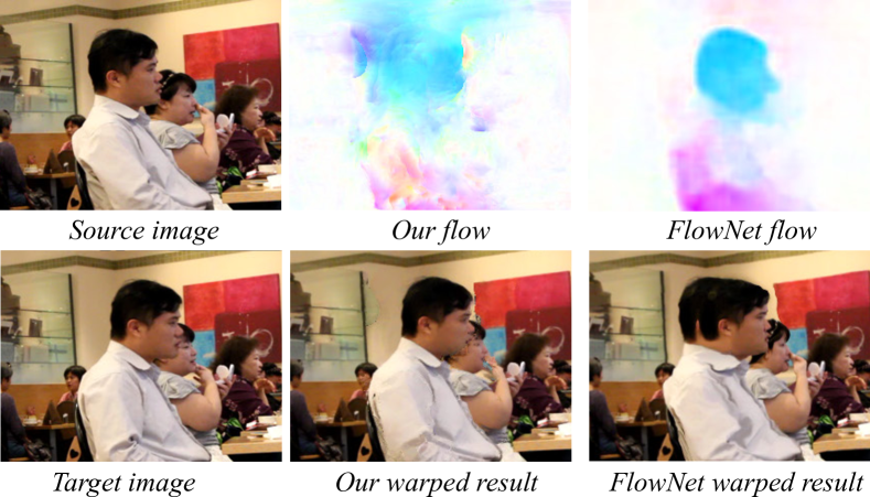
For both estimation steps, we adopt the recently popular convolutional neural network (CNN) (LeCun et al., 1998). An advantage of using CNN methods compared to traditional (i.e. non-learning) methods is that they can provide end-to-end training, so the generated results will usually be better than doing each step independently. Another advantage is that CNNs are much faster than traditional methods. For example, our flow estimation network is two orders of magnitude faster than the state-of-the-art optical flow method (Revaud et al., 2015). Overall, our method takes less than one second to generate a novel view image, and after that, seconds for an additional view. Also note that normally, training flow networks would require the ground truth flows, which are hard to obtain. However, we show that we are able to train them by minimizing errors when the outputs are used to warp images, without utilizing ground truth (Fig. 8).
To better visualize our results, we also develop an interactive user interface to play the resulting light field video, which allows the user to focus to any point as the video plays (Fig. 14), track a given object and remain focused on it throughout the video (Fig. 15), change the (effective) aperture size to create different depths of field (Fig. 16), and vary the viewpoints to provide a more lively viewing experience. Examples of using our interface to achieve these effects can be found in the accompanying video.
In summary, our contributions are:
1) We propose the first algorithm to generate a fps light field video using consumer cameras. Experimental results demonstrate that this cannot be achieved by current state-of-the-art video interpolation and depth from video methods (Figs. 11, 12 and 13).
2) We develop a CNN architecture to combine light field and 2D videos (Figs. 3 and 4). In particular, we train a disparity CNN (Fig. 5a) and an optical flow CNN (Fig. 5b) without utilizing ground truth, and cascade them to combine the angular and the temporal information.
2. Related work
Light Field Video
The origin of light field videos goes back at least to (Wilburn et al., 2002). Nowadays, there are a few devices which can capture a light field video. For example, some high-end models for RayTrix (2017), and the recent Lytro Cinema (2017). However, these devices either have lower spatial or angular resolutions, or are very expensive, and are mainly targeted for research and not for ordinary users. On the other hand, the consumer friendly Lytro ILLUM camera has an affordable price, but is not able to shoot light field videos. In this work, we combine it with an additional 2D camera to interpolate a light field video.
Video Interpolation
Many researchers have tried to upsample the frame rate of 2D videos by interpolating frames in the temporal domain (Mahajan et al., 2009; Baker et al., 2011; Liao et al., 2014; Meyer et al., 2015). However, most existing approaches aim only for slow motion videos, taking a standard 30 fps video as input and trying to generate a very high fps video. This approach, however, is in general not enough to deal with very low fps videos. For a fps video, the motion between neighboring frames is usually very small, which makes interpolation much easier. The same assumption does not hold for a fps video; in fact, some motion may be entirely missing between neighboring frames, making interpolation entirely impossible, as shown in Fig. 2. Moreover, a standard 2D video interpolation method will not produce a consistent light field video for applications like refocusing/viewpoint change, even if applied separately to each view. We show the advantage of our approach over existing 2D interpolation techniques in Sec. 5.
Light Field Super-resolution
Since a light field has a limited resolution, many methods have been proposed to increase its spatial or angular resolution (Bishop et al., 2009; Mitra and Veeraraghavan, 2012; Cho et al., 2013). Some require the input light fields to follow a specific format to reconstruct images at novel views (Levin and Durand, 2010; Marwah et al., 2013; Shi et al., 2014). Wanner and Goldluecke (2014) propose an optimization approach to synthesize new angular views. Yoon et al. (2015) apply convolutional neural networks (CNN) to perform spatial and angular super-resolution. Zhang et al. (2015) propose a phase-based approach to reconstruct light fields using a micro-baseline stereo pair. To synthesize new views, Kalantari et al. (2016) break the problem into depth estimation and appearance estimation and train two sequential neural networks. Wu et al. (2017) apply a CNN-based angular detail restoration on epipolar images to recover missing views. However, none of these methods are designed for temporal upsampling, which is a completely different problem.
Hybrid Imaging System
Combining cameras of two different types to complement each other has also been proposed before. However, they are either used to increase the spatial resolution (Sawhney et al., 2001; Bhat et al., 2007; Boominathan et al., 2014; Wang et al., 2016b, a), deblur the image (Ben-Ezra and Nayar, 2003), or create hyperspectral images (Kawakami et al., 2011; Cao et al., 2011). None of these methods has tried to increase the temporal resolution.
View Synthesis
To synthesize novel views from a set of given images, many methods first estimate the depth and warp the input images to the target view using the obtained depth (Eisemann et al., 2008; Goesele et al., 2010; Chaurasia et al., 2013). The final synthesized image is then a combination of these warped images. To generate a light field video, we also adopt a similar approach. Inspired by (Flynn et al., 2016; Kalantari et al., 2016; Zhou et al., 2016), we use a learning-based approach to perform the geometry and appearance estimations. However, instead of synthesizing images at new viewpoints, we perform image synthesis in the temporal domain.
2D to 3D Conversion
Given a 2D video, there are many works that try to generate the corresponding depth sequence. Konrad et al. (2012) propose a learning-based approach using millions of RGB+depth image pairs, and adopt the k nearest-neighbor (kNN) algorithm to obtain depths for a 2D query video. They then further extend it to predict pixel-wise depth maps by learning a point mapping function from local image/video attributes (Konrad et al., 2013). Karsch et al. (2014) collect an RGBD dataset, and adopt non-parametric depth sampling to generate depths from a monoscopic video based on SIFT flows. However, their method requires the entire training dataset to be available at runtime, which requires significant memory, and is very time consuming. Besides, the above methods only generate depths, while our method can produce a light field sequence.
3. Algorithm


Given a standard ( fps) 2D video and a very low speed light field video (e.g. fps), our goal is to generate a full light field video. Since some of the 2D frames have corresponding light fields (denoted as key frames) while others do not, our main idea is to propagate this multi-view information from these keyframes to the in-between frames. As illustrated in Fig. 3, the overall architecture of our system contains two main parts: spatio-temporal flow estimation CNN and appearance estimation CNN. The spatio-temporal CNN warps the input images from the 2D video and the light field images to the target angular view; the appearance CNN then combines all the warped images to generate a final image. We chose to train neural networks over traditional methods for two reasons. First, using neural networks enables end-to-end training, which typically yields better performance than manually designing each component independently. Second, neural networks usually run times faster than traditional methods.
Note that the light field camera and the video camera will have slightly different viewpoints. For simplicity, we first assume the central view of the light field camera coincides with the 2D video viewpoint. In practice we estimate another flow between the two images to calibrate for that, with more details given in Sec. 4. We also discuss how to handle different color responses between the two cameras in Sec. 4. To make things simpler, we downsample the DSLR resolution to match the Lytro resolution, since spatial super-resolution is not the focus of this paper.
We denote the 2D video frames by and light field sequences by , where is the frame index. Let and be two neighboring keyframes. Our problem can then be formulated as: given and , estimate . We only compute intermediate frames between two adjacent keyframes , and later concatenate all the interpolated results to produce the full video.
3.1. Spatio-temporal flow estimation network
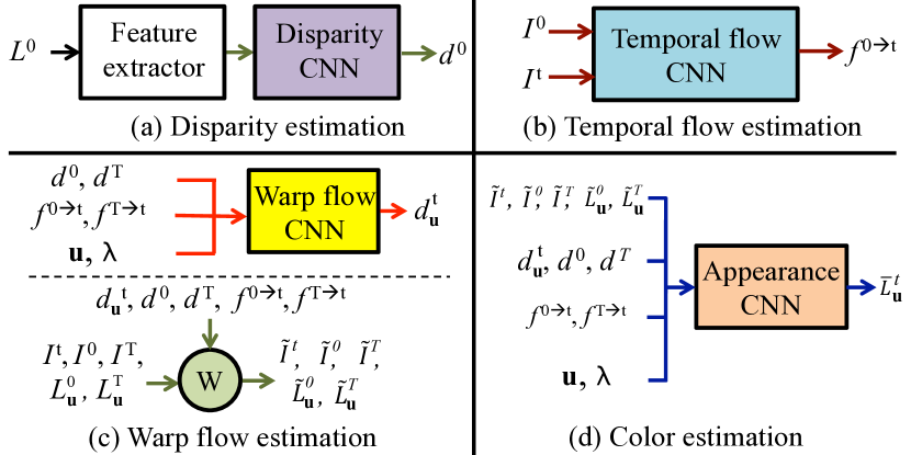
The spatio-temporal flow network can be divided into three components: disparity estimation, temporal flow estimation, and warp flow estimation, as shown in Fig. 4. The first component estimates the disparities at the key frames. The second component (temporal flow estimation) then computes how we can propagate information between the 2D frames. Finally, the third component (warp flow estimation) utilizes the results of the previous two components and propagates disparities to all the 2D frames. We first train each component independently and then end-to-end, along with the appearance estimation network. The inputs and outputs of each component are shown in Fig. 5, and described below. The actual network architectures will be discussed in Sec. 4.
Disparity estimation
Given the light field views of one frame (denoted as or ), we first try to estimate the disparity of this frame at the central view. Our method is similar to the disparity CNN proposed by Kalantari et al. (2016), which is inspired by (Flynn et al., 2016). We briefly introduce the idea here. For each disparity level, we first shift all the views by the corresponding amounts. Ideally, if we shift them by the correct amount, all views will overlap and their mean should be a sharp (in focus) image and their variance should be zero. Therefore, the means and variances of the shifted views are extracted to form a feature map, where is the image size. This process is repeated for different disparity levels, and the features are all concatenated together to form a feature map. This feature is then input to a 4-layer fully convolutional network to generate the depth map.
The only difference of our network from (Kalantari et al., 2016) is that we have all light field views instead of just corner views,222The angular resolution of the Lytro ILLUM is . However, we only use the central views as the views on the border are dark. so we shift all the views accordingly, and take the mean and variance of the shifted views. These shifted images are then put into a CNN to output the disparity at the key frame. In short, the inputs to this network are the views of key frame , and the output is the disparity (Fig. 5a). The same process is performed for the other key frame to obtain .
To train this network, the usual way is to minimize the difference between the output disparity and the ground truth. However, ground truth depths are hard to obtain. Instead, we try to minimize the loss when the output depth is used to warp other views to the central view, which is similar to (Kalantari et al., 2016). In particular, if we assume a Lambertian surface, the relationship between the central view and the other views can be modeled as
| (1) |
where is the spatial coordinate and is the angular coordinate. The loss we try to minimize is then the reconstruction difference (measured by Euclidean distance) between the two sides of (1), summed over all viewpoints,
| (2) |
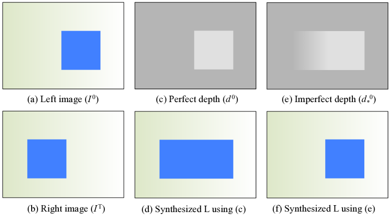
Note that by computing the loss function this way, although we do not have the ground truth depth maps, we are still able to optimize for a functional depth map for the purpose of image synthesis. Also, although we can use methods other than CNN to compute the disparities directly as well, we found that images synthesized by these methods often produce visible artifacts, especially around occlusions. This is because they are not specifically designed for view synthesis. A schematic example is shown in Fig. 6. Note that in this case, a “perfect” depth is actually not able to reconstruct the view around the occlusion boundaries. Instead, a fuzzy depth map will generate a more visually pleasing result. The advantage of using learning-based methods is that although we do not explicitly model occlusions, the network will still try to find some way to handle them.
Temporal flow estimation
We now try to estimate the optical flow between the key frames and the in-between frames in the 2D video. We do this by estimating flows between every pair of neighboring frames in the video, and cascade the flows to get the flow between the key frame and the other frames. Without loss of generality, we consider the case where we estimate the direct flows between two frames and below. The inputs to this network are these two frames. The output is the flow that warps to (Fig. 5b).
Unlike the disparity estimation, this process is much harder for two reasons. First, disparity is a 1D problem, while the general flow is 2D. Second, the pixel displacement in a temporal flow is usually much larger than the case in light fields, so the search range needs to be much larger as well. Based on these conditions, if we use the same architecture as in the previous disparity network, the feature map we extract will have an intractable size. For example, in (Kalantari et al., 2016) each shift amount differs by about 0.4 pixels. If we want to retain the same precision for flows up to pixels, our feature map will be dimensional, which is clearly impractical.
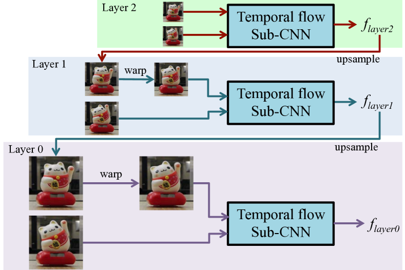
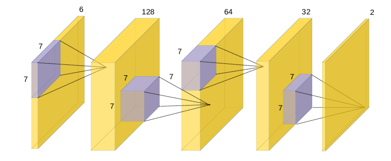
To resolve this, we adopt a hierarchical approach instead (Fig. 7). For the two input frames and , we build a Gaussian pyramid for each of them. Optical flow is then estimated at the coarsest level, and propagated to the finer level below. This process is repeated until we reach the finest level to get the final flow.
Similar to the case of disparity estimation, since ground truth flows are not available, we try to optimize by using the output flow to warp images. More specifically, the relationship between and can be written as
| (3) |
The loss we try to minimize is the Euclidean distance between the two sides of (3),
| (4) |
Note that this is in contrast to other optical flow CNN training procedures such as FlowNet, which requires the ground truth flows.
Warp flow estimation
This step warps the five images shown in Fig. 3 to the target image (missing frame). The five images are: the current 2D frame , the two 2D frames , and two target views , at the keyframes. Note that is usually closer to our final output and often contributes the most, since the angular motion is usually smaller than the temporal motion. However, in some cases the other images will have more impact on the result. For example, when part of the scene is static, will just remain the same throughout the video, so (or ) will be closer to than is to .
To generate the warp flows that warp these images to the target view, we first estimate the disparity at the target view u at the current frame (Fig. 5c up). We do this by utilizing the disparities obtained from key frames and to generate the central view disparity first. To utilize the disparity at key frame , we can first “borrow” its disparity in the same way we borrow its color pixels,
| (5) |
Similarly, we can also borrow the disparity from key frame ,
| (6) |
The final disparity should be somewhere between these two “borrowed” disparities. Intuitively, when we are closer to frame , the current disparity should be closer to , so the weight for it should be higher, and vice versa. We thus add the temporal position as an input to the CNN, indicating this “closeness”
| (7) |
However, since we have no idea how the object depth changes between these two timeframes, there is no simple way to combine the two disparities. Moreover, what we have now is the disparity which warps the target view u to the central view (forward mapping), while we are actually interested in warping the central view to the target view (backward mapping). This is in general very complex and no easy solution exists. Therefore, we try to learn this transformation using a neural network. We thus put the two borrowed disparities and into a CNN to output the final disparity. The output of the network is which satisfies
| (8) |
The loss function of this network is then the Euclidean distance between the two images,
| (9) |
Note that is only available in training data, which are collected using the method described in Sec. 4.2.
Warping
After we obtain the disparity , we are now finished with the estimation part of this step (Fig. 5c up), and can move on to the warping part (Fig. 5c bottom). Note that this part is entirely procedural and does not involve any CNNs. We warp all neighboring images to the missing target view by cascading the flows. For example, let . Then since from (3), we can rewrite (8) as
| (10) |
which warps frame of the 2D video to the current target view.
The above example shows how we can warp one input frame, namely the lower left input image in Fig. 3 to . We denote this warped image as , where the tilde symbol indicates warped images. In the same way, we can also warp the four other input images in Fig. 3, generating five warped images ,, , , and . The warp flows for all the five images are discussed in Appendix A. These five images are then inputs to the next (appearance estimation) neural network to estimate .
3.2. Appearance estimation network
After we warp all the images to the target view, we need to find a way to combine all these images to generate the final output. Existing approaches usually use a simple weighted average to linearly combine them. However, these simple approaches are usually not sufficient to handle cases in which the warped images differ significantly. Instead, we train another network to combine them, inspired by (Kalantari et al., 2016). We stack all five warped images together, along with the disparities and flows we estimated, the target view position u, and the temporal position , and put them into a network to generate the final image (Fig. 5d). The disparities and flows should be useful when detecting occlusion boundaries and choosing different images we want to use. The angular and the temporal positions indicate which images should be weighted more when combining the warped images. Note that unlike (Kalantari et al., 2016), where the input images differ only in the angular domain, here our input images are different in both angular and temporal domains, so the weighting mechanism is even more complex. The final output of the network is the target image. The loss of this network is thus
| (11) |
where is available in the training data. The same procedure is performed for each target view and each time frame to generate the corresponding images.
4. Implementation
We first explain our network architectures in Sec. 4.1, then describe how we train and test our models in Sec. 4.2 and Sec. 4.3.
4.1. Network architecture
For our disparity CNN, the architecture is similar to (Kalantari et al., 2016). For the temporal flow CNN, we adopt a hierarchical approach to estimate the optical flow (Fig. 7). In particular, we first build a pyramid for the two input images. After the flow in the coarsest level is estimated, it is upsampled and used to warp the finer image below. The warped images are then inputs to the network in the next level. This process is repeated until the finest flow is estimated (Fig. 7a). For each layer in the pyramid, the network architectures are the same and are shown in Fig. 7b. For the warp flow CNN and the appearance CNN, the network architectures are similar to the sub-CNN in the temporal flow CNN.
Finally, note that we train our network to generate better final images with an image reconstruction loss function, which is different from previous CNN-based optical flow methods (e.g. FlowNet (Dosovitskiy et al., 2015)). In their cases, the ground truth optical flow is available for networks to directly minimize the flow error. However, we found our approach usually generates more visually pleasing results when warping images, since we are explicitly minimizing the color errors. In particular, in the case of occlusions, the correct flow will actually try to borrow a pixel that is occluded by some other object, resulting in visible artifacts (Fig. 8). Although our flow often looks worse, we are free of this problem by minimizing color errors instead of flow errors.
4.2. Training and Evaluation
We describe how we obtain the ground truth and some details of training our model in this subsection. Upon publication, the source code, the model and the datasets will be released, which will be a useful resource for further research on light field videos.
Ground truth data
To collect training data for our system, we shoot about diverse scenes with slow camera motion or slowly varying object motion using the Lytro ILLUM camera. By collecting data this way, we are able to capture enough temporal information from this “slow motion” light field video as ground truth. Each sequence contains about frames. For each recorded video clip, we treat the first frame and the last frame as keyframes, and the central views of light field images as 2D video frames. We then generate other angular views for the intermediate light field frames via our approach, and compare the generated output with the ground truth data we captured. Example training and test scenes are shown in the supplementary video.
Training details
We now train a network to estimate the light fields for each of the in-between frames in our captured training data. For each training example, we randomly crop the image to extract patches of size . In this way, we have effectively more than 10,000,000 patches for training. We also perform standard data augmentation methods such as randomly scaling the images between and swapping color channels. We initialized the network weights using the MSRA filler (He et al., 2015) and trained our system using the ADAM solver (Kingma and Ba, 2014), with , , and a learning rate of . At every iteration of training, we update the weights of our network using the gradient descent approach. Since each operation of our network is differentiable (convolutions, warpings, etc), computing the gradients can be easily done using the chain rule.
To ease the training difficulty, we first perform stage-wise training of each component in our system, and then perform joint training on all components. This is a common trick to train complex networks (Hinton and Salakhutdinov, 2006).
For the stage-wise training, the losses for the three components of the spatio-temporal flow network are stated in (2), (4) and (9), respectively. After this network is trained, we fix its weights to generate the inputs to the appearance estimation network, and train the appearance estimation network with the loss described in (11).
For joint training, we train both the spatio-temporal flow CNN and the appearance CNN jointly to optimize the cost function defined in (11). This is basically the same as training the appearance CNN only, but allowing the weights in the spatio-temporal flow CNN to change as well. We initialize the weights of each network from what we obtained from stage-wise training. To reduce the memory consumption of joint training, we use a few angular views instead of all the views in the disparity CNN. More training details can be found in Appendix B.
Quantitative Evaluation
To evaluate our method quantitatively, we shot more scenes using the same method (i.e. slow camera motion and object motion) that we used to acquire the training data. We treat this as the test dataset for quantitative evaluation, and compare the image reconstruction error of our method against other previous approaches in Sec. 5.1.
4.3. Testing in real-world scenarios
For real-world scenarios where the “ideal” central view of light field images is inaccessible, we build a prototype in which a DSLR is connected with the Lytro ILLUM via a tripod screw adapter (Fig. 1a). The DSLR records a standard fps 2D video (rotated by degrees), while the Lytro camera captures a fps light field sequence, both of which are used as inputs to our network.
Camera calibration
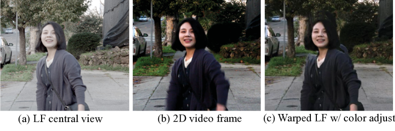
Since the DSLR view does not exactly match the central view of the Lytro camera in terms of viewpoint and color statistics, we first calibrate them by estimating a flow between the two views using non rigid dense correspondence (NRDC) (HaCohen et al., 2011). We chose NRDC due to its robustness to color differences between two cameras. Furthermore, it can output the color transfer function between the two images, so that they can look identical. Figure 9 shows example results before and after the calibration. Finally, to reduce blur in the DSLR image, we always use an aperture of or smaller for the DSLR.
Camera synchronization
Next, to synchronize the images taken with the two cameras, we use the shutter sound the Lytro camera generates when taking images, which is recorded in the video. Typically, there will be roughly to 2D frames between the Lytro camera shots, since the continuous shooting mode does not take images very steadily. Using the sound to dynamically adjust to that gives us better matches than relying on a fixed number.
Testing details
After these two calibrations, the same procedure follows as in the training process except the following differences. First, we downsample the DSLR image to match the Lytro camera resolution. Second, we use all the views in the keyframes rather than randomly sampling views to compute the disparity maps. Finally, we now need to generate all the angular views (including the central view) for each 2D video frame.
5. Results
Below we compare our results both quantitatively (Sec. 5.1) and qualitatively (Sec. 5.2) to other methods, and show applications (Sec. 5.3) and discuss limitations (Sec. 5.4) of our system. A clearer side-by-side comparison and demonstration of our system can be found in the accompanying video. Our system is also significantly faster than other methods, taking less than one second to generate an image. A detailed timing of each stage is described in Sec. 5.1.
5.1. Quantitative comparison
We evaluate our method quantitatively by using the test set described in Sec. 4.2. We compare with direct video interpolation methods and depth from video methods. For video interpolation, we interpolate the light field frames using Epicflow (Revaud et al., 2015) and FlowNet (Dosovitskiy et al., 2015), independently for each viewpoint. Note that they only have the light field frames as input, since there is no easy way to incorporate the high speed video frames into their system. After flows are estimated, the forward warping process is done using the method described in (Baker et al., 2011). For depth from video, we compare with depthTransfer (Karsch et al., 2014), which generates a depth sequence by finding candidates in the training set. Their software also enables production of a stereo sequence using the obtained depths. We thus provide the light field keyframes as training sets, and modify their rendering code to output light fields instead of stereo pairs at each 2D frame. The average PSNR and SSIM values across all in-between frames and the four corner views are reported in Table 1. Our method achieves significant improvement over other methods.
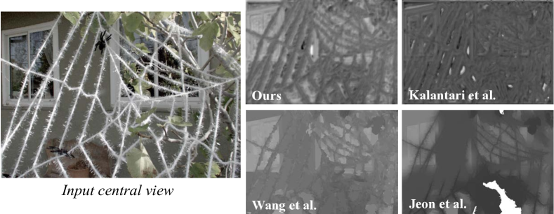
To evaluate the effectiveness of our system, we also try to replace each component in the system by another method. The comparison is shown in Table 2. For the disparity CNN, we replace it with the model in (Kalantari et al., 2016), and two other traditional methods (Jeon et al., 2015; Wang et al., 2015). It can be seen that the traditional methods are not optimized for synthesizing views, so their results are much worse; besides, our method is two to three orders of magnitude faster than these methods. For (Kalantari et al., 2016), although the model is also used for view synthesis, it does not account for temporal flows in the system. In contrast, our system is trained end-to-end with the flow estimation, thus resulting in better performance. A visual comparison of generated depth is shown in Fig. 10. For the temporal flow CNN, we replace it with Epicflow (Revaud et al., 2015) and FlowNet (Dosovitskiy et al., 2015). Although they can in general produce more accurate flows, they are not designed for synthesizing views, so our system still performs slightly better. Also note that our flow network is two orders of magnitude faster than Epicflow. For the warp flow CNN, since no easy substitute can be found, we do not have any comparisons. Finally, for the appearance CNN, we replace it with using only and a weighted average of all warped images. Again, these results are not comparable to our original result, which demonstrates the effectiveness of our appearance CNN.
| Method | Epicflow | FlowNet | DepthTransfer | Ours |
|---|---|---|---|---|
| PSNR | 21.35 | 21.70 | 24.88 | 32.22 |
| SSIM | 0.628 | 0.632 | 0.773 | 0.949 |
| Disparity | Optical flow | Appearance | |||||
|---|---|---|---|---|---|---|---|
| Method | Kalantari | Jeon | Wang | Epicflow | FlowNet | Avg | |
| PSNR | 29.77 | 26.41 | 25.62 | 31.83 | 31.16 | 30.51 | 31.02 |
| SSIM | 0.901 | 0.828 | 0.756 | 0.945 | 0.935 | 0.935 | 0.934 |
Timing
Our method takes seconds to generate a novel view at a particular timeframe, using an Intel i7 3.4 GHz machine with a GeForce Titan X GPU. Specifically, it takes seconds to estimate the disparities, seconds to estimate the temporal flows, seconds to evaluate the warp flow CNN and warp the images, and seconds to evaluate the appearance CNN. Also note that many of these steps (disparity and temporal flow estimations) can be reused when computing different viewpoints, and the parts that require recomputing only take seconds. In contrast, Epicflow takes about seconds ( seconds for computing flows and seconds for warping images using (Baker et al., 2011)), and depthTransfer takes about two minutes. Although flow estimation by FlowNet is fast (around seconds), the subsequent warping process still takes about seconds.
5.2. Qualitative comparison
We visualize the results taken with our prototype (Fig. 1a) qualitatively in this subsection.
Comparison against video interpolation methods
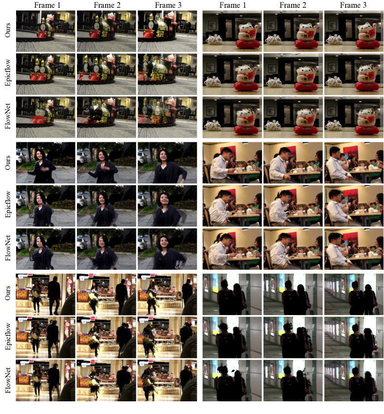
For Epicflow and FlowNet, since these methods cannot easily deal with very low fps inputs, they usually produce temporally inconsistent results, as shown in Fig. 11. For the first scene, we have a toy train moving toward the camera. Note that both Epicflow and FlowNet generate ghosting around the train head, especially as the train is closer so it is moving more quickly. For the lucky cat scene, the body of the cat on the right is swinging. Although optical flow methods can handle the relatively static areas, they cannot deal with the fast moving head and arm of the cat. Next, we have a video of a woman dancing. Again, ghosting effects can be seen around the face and the arms of the woman. Note that in addition to incorrect flows, the ghosting is also partly due to the effect shown in Fig. 6, so the woman appears to have multiple arms. For the dining table scene, the man at the front is acting aggressively, shaking his body and waving his arm. As a result, the other interpolation algorithms fail to produce consistent results. Finally, for the last two scenes, we capture sequences of walking people, with the camera relatively still in the first scene and moving in the second scene. Although the people in general are not moving at a high speed, visible artifacts can still be seen around them.
Comparison against depth from video methods
Comparing with depthTransfer requires more care since it also takes the 2D video as input. In fact, we observe that it usually just copies or shifts the 2D video frames to produce different angular results. Therefore, their results seem to be temporally consistent, but they actually lack the parallax which exists in real light field videos.
To verify the above observation, we first use the test set described in Sec. 4.2, where we have ground truth available. The results of the upper leftmost angular views produced by both our method and depthTransfer are shown in Fig. 12. For each inset, the left column is our result (above) and the error compared to ground truth (bottom), while the right column is the result by depthTransfer and its error. For the first scene, we have a tree and a pole in front of a building. Note that our method realistically reconstructs the structure of the branches. For depthTransfer, since it usually just shifts the scene, although the result may seem reasonable, it lacks the correct parallax so the difference with the ground truth is still large. Next, we have a challenging scene of furry flowers. Note that depthTransfer distorts the building behind and produces artifacts on the flower boundary, while our method can still generate reasonable results. For the bike scene, again depthTransfer distorts the mirror and fails to generate correct parallax for the steering handle. Finally, in the last scene our method realistically captures the shape of the flower and the leaves, while depthTransfer has large errors compared to the ground truth.
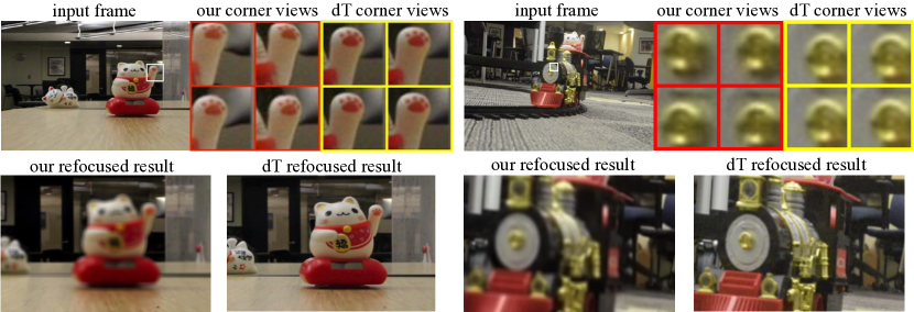
Next, we compare with depthTransfer using the scenes captured with our prototype. Example results are shown in Fig. 13. We show all four corner views at once, so we can see the parallax between different views more easily. It can be seen that results by depthTransfer have very little parallax, while our method generates more reasonable results. This effect is even clearer to see in the refocused images, where results by depthTransfer are actually sharp everywhere. On the other hand, our refocused images have blurry foreground and sharp background.

5.3. Applications
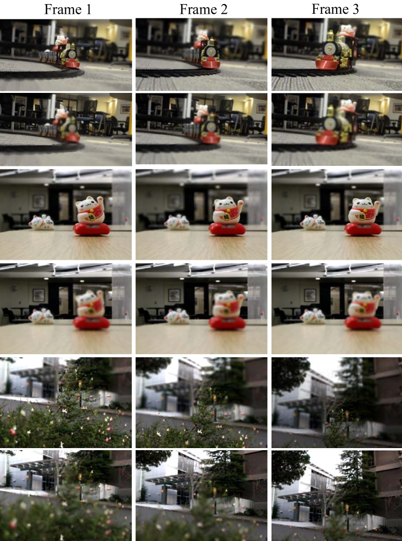
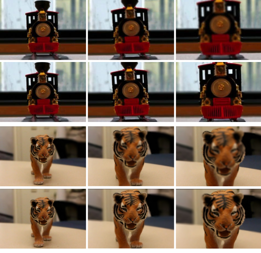
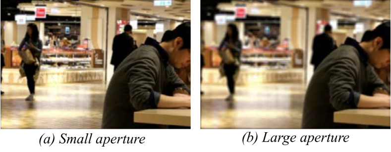
After we obtain the fps light field video, we demonstrate that we are able to do video refocusing. This is useful for changing the focus plane back and forth in a video, or fixing the focus on a particular object no matter where it goes. We also develop an interactive user interface where the user can click on particular points as the video plays, so the point will become in focus. The usage of the interface is shown in the accompanying video, and the results are shown in Fig. 14. In an alternative mode, after the user clicks a point at the start of the video, our algorithm automatically tracks that point using KLT and always focuses on it throughout the video; the results are shown in Fig. 15. Finally, the user can also change the effective aperture to produce different depths of field at each frame, so that does not need to be determined when shooting the video (Fig. 16). All these features are only achievable on light field videos, which are captured and rendered for the first time using consumer cameras by our system.
5.4. Limitations and future work
There are several limitations to our system. First, our results are still not completely artifact-free. We found that artifacts occur mostly around occlusions and are usually caused by improper flow estimation. Since flows between images are undefined in occluded regions, images warped by these flows tend to have some errors in the corresponding regions as well. Our system improves upon current methods by a large margin thanks to end-to-end training, but still cannot solve this problem entirely. An example is shown in Fig. 17. A benefit of our system is that we decompose the pipeline into different components. In the future, if a better flow method is proposed, we can replace that component with such a new method to improve results.

Second, since the Lytro ILLUM camera has a small baseline, the object we try to shoot cannot be too far away. However, if the object is too close, the two views from the Lytro camera and the DSLR become too different and will have large occlusions, making the alignment hard. Therefore, currently our system cannot shoot objects too close or too far away. This can be mitigated by using a smaller attachable camera other than a DSLR, e.g. phone cameras, or having a larger baseline light field camera. Another more fundamental way to deal with this problem is to integrate this into the learning system as well and train end-to-end, so the network can try to infer the difference between the two cameras. This may also save us from running NRDC calibration, which is relatively slow.
Third, if motion blur exists in the videos, the flow estimation will often fail, making the disparity transfer fail. Therefore, currently we ensure the exposure time is low enough that no motion blur occurs. Usually this is easily achievable as long as the scene is not too dark. If capturing a dark scene is inevitable, a possible solution is to deblur the images first. The process can be made easier if we have sharp images from one of the two cameras by using different exposures. This may also make HDR imaging possible.
Next, we do not utilize the extra resolution in the DSLR now. An improvement over our system would be to take that into account and generate a high resolution light field video. We leave this to future work.
6. Conclusion
We propose a novel algorithm to capture a light field video using a hybrid camera system. Although current light field technologies have many benefits, they are mainly restricted to only still images, due to the high bandwidth usage. By incorporating an additional 2D camera to capture the temporal information, we propose a pipeline to combine the 2D video and the sparse light field sequence to generate a full light field video. Our system consists of a spatio-temporal flow CNN and an appearance CNN. The flow CNN propagates the temporal information from the light field frames to the 2D frames, and warps all images to the target view. The appearance CNN then takes in these images and generates the final image. Experimental results demonstrate that our method can capture realistic light field videos, and outperforms current video interpolation and depth from video methods. This enables many important applications on videos, such as dynamic refocusing and focus tracking. We believe this is an important new page for light fields, bringing light field imaging techniques to videography.
Appendix A Concatenation of flows
We show how we warp the five images ,,, and to in this section. In the main text we have already shown how to warp and to get and (by (8) and (10)). We now show how to warp . Let . Then since from (1), we can rewrite (10) as
| (12) | ||||
Similarly, we can write the warp flows for and as
| (13) |
| (14) | ||||
Appendix B Training details
For the end-to-end training, ideally a training example should contain all the images between two key frames and try to output the entire light field sequence. That is, we should have the two light fields (which include and ) and the 2D frames as inputs, and try to output . However, as it is not possible to fit the entire light field sequence into memory during training, each training example only samples some views in the light fields and one frame in the 2D sequence. In particular, instead of using all angular views in the two key frames and , each time we only randomly sample 4 views in addition to the central view . These five views are then used in the disparity estimation network to generate the disparity at the key frames. Similarly, instead of using the central views of all in-between frames, for each training example we only select one frame as input. The flows between the key frames and frame are then estimated using the temporal flow network. This can be seen as angular and temporal “crop,” just as we would randomly crop in the spatial domain during training. For output, we also randomly sample one angular view u at frame . The warp flow network then takes view u and (the central view) at the two key frames, as well as the 2D frame and warps them. Finally the color estimation network takes these warped images and generates the final output. More clearly, the inputs for one training example are: six views ( and u) in the two key frame light fields and , and one 2D frame ( and are just view from and ). The output is one view at frame . The network then tries to minimize the image reconstruction loss (measured by Euclidean distance) between the generated output and .
Acknowledgements
We would like to gratefully thank Manmohan Chandraker and Ren Ng for valuable discussions. This work was funded in part by ONR grant N00014152013, NSF grants 1451830, 1617234 and 1539099, a Google research award, a Facebook fellowship, and the UC San Diego Center for Visual Computing.
References
- (1)
- Baker et al. (2011) Simon Baker, Daniel Scharstein, JP Lewis, Stefan Roth, Michael J Black, and Richard Szeliski. 2011. A database and evaluation methodology for optical flow. International Journal of Computer Vision (IJCV) 92, 1 (2011), 1–31.
- Ben-Ezra and Nayar (2003) Moshe Ben-Ezra and Shree K Nayar. 2003. Motion deblurring using hybrid imaging. In IEEE Conference on Computer Vision and Pattern Recognition (CVPR), Vol. 1. I–657.
- Bhat et al. (2007) Pravin Bhat, C Lawrence Zitnick, Noah Snavely, Aseem Agarwala, Maneesh Agrawala, Michael Cohen, Brian Curless, and Sing Bing Kang. 2007. Using photographs to enhance videos of a static scene. In Eurographics Symposium on Rendering (EGSR). 327–338.
- Bishop et al. (2009) Tom E Bishop, Sara Zanetti, and Paolo Favaro. 2009. Light field superresolution. In IEEE International Conference on Computational Photography (ICCP). 1–9.
- Boominathan et al. (2014) Vivek Boominathan, Kaushik Mitra, and Ashok Veeraraghavan. 2014. Improving resolution and depth-of-field of light field cameras using a hybrid imaging system. In IEEE International Conference on Computational Photography (ICCP). 1–10.
- Cao et al. (2011) Xun Cao, Xin Tong, Qionghai Dai, and Stephen Lin. 2011. High resolution multispectral video capture with a hybrid camera system. In IEEE Conference on Computer Vision and Pattern Recognition (CVPR). 297–304.
- Chaurasia et al. (2013) Gaurav Chaurasia, Sylvain Duchene, Olga Sorkine-Hornung, and George Drettakis. 2013. Depth Synthesis and Local Warps for Plausible Image-based Navigation. ACM Transactions on Graphics (TOG) 32, 3 (2013), 30:1–30:12.
- Cho et al. (2014) Donghyeon Cho, Sunyeong Kim, and Yu-Wing Tai. 2014. Consistent matting for light field images. In European Conference on Computer Vision (ECCV). 90–104.
- Cho et al. (2013) Donghyeon Cho, Minhaeng Lee, Sunyeong Kim, and Yu-Wing Tai. 2013. Modeling the calibration pipeline of the lytro camera for high quality light-field image reconstruction. In IEEE International Conference on Computer Vision (ICCV). 3280–3287.
- Dosovitskiy et al. (2015) Alexey Dosovitskiy, Philipp Fischery, Eddy Ilg, Caner Hazırbaş, Vladimir Golkov, Patrick van der Smagt, Daniel Cremers, and Thomas Brox. 2015. Flownet: Learning optical flow with convolutional networks. In IEEE International Conference on Computer Vision (ICCV). 2758–2766.
- Eisemann et al. (2008) Martin Eisemann, Bert De Decker, Marcus Magnor, Philippe Bekaert, Edilson De Aguiar, Naveed Ahmed, Christian Theobalt, and Anita Sellent. 2008. Floating Textures. Computer Graphics Forum 27, 2 (2008), 409–418.
- Flynn et al. (2016) John Flynn, Ivan Neulander, James Philbin, and Noah Snavely. 2016. DeepStereo: Learning to Predict New Views from the World’s Imagery. In IEEE Conference on Computer Vision and Pattern Recognition (CVPR). 5515–5524.
- Goesele et al. (2010) Michael Goesele, Jens Ackermann, Simon Fuhrmann, Carsten Haubold, Ronny Klowsky, Drew Steedly, and Richard Szeliski. 2010. Ambient point clouds for view interpolation. ACM Transactions on Graphics (TOG) 29, 4 (2010), 95.
- HaCohen et al. (2011) Yoav HaCohen, Eli Shechtman, Dan B Goldman, and Dani Lischinski. 2011. Non-rigid dense correspondence with applications for image enhancement. ACM Transactions on Graphics (TOG) 30, 4 (2011), 70.
- He et al. (2015) Kaiming He, Xiangyu Zhang, Shaoqing Ren, and Jian Sun. 2015. Delving deep into rectifiers: Surpassing human-level performance on imagenet classification. In IEEE International Conference on Computer Vision (ICCV). 1026–1034.
- Hinton and Salakhutdinov (2006) Geoffrey E Hinton and Ruslan R Salakhutdinov. 2006. Reducing the dimensionality of data with neural networks. Science 313, 5786 (2006), 504–507.
- Jeon et al. (2015) Hae-Gon Jeon, Jaesik Park, Gyeongmin Choe, Jinsun Park, Yunsu Bok, Yu-Wing Tai, and In So Kweon. 2015. Accurate depth map estimation from a lenslet light field camera. In IEEE Conference on Computer Vision and Pattern Recognition (CVPR). 1547–1555.
- Kalantari et al. (2016) Nima Khademi Kalantari, Ting-Chun Wang, and Ravi Ramamoorthi. 2016. Learning-based view synthesis for light field cameras. ACM Transactions on Graphics (TOG) 35, 6 (2016), 193.
- Karsch et al. (2014) Kevin Karsch, Ce Liu, and Sing Bing Kang. 2014. DepthTransfer: Depth extraction from video using non-parametric sampling. IEEE Transactions on Pattern Analysis and Machine Intelligence (TPAMI) 36, 11 (2014), 2144–2158.
- Kawakami et al. (2011) Rei Kawakami, Yasuyuki Matsushita, John Wright, Moshe Ben-Ezra, Yu-Wing Tai, and Katsushi Ikeuchi. 2011. High-resolution hyperspectral imaging via matrix factorization. In IEEE Conference on Computer Vision and Pattern Recognition (CVPR). 2329–2336.
- Kingma and Ba (2014) Diederik Kingma and Jimmy Ba. 2014. Adam: A method for stochastic optimization. arXiv preprint arXiv:1412.6980 (2014).
- Konrad et al. (2012) Janusz Konrad, Meng Wang, and Prakash Ishwar. 2012. 2D-to-3D image conversion by learning depth from examples. In IEEE Conference on Computer Vision and Pattern Recognition (CVPR) Workshop. 16–22.
- Konrad et al. (2013) Janusz Konrad, Meng Wang, Prakash Ishwar, Chen Wu, and Debargha Mukherjee. 2013. Learning-based, automatic 2D-to-3D image and video conversion. IEEE Transactions on Image Processing (TIP) 22, 9 (2013), 3485–3496.
- LeCun et al. (1998) Yann LeCun, Léon Bottou, Yoshua Bengio, and Patrick Haffner. 1998. Gradient-based learning applied to document recognition. Proc. IEEE 86, 11 (1998), 2278–2324.
- Levin and Durand (2010) Anat Levin and Fredo Durand. 2010. Linear view synthesis using a dimensionality gap light field prior. In IEEE Conference on Computer Vision and Pattern Recognition (CVPR). 1831–1838.
- Li et al. (2014) Nianyi Li, Jinwei Ye, Yu Ji, Haibin Ling, and Jingyi Yu. 2014. Saliency detection on light field. In IEEE Conference on Computer Vision and Pattern Recognition (CVPR). 2806–2813.
- Liao et al. (2014) Jing Liao, Rodolfo S Lima, Diego Nehab, Hugues Hoppe, Pedro V Sander, and Jinhui Yu. 2014. Automating image morphing using structural similarity on a halfway domain. ACM Transactions on Graphics (TOG) 33, 5 (2014), 168.
- Lytro Cinema (2017) Lytro Cinema. 2017. The ultimate creative tool for cinema and broadcast. https://www.lytro.com/cinema. (2017).
- Mahajan et al. (2009) Dhruv Mahajan, Fu-Chung Huang, Wojciech Matusik, Ravi Ramamoorthi, and Peter Belhumeur. 2009. Moving gradients: a path-based method for plausible image interpolation. ACM Transactions on Graphics (TOG) 28, 3 (2009), 42.
- Marwah et al. (2013) Kshitij Marwah, Gordon Wetzstein, Yosuke Bando, and Ramesh Raskar. 2013. Compressive Light Field Photography Using Overcomplete Dictionaries and Optimized Projections. ACM Transactions on Graphics (TOG) 32, 4 (2013), 46:1–46:12.
- Meyer et al. (2015) Simone Meyer, Oliver Wang, Henning Zimmer, Max Grosse, and Alexander Sorkine-Hornung. 2015. Phase-Based Frame Interpolation for Video. In IEEE Conference on Computer Vision and Pattern Recognition (CVPR). 1410–1418.
- Mitra and Veeraraghavan (2012) Kaushik Mitra and Ashok Veeraraghavan. 2012. Light field denoising, light field superresolution and stereo camera based refocussing using a GMM light field patch prior. In IEEE Conference on Computer Vision and Pattern Recognition (CVPR) Workshop. 22–28.
- RayTrix (2017) RayTrix. 2017. 3D Light Field Camera Technology. https://www.raytrix.de/. (2017).
- Red Camera (2017) Red Camera. 2017. Red Digital Cinema Camera. http://www.red.com/. (2017).
- Revaud et al. (2015) Jerome Revaud, Philippe Weinzaepfel, Zaid Harchaoui, and Cordelia Schmid. 2015. EpicFlow: Edge-preserving interpolation of correspondences for optical flow. In IEEE Conference on Computer Vision and Pattern Recognition (CVPR). 1164–1172.
- Sawhney et al. (2001) Harpreet S Sawhney, Yanlin Guo, Keith Hanna, Rakesh Kumar, Sean Adkins, and Samuel Zhou. 2001. Hybrid stereo camera: an IBR approach for synthesis of very high resolution stereoscopic image sequences. In ACM SIGGRAPH. 451–460.
- Shi et al. (2014) Lixin Shi, Haitham Hassanieh, Abe Davis, Dina Katabi, and Fredo Durand. 2014. Light Field Reconstruction Using Sparsity in the Continuous Fourier Domain. ACM Transactions on Graphics (TOG) 34, 1 (2014), 12:1–12:13.
- Wang et al. (2015) Ting-Chun Wang, Alexei A Efros, and Ravi Ramamoorthi. 2015. Occlusion-aware Depth Estimation Using Light-field Cameras. In IEEE International Conference on Computer Vision (ICCV). 3487–3495.
- Wang et al. (2016b) Ting-Chun Wang, Manohar Srikanth, and Ravi Ramamoorthi. 2016b. Depth from semi-calibrated stereo and defocus. In IEEE Conference on Computer Vision and Pattern Recognition (CVPR). 3717–3726.
- Wang et al. (2016c) Ting-Chun Wang, Jun-Yan Zhu, Ebi Hiroaki, Manmohan Chandraker, Alexei A Efros, and Ravi Ramamoorthi. 2016c. A 4D light-field dataset and CNN architectures for material recognition. In European Conference on Computer Vision (ECCV). 121–138.
- Wang et al. (2016a) Yuwang Wang, Yebin Liu, Wolfgang Heidrich, and Qionghai Dai. 2016a. The Light Field Attachment: Turning a DSLR into a Light Field Camera Using a Low Budget Camera Ring. IEEE Transactions on Visualization and Computer Graphics (TVCG) (2016).
- Wanner and Goldluecke (2014) Sven Wanner and Bastian Goldluecke. 2014. Variational Light Field Analysis for Disparity Estimation and Super-Resolution. IEEE Transactions on Pattern Analysis and Machine Intelligence (TPAMI) 36, 3 (2014), 606–619.
- Wilburn et al. (2002) Bennett Wilburn, Michael Smulski, HH Kelin Lee, and Mark Horowitz. 2002. The light field video camera. In SPIE Proc. Media Processors, Vol. 4674.
- Wu et al. (2017) Gaochang Wu, Mandan Zhao, Liangyong Wang, Qionghai Dai, Tianyou Chai, and Yebin Liu. 2017. Light Field Reconstruction Using Deep Convolutional Network on EPI. In IEEE Conference on Computer Vision and Pattern Recognition (CVPR).
- Yoon et al. (2015) Youngjin Yoon, Hae-Gon Jeon, Donggeun Yoo, Joon-Young Lee, and In So Kweon. 2015. Learning a Deep Convolutional Network for Light-Field Image Super-Resolution. In IEEE International Conference on Computer Vision (ICCV) Workshop. 57–65.
- Zhang et al. (2015) Zhoutong Zhang, Yebin Liu, and Qionghai Dai. 2015. Light field from micro-baseline image pair. In IEEE Conference on Computer Vision and Pattern Recognition (CVPR). 3800–3809.
- Zhou et al. (2016) Tinghui Zhou, Shubham Tulsiani, Weilun Sun, Jitendra Malik, and Alexei A Efros. 2016. View Synthesis by Appearance Flow. In European Conference on Computer Vision (ECCV). 286–301.