Non-negative Matrix Factorization via Archetypal Analysis
Abstract
Given a collection of data points, non-negative matrix factorization (NMF) suggests to express them as convex combinations of a small set of ‘archetypes’ with non-negative entries. This decomposition is unique only if the true archetypes are non-negative and sufficiently sparse (or the weights are sufficiently sparse), a regime that is captured by the separability condition and its generalizations.
In this paper, we study an approach to NMF that can be traced back to the work of Cutler and Breiman [CB94] and does not require the data to be separable, while providing a generally unique decomposition. We optimize the trade-off between two objectives: we minimize the distance of the data points from the convex envelope of the archetypes (which can be interpreted as an empirical risk), while minimizing the distance of the archetypes from the convex envelope of the data (which can be interpreted as a data-dependent regularization). The archetypal analysis method of [CB94] is recovered as the limiting case in which the last term is given infinite weight.
We introduce a ‘uniqueness condition’ on the data which is necessary for exactly recovering the archetypes from noiseless data. We prove that, under uniqueness (plus additional regularity conditions on the geometry of the archetypes), our estimator is robust. While our approach requires solving a non-convex optimization problem, we find that standard optimization methods succeed in finding good solutions both for real and synthetic data.
1 Introduction
Given a set of data points , it is often useful to represent them as convex combinations of a small set of vectors (the ‘archetypes’ ):
| (1.1) |
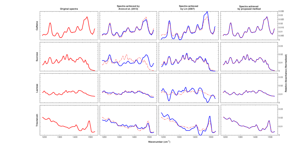
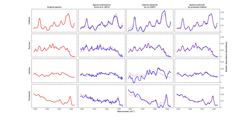
Decompositions of this type have wide ranging applications, from chemometrics [PT94] to image processing [LS99] and topic modeling [XLG03]. As an example, Figure 1 displays the infrared reflection spectra111Data were retrieved from the NIST Chemistry WebBook dataset [LM]. of four molecules (caffeine, sucrose, lactose and trioctanoin) for wavenumber between and . Each spectrum is a vector , with and . If a mixture of these substances is analyzed, the resulting spectrum will be a convex combination of the spectra of the four analytes. This situation arises in hyperspectral imaging [MBDC+14], where a main focus is to estimate spatially varying proportions of a certain number of analytes. In order to mimic this setting, we generated synthetic random convex combinations of the four spectra , …, , each containing two or more of these four analytes, and tried to reconstruct the pure spectra from the ’s. Each column in Figure 1 displays the reconstruction obtained using a different procedure. We refer to Appendix A for further details.
Without further constraints, the decomposition (1.1) is dramatically underdetermined. Given a set of valid archetypes , any set whose convex hull contains the also satisfies Eq. (1.1). For instance, we can set for , and for any , and obtain an equally good representation of the data .
How should we constrain the decomposition (1.1) in such a way that it is generally unique (up to permutations of the archetypes)? Since the seminal work of Paatero and Tapper [PT94, Paa97], and of Lee and Seung [LS99, LS01], an overwhelming amount of work has addressed this question by making the assumptions that the archetypes are componentwise non-negative . Among other applications the non-negativity constraint is justified for chemometrics (reflection or absorption spectra are non-negative), and topic modeling (in this case archetypes correspond to topics, which are represented as probability distributions over words). This formulation has become popular as non-negative matrix factorization (NMF).
Under the non-negativity constraint the role of weights and archetypes becomes symmetric, and the decomposition (1.1) is unique provided that the archetypes or the weights are sufficiently sparse (without loss of generality one can assume ). This point was clarified by Donoho and Stodden [DS03], introduced a separability condition that ensure uniqueness. The non-negative archetypes are separable if, for each there exists an index such that , and for all . If we exchange the roles of weights and archetypes , separability requires that there exists an index such that , and for all This condition has a simple geometric interpretation: the data are separable if for each archetype there is at least one data point such that . A copious literature has developed algorithms for non-negative matrix factorization under separability condition or its generalizations [DS03, AGKM12, RRTB12, AGH+13, GZ15].
Of course this line of work has a drawback: in practice we do not know whether the data are separable. (We refer to the Section 5 for a comparison with [GZ15], which relaxes the separability assumption.) Further, there are many cases in which the archetypes are not necessarily non-negative. For instance, in spike sorting, the data are measurements of neural activity ad the archetypes correspond to waveforms associated to different neurons [RCP09]. In other applications the archetypes are non-negative, but –in order to reduce complexity– the data are replaced by a random low-dimensional projection [KSD08, WL10]. The projected archetypes loose the non-negativity property. Finally, the decomposition (1.1) is generally non-unique, even under the constraint . This is illustrated, again, in Figure 1: all the spectra are strictly positive, and hence we can find archetypes that are still non-negative and whose convex envelope contains .
Since NMF is underdetermined, standard methods fail in such applications, as illustrated in Figure 1 . We represent the data as a matrix whose -th row is the vector , the weights by a matrix and the prototypes by a matrix . The third column of Figure 1 uses a projected gradient algorithm from [Lin07] to solve the problem
| minimize | (1.2) | |||
| subject to |
Empirically, projected gradient converges to a point with very small fitting error , but the reconstructed spectra (rows of ) are inaccurate. The second column in the same figure shows the spectra reconstructed using an algorithm from [AGH+13], that assumes separability: as expected, the reconstruction is not accurate.
In a less widely known paper, Cutler and Breiman [CB94] addressed the same problem using what they call ‘archetypal analysis.’ Archetypal analysis presents two important differences with respect to standard NMF: The archetypes are not necessarily required to be non-negative (although this constraint can be easily incorporated); The under-determination of the decomposition (1.1) is addressed by requiring that the archetypes belong to the convex hull of the data points: .
In applications the condition is too strict. This paper builds on the ideas of [CB94] to propose a formulation of NMF that is uniquely defined (barring degenerate cases) and provides a useful notion of optimality. In particular, we present the following contributions.
Archetypal reconstruction. We propose to reconstruct the archetypes by optimizing a combination of two objectives. On one hand, we minimize the error in the decomposition (1.1). This amounts to minimizing the distance between the data points and the convex hull of the archetypes. On the other hand, we minimize the distance of the archetypes from the convex hull of data points. This relaxes the original condition imposed in [CB94] which required the archetypes to lie in , and allows to treat non-separable data.
Robustness guarantee. We next assume that that the decomposition (1.1) approximately hold for some ‘true’ archetypes and weights , namely , where and captures unexplained effects. We introduce a ‘uniqueness condition’ on the data which is necessary for exactly recovering the archetypes from the noiseless data. We prove that, under uniqueness (plus additional regularity conditions on the geometry of the archetypes), our estimator is robust. Namely it outputs archetypes whose distance from the true ones (in a suitable metric) is controlled by .
Algorithms. Our approach reconstructs the archetypes by minimizing a non-convex risk function . We propose three descent algorithms that appear to perform well on realistic instances of the problem. In particular, Section 4 introduces a proximal alternating linearized minimization algorithm (PALM) that is guaranteed to converge to critical points of the risk function. Appendix E discusses two alternative approaches. One possible explanation for the success of such descent algorithms is that reasonably good initializations can be constructed using spectral methods, or approximating the data as separable, cf. Section 4.1. We defer a study of global convergence of this two-stages approach to future work.
2 An archetypal reconstruction approach
Let be a convex set and , a loss function on . For a point , and a matrix , with rows , we let
| (2.1) | ||||
| (2.2) |
In other words, denoting by the convex hull of the rows of matrix , is the minimum loss between and any point in . If is a matrix with rows , we generalize this definition by letting
| (2.3) |
While this definition makes sense more generally, we have in mind two specific examples in which is actually separately convex in its arguments and . (Most of our results will concern the first example.)
Example 2.1 (Square loss).
In this case , and . This is the case originally studied by Cutler and Breiman [CB94].
Example 2.2 (KL divergence).
We take , the -dimensional simplex, and to be the Kullback-Leibler divergence between probability distributions and , namely .
Given data organized in the matrix , we estimate the archetypes by solving the problem222This problem can have multiple global minima if or in degenerate settings. One minimizer is selected arbitrarily when this happens.
| (2.4) |
where we denote by the set of matrices with rows . A few values of are of special significance. If we set , and , we recover the standard NMF objective (1.2), with a more general distance function . As pointed out above, in general this objective has no unique minimum. If we let after the minimum is evaluated, converges to the minimizer of which is the ‘closest’ to the convex envelope of the data (in the sense of minimizing ). Finally as , the archetypes are forced to lie in and hence we recover the method of [CB94].
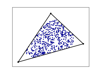
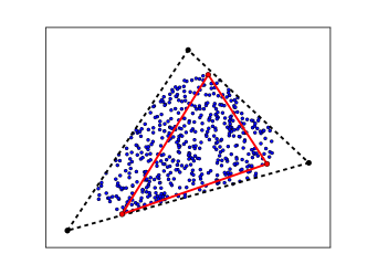
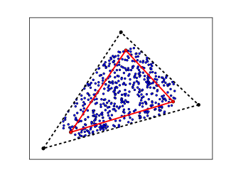
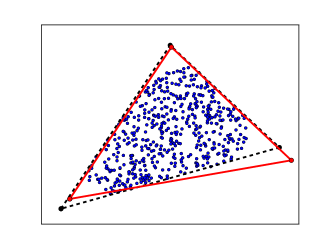
Figure 2 illustrates the advantages of the estimator (2.4) on a small synthetic example, with , , : in this case the data are non separable. We first use the successive projections algorithm of [AGH+13] (that is designed to deal with separable data) in order to estimate the archetypes. As expected, the reconstruction is not accurate because this algorithm assumes separability and hence estimates the archetypes with a subset of the data points. We then use these estimates as initialization in the alternate minimization algorithm of [CB94], which optimizes the objective (2.4) with . The estimates improve but not substantially: they are still constrained to lie in . A significant improvement is obtained by setting to a small value. We (approximately) minimize the cost function (2.4) by generalizing the alternate minimization algorithm, cf. Section 4. The optimal archetypes are no longer constrained to , and provide a better estimate of the true archetypes. The last column in Figure 1 uses the same estimator, and approximately solves problem (2.4) by gradient descent algorithm.
In our analysis we will consider a slightly different formulation in which the Lagrangian of Eq. (2.4) is replaced by a hard constraint:
| minimize | (2.5) | |||
| subject to |
We will use this version in the analysis presented in the next section, and denote the corresponding estimator by .
3 Robustness
In order to analyze the robustness properties of estimator , we assume that there exists an approximate factorization
| (3.1) |
where is a matrix of weights (with rows ), is a matrix of archetypes (with rows ), and we set . The deviation is arbitrary, with rows satisfying . We will assume throughout to be known.
We will quantify estimation error by the sum of distances between the true archetypes and the closest estimated archetypes
| (3.2) |
In words, if is small, then for each true archetype there exists an estimated archetype that is close to it in -loss. Unless two or more of the true archetypes are close to each other, this means that there is a one-to-one correspondence between estimated archetypes and true archetypes, with small errors.
Assumption (Uniqueness).
We say that the factorization satisfies uniqueness with parameter (equivalently, is -unique) if for all with , we have
| (3.3) |
The rationale for this assumption is quite clear. Assume that the data lie in the convex hull of the true archetypes , and hence Eq. (3.1) holds without error term , i.e. . We reconstruct the archetypes by demanding : any such is a plausible explanation of the data. In order to make the problem well specified, we define to be the matrix of archetypes that are the closest to , and hence for all . In order for the reconstruction to be unique (and hence for the problem to be identifiable) we need to assume strictly for . The uniqueness assumption provides a quantitative version of this condition.
Remark 3.1.
Given , , the best constant such that Eq. (3.3) holds for all is a geometric property that depend on only through . In particular, if is a separable factorization, then it satisfies uniqueness with parameter . Indeed in this case , whence and .
It is further possible to show that for all . Indeed, we took to be the matrix of archetypes that are closest to . In other words, and hence, . In addition, since , for an arbitrary row of we have
| (3.4) |
Hence, and therefore
| (3.5) |
Thus, .
We say that the convex hull has internal radius (at least) if it contains an -dimensional ball of radius , i.e. if there exists , , with , such that . We further denote by the condition number of matrix .
Theorem 1.
Assume where the factorization satisfies the uniqueness assumption with parameter , and that has internal radius . Consider the estimator defined by Eq. (2.5), with (square loss) and . If
| (3.6) |
then, we have
| (3.7) |
where is a coefficient that depends uniquely on the geometry of , , namely .
4 Algorithms
While our main focus is on structural properties of non-negative matrix factorization, we provide evidence that the optimization problem we defined can be solved in practical scenarios. A more detailed study is left to future work.
From a computational point of view, the Lagrangian formulation (2.4) is more appealing. For the sake of simplicity, we denote the regularized risk by
| (4.1) |
and leave implicit the dependence on the data . Notice that this function is non-convex and indeed has multiple global minima: in particular, permuting the rows of a minimizer yields other minimizers. We will describe two greedy optimization algorithms: one based on gradient descent, and one on alternating minimization, which generalizes the algorithm of [CB94]. In both cases it is helpful to use a good initialization: two initialization methods are introduced in the next section.
4.1 Initialization
We experimented with two initialization methods, described below.
(1) Spectral initialization. Under the assumption that the archetypes are linearly independent (and for non-degenerate weights ), the ‘noiseless’ matrix has rank exactly . This motivates the following approach. We compute the singular value decomposition , , and initialize as the matrix with rows .
(2) Successive projections initialization. We initialize by choosing archetypes that are a subset of the data , selected as follows. The first archetype is the data point which is farthest from the origin. For each subsequent archetype, we choose the point that is farthest from the affine subspace spanned by the previous ones.
| Archetype initialization algorithm | |
|---|---|
| Input : Data , ; integer ; | |
| Output : Initial archetypes ; | |
| 1: | Set ; |
| 2: | Set ; |
| 3: | For |
| 4: | Define ; |
| 5: | Set ; |
| 6: | Set ; |
| 7: | End For; |
| 8: | Return l |
This coincides with the successive projections algorithm of [ASG+01], with the minor difference that is the affine subspace spanned by the first vectors, instead of the linear subspace333The same modification is also used in [AGH+13], but we do not apply the full algorithm of this paper. This method can be proved to return the exact archetypes if data are separable the archetypes are affine independent [AGH+13, GV14]. When data are not separable it provides nevertheless a good initial assignment.
4.2 Proximal alternating linearized minimization
The authors of [BST14] develop a proximal alternating linearized minimization algorithm (PALM) to solve the problems of the form
| (4.2) |
where and are lower semicontinuous and . PALM is guaranteed to converge to critical points of the function [BST14].
We apply this algorithm to minimize the cost function (4.1), with which we write as
| (4.3) |
where,
| (4.4) | |||
| (4.5) | |||
| (4.6) |
In above equations are the rows of and the indicator function is equal to zero if and is equal to infinity otherwise.
By using this decomposition, the iterations of the PALM iteration reads
| (4.7) | ||||
| (4.8) | ||||
| (4.9) |
where , are step sizes and, for , and a closed convex set, is the matrix obtained by projecting the rows of onto the simplex .
Proposition 4.1.
Consider the risk (4.1), with loss , and the corresponding cost function . If the step sizes are chosen such that , for some constant , then converges to a stationary point of the function .
The proof of this statement is deferred to Appendix D.
It is also useful to notice that the gradient of can be computed explicitly (this can be useful to devise a stopping criterion).
Proposition 4.2.
Consider the risk (4.1), with loss , and assume that the rows of are affine independent. Then, is differentiable at with gradient
| (4.10) | ||||
| (4.11) |
where we recall that denotes the matrix with rows .
The proof of this proposition is given in Appendix C. Appendix E also discusses two alternative algorithms.
4.3 Numerical experiments
We implemented both the PALM algorithm described in the previous section, and the two algorithms described in Appendix E. The outcomes are generally similar.
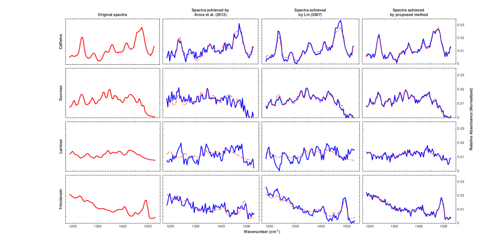
Figures 3 and 4 repeat the experiment already described in the introduction. We generate convex combinations of spectra , , this time adding white Gaussian noise with variance . We minimize the Lagrangian , with444These values were chosen as to approximately minimize the estimation error. (for Figure 3) and (for Figure 4). The reconstructed spectra of the pure analytes appear to be accurate and robust to noise.
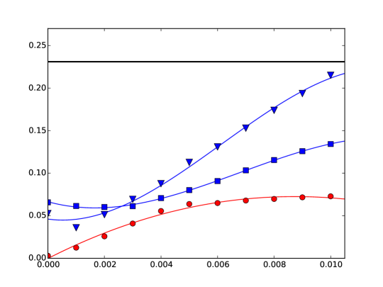
In Figure 5 we repeated the same experiment systematically for noise realizations for each noise level , and report the resulting average loss. Among various reconstruction methods, the approach described in this paper seem to have good robustness to noise and achieves exact reconstruction as .
5 Discussion
We introduced a new optimization formulation of the non-negative matrix factorization problem. In its Lagrangian formulation, our approach consists in minimizing the cost function defined in Eq. (4.1). This encompasses applications in which only one of the factors is required to be non-negative. A special case of this formulation () corresponds to the ‘archetypal analysis’ of [CB94]. In this case, the archetype estimates coincide with a subset of the data points, which is appropriate only under the separability assumption of [DS03].
Our main technical result (Theorem 1) is a robustness guarantee for the reconstructed archetypes. This holds under the uniqueness assumption, which appears to hold for generic geometries of the dataset. In particular, while separability implies uniqueness (with optimal constant ), uniqueness holds for non-separable data as well. To the best of our knowledge, similar robustness results have been obtained under separability [RRTB12, AGH+13, GV14, GV15] (albeit these works obtain a better dependence on ). The only exception is the recent work of Ge and Zou [GZ15] who prove robustness under a ‘subset separability’ condition, which provides a significant relaxation of separability. Under this condition, [GZ15] develops a polynomial-time algorithm to estimate the archetypes by identifying and intersecting the faces of . However, the algorithm of [GZ15] exploits collinearities to identify the faces, and this requires additional ‘genericity’ assumptions.
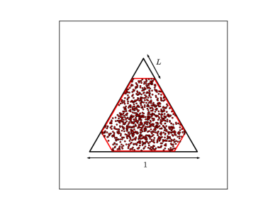
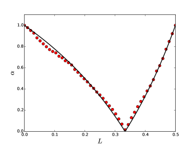
Admittedly, the uniqueness constant is difficult to evaluate analytically, even for simple geometries of the data. However, by definition it does not vanish except in the case of multiple minimizers, and we expect it typically to be of order one. Figure 6 illustrate this point by computing numerically for a simple one-parameter family of geometries with , . The parameter vanishes at a single point, corresponding to a degenerate problem with multiple solutions.
Finally, several earlier works addressed the non-uniqueness problem in classical non-negative matrix factorization. Among others, Miao and Qi [MQ07] penalize a matrix of archetypes by the corresponding volume. Closely related to our work is the approach of Mørup and Hansen [MH12] tha also builds on archetypal analysis. To the best of our knowledge, none of these works establishes robustness of the proposed methods.
We conclude by mentioning three important problems that are not addressed by this paper: Are there natural condition under which the risk function of Eq. (4.1) can be optimized in polynomial time? We only provided an algorithm that is guaranteed to converge to a critical point. We assumed the rank to be known. In practice it will need to be estimated from the data. Similarly, the regularization parameter should be chosen from data.
Acknowledgements
This work was partially supported by the NSF grant CCF-1319979 and a Stanford Graduate Fellowship.
References
- [AGH+13] Sanjeev Arora, Rong Ge, Yonatan Halpern, David M Mimno, Ankur Moitra, David Sontag, Yichen Wu, and Michael Zhu, A practical algorithm for topic modeling with provable guarantees., ICML (2), 2013, pp. 280–288.
- [AGKM12] Sanjeev Arora, Rong Ge, Ravindran Kannan, and Ankur Moitra, Computing a nonnegative matrix factorization–provably, Proceedings of the forty-fourth annual ACM symposium on Theory of computing, ACM, 2012, pp. 145–162.
- [ASG+01] Mário César Ugulino Araújo, Teresa Cristina Bezerra Saldanha, Roberto Kawakami Harrop Galvao, Takashi Yoneyama, Henrique Caldas Chame, and Valeria Visani, The successive projections algorithm for variable selection in spectroscopic multicomponent analysis, Chemometrics and Intelligent Laboratory Systems 57 (2001), no. 2, 65–73.
- [BST14] Jérôme Bolte, Shoham Sabach, and Marc Teboulle, Proximal alternating linearized minimization for nonconvex and nonsmooth problems, Mathematical Programming 146 (2014), no. 1-2, 459–494.
- [CB94] Adele Cutler and Leo Breiman, Archetypal analysis, Technometrics 36 (1994), no. 4, 338–347.
- [DS03] David L Donoho and Victoria Stodden, When does non-negative matrix factorization give a correct decomposition into parts?
- [GV14] Nicolas Gillis and Stephen A Vavasis, Fast and robust recursive algorithmsfor separable nonnegative matrix factorization, IEEE transactions on pattern analysis and machine intelligence 36 (2014), no. 4, 698–714.
- [GV15] , Semidefinite programming based preconditioning for more robust near-separable nonnegative matrix factorization, SIAM Journal on Optimization 25 (2015), no. 1, 677–698.
- [GZ15] Rong Ge and James Zou, Intersecting faces: Non-negative matrix factorization with new guarantees, Proceedings of the 32nd International Conference on Machine Learning (ICML-15), 2015, pp. 2295–2303.
- [KSD08] Dongmin Kim, Suvrit Sra, and Inderjit S Dhillon, Fast projection-based methods for the least squares nonnegative matrix approximation problem, Statistical Analysis and Data Mining 1 (2008), no. 1, 38–51.
- [Lin07] Chih-Jen Lin, Projected gradient methods for nonnegative matrix factorization, Neural computation 19 (2007), no. 10, 2756–2779.
- [LM] P.J. Linstrom and W.G. Mallard (eds.), Nist chemistry webbook, nist standard reference database number 69, National Institute of Standards and Technology, Gaithersburg MD, 20899, http://webbook.nist.gov, (retrieved January 5, 2017).
- [LS99] Daniel D Lee and H Sebastian Seung, Learning the parts of objects by non-negative matrix factorization, Nature 401 (1999), no. 6755, 788–791.
- [LS01] , Algorithms for non-negative matrix factorization, Advances in neural information processing systems, 2001, pp. 556–562.
- [MBDC+14] Wing-Kin Ma, José M Bioucas-Dias, Tsung-Han Chan, Nicolas Gillis, Paul Gader, Antonio J Plaza, ArulMurugan Ambikapathi, and Chong-Yung Chi, A signal processing perspective on hyperspectral unmixing: Insights from remote sensing, IEEE Signal Processing Magazine 31 (2014), no. 1, 67–81.
- [MH12] Morten Mørup and Lars Kai Hansen, Archetypal analysis for machine learning and data mining, Neurocomputing 80 (2012), 54–63.
- [MN13] Boris S Mordukhovich and Nguyen Mau Nam, An easy path to convex analysis and applications, Synthesis Lectures on Mathematics and Statistics 6 (2013), no. 2, 1–218.
- [MQ07] Lidan Miao and Hairong Qi, Endmember extraction from highly mixed data using minimum volume constrained nonnegative matrix factorization, IEEE Transactions on Geoscience and Remote Sensing 45 (2007), no. 3, 765–777.
- [Paa97] Pentti Paatero, Least squares formulation of robust non-negative factor analysis, Chemometrics and intelligent laboratory systems 37 (1997), no. 1, 23–35.
- [PT94] Pentti Paatero and Unto Tapper, Positive matrix factorization: A non-negative factor model with optimal utilization of error estimates of data values, Environmetrics 5 (1994), no. 2, 111–126.
- [RCP09] Jonathan L Roux, Alain D Cheveigné, and Lucas C Parra, Adaptive template matching with shift-invariant semi-nmf, Advances in neural information processing systems, 2009, pp. 921–928.
- [RRTB12] Ben Recht, Christopher Re, Joel Tropp, and Victor Bittorf, Factoring nonnegative matrices with linear programs, Advances in Neural Information Processing Systems, 2012, pp. 1214–1222.
- [WL10] Fei Wang and Ping Li, Efficient nonnegative matrix factorization with random projections, Proceedings of the 2010 SIAM International Conference on Data Mining, SIAM, 2010, pp. 281–292.
- [XLG03] Wei Xu, Xin Liu, and Yihong Gong, Document clustering based on non-negative matrix factorization, Proceedings of the 26th annual international ACM SIGIR conference on Research and development in informaion retrieval, ACM, 2003, pp. 267–273.
- [Zie12] Günter M Ziegler, Lectures on polytopes, vol. 152, Springer Science & Business Media, 2012.
Appendix A Further details on numerical experiments
The data in Figures 1, 3, and 4 were generated as follows. We retrieved infrared reflection spectra of caffeine, sucrose, lactose and trioctanoin from the NIST Chemistry WebBook dataset [LM]. We restricted these spectra to the wavenumbers between and , and denote by , the vector representations of these spectra. We then generates data , by letting
| (A.1) |
where are i.i.d. Gaussian noise vectors. The weights were generated as follows. The weight vectors are generated such that they have nonzero entries. In other words, data points are on one dimensional facets of the polytope generated by . In order to randomly generate these weight vectors, for each , a pair of indices between and is chosen uniformly at random. Then , are generated as independent Dirichlet random vectors with parameter . Then we let and for . The weight vectors each have nonzero entries. Similar to above, for each of these weight vectors a -tuple of indices between and is chosen uniformly at random. Then we let , , for , where , are i.i.d. Dirichlet random vectors with parameter . The rest of the weight vectors have cardinality equal to . Hence, for , are generated as i.i.d. Dirichlet random vectors with parameter .
Appendix B Proof of Theorem 1
In this appendix we prove Theorem 1. We start by recalling some notations already defined in the main text, and introducing some new ones. We will then state a stronger form of the theorem (with better dependence on the problem geometry in some regimes). Finally, we will present the actual proof.
Throughout this appendix, we assume the square loss .
B.1 Notations and definitions
We use bold capital letters (e.g. , , ,…) for matrices, bold lower case for vectors (e.g. , , …) and plain lower case for scalars (, , and so on). In particular, denotes the ’th vector in the canonical basis, and for , is the matrix whose ’th column is , and whose columns after the -th one are equal to . For a matrix , and are its ’th row and column, respectively.
As in the main text, we denote by the -dimensional standard simplex, i.e. , where is the all ones vector. For a matrix , we use , to denote its largest and smallest nonzero singular values and to denote its condition number. We denote by the convex hull and the affine hull of the rows of , respectively. In other words,
| (B.1) | |||
| (B.2) |
We denote by is the set of by row stochastic matrices. Namely,
| (B.3) |
with use . Further, is defined as
| (B.4) |
As a consequence, given , , the loss functions and take the form
| (B.5) | ||||
| (B.6) |
We use to denote the closed ball with radius in dimensions, centered at . In addition, for we define the -neighborhood of as
| (B.7) |
For a convex set we denote the set of its extremal points by and the projection of a point onto by . Namely,
| (B.8) |
Also, for a matrix , and a mapping (not necessarily linear) , is the matrix whose ’th row is .
B.2 Theorem statement
The statement below provides more detailed result with respect to the one in Theorem 1.
Theorem 2.
Assume where the factorization satisfies the uniqueness assumption with parameter , and that has internal radius . Consider the estimator defined by Eq. (2.5), with (square loss) and . If
| (B.9) |
then, setting in the problem (2.5) we get
| (B.10) |
where is a coefficient that depends uniquely on the geometry of , , namely .
B.3 Proof
B.3.1 Lemmas
Lemma B.1.
Let be a convex set and be a convex cone. Define
| (B.13) |
We have
| (B.14) |
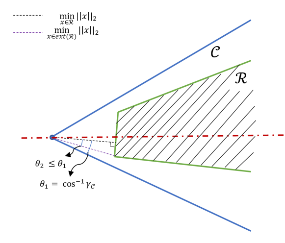
An illustration of this lemma in the case of is given in Figure 7. Note that, measures the pointedness of the cone . Geometrically (for ) the lemma states that the cosine of the angle between and is smaller than .
Proof.
We write
| (B.15) |
Replacing
| (B.16) |
we get
| (B.17) | ||||
| (B.18) |
Hence, using the definition of , we have
| (B.19) |
Note that
| (B.20) |
Therefore,
| (B.21) |
and this completes the proof. ∎
The next lemma is a consequence of Lemma B.1.
Lemma B.2.
Let , , be matrices with linearly independent rows. We have
| (B.22) |
Proof.
Consider the cone , generated by vectors , i.e,
| (B.23) |
For we have
| (B.24) |
where and
| (B.25) |
Since, , we get . Thus, for , we have . Therefore, for defined as in Lemma B.1, we have . In addition, by symmetry, for , for the cone , generated by vectors we have . Hence, using Lemma B.1 for , (the set obtained by translating by ), we get for
| (B.26) | ||||
| (B.27) |
Hence,
| (B.28) | ||||
| (B.29) |
Therefore,
| (B.30) |
Now consider where , , where is invertible. We have
| (B.31) | ||||
| (B.32) | ||||
| (B.33) | ||||
| (B.34) |
Thus, using the fact that ,
| (B.35) | ||||
| (B.36) |
Therefore,
| (B.37) |
Finally, note that the function is monotone decreasing over . Hence, for , . Therefore, we get
| (B.38) |
and this completes the proof. ∎
We continue with the following lemmas on the condition number of the matrix .
Lemma B.3.
Let , ,with having full row rank. We have
| (B.39) |
In addition, if
| (B.40) |
then
| (B.41) |
Further, if
| (B.42) |
then
| (B.43) | |||
| (B.44) |
Proof.
For the sake of simplicity, we will write , Note that using the assumptions of Lemma B.3 we have
| (B.45) | ||||
where are row-stochastic matrices and . Also, , . Therefore,
| (B.46) |
In addition, note that for a row stochastic matrix , we have
| (B.47) |
Hence, for we get
| (B.48) |
In addition,
| (B.49) |
Hence, using (B.48), (B.49), for we have
| (B.50) |
Now assume that . In this case, using (B.45) we have
| (B.51) |
Therefore,
| (B.52) |
hence,
| (B.53) |
and
| (B.54) |
where is the right inverse of matrix . Note that
| (B.55) |
By permuting the rows and columns of , without loss of generality, we can assume that . We can write
| (B.56) | ||||
| (B.57) | ||||
| (B.58) | ||||
| (B.59) | ||||
| (B.60) |
Hence, for all , since is row-stochastic,
| (B.61) |
Thus,
| (B.62) | ||||
| (B.63) |
Therefore, using (B.60),
| (B.64) |
Thus, we can write
| (B.65) |
Therefore,
| (B.66) |
Hence,
| (B.67) |
From (B.45) we have . Using , we get
| (B.68) |
Further, from (B.45) we have . Using , we get
| (B.69) |
Hence, for , we have . In addition,
| (B.70) | ||||
| (B.71) |
and this completes the proof. ∎
Lemma B.4.
Let be such that has internal radius at least , and with . If is feasible for problem (2.5) and has linearly independent rows, then we have
| (B.72) |
Proof.
Let
| (B.73) |
Note that since is feasible for problem (2.5) and
| (B.74) |
Therefore, for any , writing , , we have
| (B.75) | ||||
| (B.76) |
Since has internal radius at least , there exists , and an orthogonal matrix , , such that . Hence, for every , there exists such that
| (B.77) |
Therefore, for any unit vector in column space of , for the line segment
| (B.78) |
Thus,
| (B.79) |
where is the orthogonal projection onto the line containing . Note that using (B.76), for any we have
| (B.80) |
In other words, for any , . Therefore, using (B.78) for any in column space of , we have
| (B.81) |
This implies that
| (B.82) |
Hence, for every , there exists such that
| (B.83) |
Note that has linearly independent columns. Multiplying the previous equation by the left inverse of , we get
| (B.84) |
Let
| (B.85) | |||
| (B.86) |
where is the right singular vector corresponding to the largest singular value of . Therefore, we have
| (B.87) | |||
| (B.88) |
Thus, for
| (B.89) |
Note that
| (B.90) |
Thus,
| (B.91) |
Hence,
| (B.92) |
∎
The following lemma states an important property of the optimal solution of problem (2.5).
Lemma B.5.
If and is the optimal solution of problem (2.5), then we have
| (B.93) |
Proof.
First note that since , we have
| (B.94) |
Hence, is a feasible solution for the problem (2.5). Therefore, we have
| (B.95) |
Letting , we have
| (B.96) | ||||
| (B.97) | ||||
| (B.98) |
Using the fact that (by triangle inequality) , we have
| (B.99) | ||||
| (B.100) |
where . Note that and for , the function is increasing. Hence, since
| (B.101) |
we have
| (B.102) |
Therefore,
| (B.103) |
In addition,
| (B.104) | ||||
| (B.105) | ||||
| (B.106) | ||||
| (B.107) | ||||
| (B.108) |
Hence,
| (B.109) |
Combining equations (B.103), (B.109), and (B.95), we get
| (B.110) |
This completes the proof of lemma. ∎
Lemma B.6.
Let be such that the uniqueness assumption holds with parameter , and has internal radius at least . In particular, we have for , and an orthogonal matrix . Finally assume . Then for the optimal solution of problem (2.5), we have
| (B.111) |
where is the orthogonal projector onto (in particular, is an affine map).
Proof.
Let be such that . The uniqueness assumption implies
| (B.112) |
Note that Lemma B.5 implies
| (B.113) |
Therefore,
| (B.114) |
Hence,
| (B.115) |
In addition, for a convex set , by triangle inequality we have
| (B.116) |
Therefore, using
| (B.117) |
we have
| (B.118) |
Hence,
| (B.119) |
and
| (B.120) |
In addition, similarly to the proof of Lemma B.5, we can write
| (B.121) | ||||
| (B.122) | ||||
| (B.123) | ||||
| (B.124) | ||||
| (B.125) | ||||
| (B.126) |
Thus,
| (B.127) |
Therefore, combining (B.115), (B.119), (B.120), (B.127), we get
| (B.128) |
Now, we would like to bound the terms , . Note that using the fact that is feasible for Problem (2.5), we have
| (B.129) |
Thus,
| (B.130) |
In addition, we know that , where is a dimensional affine subspace. Therefore, and, by convexity of , we get
| (B.131) |
First consider the case in which . for all . By a perturbation argument, we can assume that the rows of are linearly independent, and hence . Consider defined by
| (B.132) | |||
| (B.133) | |||
| (B.134) |
where . Note that for every , we have . In addition, since , . Hence, for , we can write
| (B.135) |
where , , , . It is easy to check that for this we have
| (B.136) |
where is such that for ,
| (B.137) |
Further, note that since , and , we have . Hence, for ,
| (B.138) |
In addition,
| (B.139) |
Therefore, every can be written as a convex combination of the rows of . Hence,
| (B.140) |
Let , . Since , by taking , we have
| (B.141) | ||||
| (B.142) | ||||
| (B.143) |
provided that . Hence, using (B.131) for this , . Note that for , we have . Thus,
| (B.144) |
Therefore, there exists such that and
Now consider the general case in which . Let be such that is the projection of onto . Assuming that the rows of are linearly independent, . Note that since , for every point , . Thus,
| (B.145) |
Therefore, using the above argument for the case where , we can find such that and
| (B.146) | |||
| (B.147) |
Hence, for every ,
| (B.148) | ||||
where orthogonal projection onto . We next use the assumption on the internal radius of to upper bound the term . Note that since , letting , for some orthogonal matrix , , we have
| (B.149) | ||||
| (B.150) |
Now, using Cauchy-Schwarz inequality we can write
| (B.151) |
Note that,
| (B.152) | ||||
| (B.153) |
Hence, using (B.151)
| (B.154) |
In particular, for we get
| (B.155) |
Taking , the singular value decomposition of , we have . Letting , we get
| (B.156) |
Letting , this results in
| (B.157) |
In addition, note that, by the internal radius assumption, for any , . Further, since ,
| (B.158) | ||||
| (B.159) | ||||
| (B.160) | ||||
| (B.161) |
where is the projector onto the column space of . Note that,
| (B.162) | ||||
| (B.163) | ||||
| (B.164) | ||||
| (B.165) | ||||
| (B.166) |
where the last inequality follows from (B.157). This results in
| (B.167) |
Therefore, . Hence, using (B.148) we get
| (B.168) | |||
| (B.169) |
Replacing this in (B.128) completes the proof. ∎
B.3.2 Proof of Theorem 2
For simplicity, let . First note that under the assumption of Theorem 2 we have
| (B.170) |
Therefore, using Lemma B.4 with and , we have
| (B.171) |
In addition, since we have for some . Therefore,
| (B.172) |
Note that
| (B.173) |
Therefore, using Lemma B.6 we have
| (B.174) |
In addition, Lemma B.2 implies that
| (B.175) |
Further, let denote the orthogonal projector on . Hence, is a non-expansive mapping: for , . Therefore, since , for any
| (B.176) |
Therefore,
| (B.177) |
First consider the case in which
| (B.178) |
Note that in this case . Hence, using Lemma B.3 to upper bound , and Lemma B.4 to lower bound , by (B.177), we get
| (B.179) | |||
| (B.180) |
Replacing these in (B.174) we have
| (B.181) |
Therefore,
| (B.182) |
Notice that condition (B.178) implies that and
| (B.183) |
Using the previous two equations, under condition (B.178) we have
| (B.184) |
Combining this with (B.175), and using the fact that , we have under condition (B.178)
| (B.185) | ||||
| (B.186) |
Note that using (B.171), (B.172) and since
| (B.187) |
Therefore,
| (B.188) |
Thus,
| (B.189) |
where is defined in Theorem 2.
Next, consider the case in which
| (B.190) |
Note that using (B.171),(B.172) and since , this condition on implies that
| (B.191) |
In particular, condition (B.178) holds. Hence, using equation (B.184) we get
| (B.192) |
Further, note that since is a projection onto an affine subspace, for , for some . Hence, for any , , we have
| (B.193) |
where is the ’th standard unit vector. Hence,
| (B.194) |
Thus, for an arbitrary row of , we have
| (B.195) |
In addition, using non-expansivity of , we have
| (B.196) |
This implies that
| (B.197) |
Therefore, using (B.177), (B.197) and (B.192) we get
| (B.198) |
Hence, in this case Lemma B.3 implies that
| (B.199) | |||
| (B.200) |
Replacing this in (B.174), we have
| (B.201) | ||||
| (B.202) |
Hence, using (B.175) under assumption (B.190), we have
| (B.203) | ||||
| (B.204) |
Hence, for as defined in the statement of the theorem, we get
| (B.205) |
This completes the proof.
Appendix C Proof of Proposition 4.2
The proof follows immediately from the following two propositions.
Proposition C.1.
Let and . Then the gradient of the function is given by
| (C.1) |
Proof.
Note that is the solution of the following convex optimization problem.
| (C.2) | ||||
The Lagrangian for this problem is
| (C.3) |
The KKT condition implies that at the minimizer , we have
| (C.4) |
and therefore
| (C.5) |
and the dual of the above optimization problem is
| (C.6) | ||||
Note that since (C.2) is strictly feasible, Slater condition holds and by strong duality the optimal value of (C.6) is equal to . Hence, we have written as pointwise supremum of functions. Therefore, subgradient of can be achieved by taking the derivative of the objective function in (C.6) at the optimal solution (see Section 2.10 in [MN13]). Note that the derivative of this objective function at the optimal solution is equal to (where we used Eq. (C.5)). Since the dual optimum is unique (by strong convexity in ), the function is differentiable with gradient given by Eq. (C.1). ∎
Proposition C.2.
Let and , and assume that the rows of are affine independent. Then the function is differentiable at with gradient
| (C.7) |
Proof.
We will denote by the right hand side of Eq. (C.7). For , we have
| (C.8) |
Note that has affinely independent rows for in a neighborhood of , and hence has a unique minimizer there, that we will denote by . By optimality of , we have
| (C.9) | ||||
| (C.10) | ||||
| (C.11) |
On the other hand, by optimality of ,
| (C.12) | ||||
| (C.13) | ||||
| (C.14) |
Letting denote the residual, we get
| (C.15) |
Note that must converge to as because is the unique minimizer for . Hence we get as , which proves our claim. ∎
Appendix D Proof of Proposition 4.1
We use the results of [BST14] to prove Proposition 4.1. We refer the reader to [BST14] for the definitions of the technical terms in this section. First, consider the function
| (D.1) |
Note that using the main theorem of polytope theory (Theorem 1.1 in [Zie12]), we can write
| (D.2) |
for some , and a finite . Hence, using the definition of the semi-algebraic sets (see Definition 5 in [BST14]), the set is semi-algebraic. Therefore, the function which is proportional to the sum of squared distances of the rows of from a semi-algebraic set, is a semi-algebraic function (See Appendix in [BST14]). Further, the function
| (D.3) |
is the sum of indicator functions of semi-algebraic sets (Note that using the same argument used for , is semi-algebraic). Therefore, the function is semi-algebraic (See Appendix in [BST14]). In addition, the function
| (D.4) |
is a polynomial. Hence, it is semi-algebraic. Therefore, we deduce that the function
| (D.5) |
is semi-algebraic. In addition, since is closed, is proper and lower semi-continuous. Therefore, is a KL function (See Theorem 3 in [BST14]).
Now, we will show that the Assumptions 1,2 in [BST14] hold for our algorithm. First, note that since is closed, the functions and are proper and lower semi-continuous. Further, for all . In addition, the function is . Therefore, it is Lipschitz continuous over the bounded subsets of . Also, the partial derivatives of are
| (D.6) | |||
| (D.7) |
It can be seen that for any fixed , the function is Lipschitz continuous with moduli . Similarly, for any fixed , the function is Lipschitz continuous with moduli . Note that since in each iteration of the algorithm the rows of are in . Hence,
| (D.8) |
for some some positive constants . In addition, note that because the PALM algorithm is a descent algorithm, i.e., for , and since as , the value of remains bounded in every iteration. Finally, note that by taking for some constant , we make sure that the steps in the PALM algorithm remain well defined (See Remark 3(iii) in [BST14]). Hence, we have shown that the assumptions of Theorem 1 in [BST14] hold. Therefore, using this theorem, the sequence generated by the iterations in (4.7) - (4.9) has a finite length and it converges to a stationary point of .
Appendix E Other optimization algorithms
Apart from the proximal alternating linearized minimization discussed in Section 4.2, we experimented with two other algorithms, obtaining comparable results. For the sake of completeness, we describe these algorithms here.
E.1 Stochastic gradient descent
Using any of the initializations discussed in Section 4.1 we iterate
| (E.1) |
The step size is selected by backtracking line search. Ideally, the direction can be taken to be equal to . However, for large datasets this is computationally impractical, since it requires to compute the projection of each data point onto the set . In order to reduce the complexity of the direction calculation, we estimate this sum by subsampling. Namely, we draw a uniformly random set of fixed size , and compute
| (E.2) | ||||
| (E.3) |
E.2 Alternating minimization
This approach generalizes the original algorithm of [CB94]. We rewrite the objective as a function of , ,, and ,
| (E.4) | ||||
| (E.5) |
The algorithm alternates between minimizing with respect to the weights (this can be done independently across ) and minimizing over , which is done sequentially by cycling over . Minimization over can be performed by solving a non-negative least squares problem. As shown in [CB94], minimization over is also equivalent to non-negative least squares. Indeed, by a simple calculation
| (E.6) | ||||
| (E.7) |
where , does not depend on , and we defined
| (E.8) | ||||
| (E.9) |
It is therefore sufficient to minimize with respect to its first two arguments, which is equivalent to a non-negarive least squares problem. This can be seen by minimizing explicitly with respect to and writing the resulting objective function.
The pseudocode for this algorithm is given below.
| Alternating minimization | |
|---|---|
| Input : Data , ; integer ; initial archetypes ; number of iterations ; | |
| Output : Archetype estimates ; | |
| 1: | For : |
| 2: | Set ; |
| 3: | For : |
| 4: | Set |
| 5: | For : |
| 6: | Set ; |
| 7: | End For; |
| 8: | Return |
Here , , and similarly for .