Alternative transient eddy-current
flowmetering methods for liquid metals

Abstract

We present a comprehensive numerical analysis of alternative transient eddy-current flowmetering methods for liquid metals. This type of flowmeter operates by tracking eddy-current markers excited by the magnetic field pulses in the flow of a conducting liquid. Using a simple mathematical model, where the fluid flow is replaced by a translating cylinder, a number possible alternative measurement schemes are considered. The velocity of the medium can be measured by tracking zero crossing points and spatial or temporal extrema of the electromotive force (emf) induced by transient eddy currents in the surrounding space. Zero crossing points and spatial extrema of the emf travel synchronously with the medium whereas temporal extrema experience an initial time delay which depends on the conductivity and velocity of the medium. Performance of transient eddy-current flowmetering depends crucially on the symmetry of system. Eddy current asymmetry of a few per cent makes the detection point drift with a velocity corresponding to a magnetic Reynolds number $\mathit{Rm}\sim 0.1.$ With this level of asymmetry transient eddy-current flowmetering can be reliably applicable only to flows with $\mathit{Rm}\gtrsim 0.1.$ A more accurate symmetry adjustment or calibration of flowmeters may be necessary at lower velocities.

1 Introduction

Accurate and reliable flowmetering of molten metals is required not only in various metallurgical processes but also in the nuclear industry where liquid metals are used for cooling of advanced reactors [1, 2, 3]. The application of standard induction flowmeters to molten metals is limited by their chemical aggressiveness which may cause corrosion of electrodes and other contact problems. There is a variety of contactless flowmeters which have been developed to avoid the problems with electrodes. Induction flowmeters can be made contactless by using capacitately-coupled electrodes [4, 5]. However, most contactless electromagnetic flowmeters for liquid metals employ various effects related to eddy currents. For example, the flow rate can be determined by measuring the force generated by eddy currents on a magnet placed close to the flow of conducting liquid, as first suggested by Shercliff [6] and recently pursued by the so-called Lorentz Force Velocimetry [7, 8]. An alternative approach, which is virtually force-free and thus largely independent of the conductivity of liquid metal [9], is to determine the flow rate from the equilibrium rotation rate of a freely rotating magnetic flywheel [10, 11, 12, 13] or just a single magnet [14].

The standard eddy-current flowmeters operate by measuring the flow-induced perturbation of the applied magnetic field [15, 16, 17]. The same principle underlies also the so-called flow tomography which can reconstruct the basic features of the flow using the spatial distribution of the induced magnetic field [18, 19]. The application of this type of flowmeters becomes problematic when the induced magnetic field is significantly weaker than the external field, which is the case at low velocities. Although the background signal produced by the transformer effect of the applied magnetic field can be compensated by a proper arrangement of sending and receiving coils [20], standard eddy-current flowmeters remain highly susceptible to small geometrical imperfections and disturbances. The sensitivity of eddy-current flowmeters to such geometrical disturbances can significantly be reduced by measuring the phase shift induced by the flow between two sensor coils instead of the usual amplitude difference [21]. One of the remaining drawbacks of the phase-shift flowmeter is the dependence of the signal not only on the velocity but also on the conductivity of liquid metal. This is a general problem which affects not only eddy-current but also the Lorentz force flowmeters unless based on the elaborate time-of-flight measurements [22]. Recently, we showed that the sensitivity of the phase-shift flowmeter to the variations of conductivity of liquid metal can be significantly reduced by rescaling the flow-induced phase shift between the receiving coils with the phase shift between the sending and one of the receiving coils [23].

Another electromagnetic flowmeter, which is largely insensitive to the conductivity of medium, is the pulsed field flowmeter [24, 25]. This type of device, which has been recently developed under the name of transient eddy-current flowmeter [26] and claimed to be calibration free [27], operates by exciting and then tracking transient eddy current markers as they are carried along by a moving conductor.

In this paper, we present a comprehensive numerical analysis of alternative designs of transient eddy flowmeters which differ by the feature of eddy current distribution tracked. The velocity of the medium can be determined by tracking either zero crossing points or extrema of the induced emf. There are two types of extrema – spatial and temporal, which can be tracked. We point out that the transient eddy-current flowmetering relies essentially on the symmetry of the system.

The paper is organized as follows. In the next section, we introduce a mathematical model of a transient eddy-current flowmeter where the liquid flow is substituted by an infinite cylinder that translates along its axis. The basics of the method are discussed in Sec. 3 where the temporal evolution of axially mono-harmonic eddy current eigenmodes are considered. In Section 4 we present numerical results for axially mono-harmonic eddy current distributions as well as more realistic distributions generated circular current loops. The paper is concluded by a summary and discussion of results in Section 5.

2 Mathematical Model

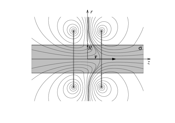
Figure 1: Sketch of set-up showing a cylinder of radius $R$ and electrical conductivity $\sigma$ translating at velocity $\bm{v}$ parallel to its axis in the magnetic field generated by two anti-symmetric current loops.

Consider a solid infinitely long cylinder of radius $R$ and electrical conductivity $\sigma$ translating at a velocity $\bm{v}=\bm{e}_{z}v$ parallel to its axis in an external magnetic field $\bm{B}_{0},$ which is periodically switched on and off for the time intervals $\tau$ and $T-\tau,$ respectively, where $T$ is the period of one full cycle. The induced electric field is governed by the Maxwell-Faraday equation

$$\bm{E}=-\bm{\nabla}\varphi-\partial_{t}\bm{A},$$

where $\varphi$ is the electric potential and $\bm{A}$ is the vector potential, which defines the magnetic field as $\bm{B}=\bm{\nabla}\times\bm{A}$. The eddy current density induced in a moving medium is given by Ohm’s law

$$\bm{j}=\sigma(\bm{E}+\bm{v}\times\bm{B})=\sigma(-\bm{\nabla}\varphi-\partial_{t}\bm{A}+\bm{v}\times\bm{\nabla}\times\bm{A}).$$ (1)

In the following, we consider an axisymmetric magnetic field which has only $r$ and $z$ components in the cylindrical system of coordinates and, thus, can be described by a purely azimuthal vector potential $\bm{A}=\bm{e}_{\phi}A$ as $\bm{B}=-r^{-1}\bm{e}_{\phi}\times\bm{\nabla}(rA)$ with $\varphi\equiv 0.$ Note that $\bm{B}\cdot\bm{\nabla}(rA)\equiv 0,$ which means that the isolines of $rA=\Phi$ represent the flux lines of $\bm{B}.$ Applying Ampere’s law $\bm{j}=\mu_{0}^{-1}\bm{\nabla}\times\bm{B}$ to Eq. (1) we obtain the following advection-diffusion equation for $A(\bm{r})$

$$\mu_{0}\sigma(\partial_{t}A+v\partial_{z}A)=\partial_{r}(r^{-1}\partial_{r}(rA))+\partial_{z}^{2}A,$$ (2)

where $\mu_{0}=4\pi\times 10^{-7}\,\mathrm{H/m}$ is the vacuum permeability. The continuity of $\bm{B}$ at the cylinder surface at $r=1$ requires the continuity of $A$ and $\partial_{r}A.$

Subsequently, we change to dimensionless variables by using $R,$ $\tau_{m}=\mu_{0}\sigma R^{2}$ and $v_{m}=(\mu_{0}\sigma R)^{-1}$ as the length, time and velocity scales, respectively. Then the problem is defined by the magnetic Reynolds number $\mathit{Rm}=\mu_{0}\sigma vR,$ which represents a dimensionless velocity.

We first consider the evolution of the eddy currents induced by the external magnetic field in the form of a single Fourier harmonic which varies as

$$A_{0}(r,z,t)=\hat{A}_{0}(r)\sin(kz)f(t),$$

where $k$ is the wave number and

$$f(t)=\left\{\begin{array}[]{ll}\eta(t)+\eta(\tau-t)-\eta(T-t),&0\leq t<T\\ f(t-T),&t>T\end{array}\right.=\sum_{n=-N/2}^{N/2}f_{n}e^{i\omega_{n}t}$$

is the time variation which is defined using the complementary error function $\eta(t)\text{=erfc}(t/\delta)$ to allow for a finite transition time $\delta$ between the “on” and “off” states. This transition time, which we set to three sampling time intervals $T/N$, is necessary to suppress the Gibbs phenomenon in the Fourier series representation of $f(t).$ The Fourier coefficients $f_{n}$ for the modes with frequencies $\omega_{n}=2\pi n/T$ are computed using the FFT with a typical number of sampling points $N=1024.$ The solution can be represented in the complex form as

$$A(r,z,t)=\sum_{n=-N/2}^{N/2}\Im\left[\hat{A}_{n}(r)f_{n}e^{i(\omega_{n}t+kx)}\right].$$

The radial distribution of the magnetic field outside the cylinder is given by the general solution of Eq. (2) with $\sigma=0$

$$\hat{A}_{n}(r)=CI_{1}(kr)+D_{n}^{o}K_{1}(kr),$$ (3)

where $I_{\nu}(x)$ and $K_{\nu}(x)$ are the modified Bessel functions of the first and second kind with order $\nu$ [28]; $C$ is an unknown constant which depends on the current distribution generating the field and $D_{n}^{o}$ is an unknown constant associated with the $n$-th harmonic of the induced magnetic field. Inside the cylinder, the solution of Eq. (2) which is regular at the axis $r=0$ is

$$\hat{A}_{n}(r)=D_{n}^{i}I_{1}(\kappa r),$$ (4)

where $\kappa=\left(k^{2}+i(\omega_{n}+k\mathit{Rm})\right)^{1/2}.$ The unknown constants $D_{n}^{o}$ and $D_{n}^{i}$ are determined by the continuity conditions of $A$ as follows

$$D_{n}^{o} = C_{n}(kI_{0}(k)I_{1}(\kappa)-\kappa I_{0}(\kappa)I_{1}(k)),$$

$$D_{n}^{i} = C_{n}k(K_{0}(k)I_{1}(k)+I_{0}(k)K_{1}(k)),$$

where $C_{n}=C/(kK_{0}(k)I_{1}(\kappa)+\kappa I_{0}(\kappa)K_{1}(k)).$ Since the current amplitude is irrelevant in our analysis, we can set $C=1.$

The solution for a single Fourier harmonic obtained above can be extended to a more realistic external magnetic field generated by a thin circular loop. The free-space distribution of the magnetic field, which is generated by a single current loop with radius $r_{c}$ and axial position $z_{c}$ carrying the dimensionless current $j_{c}$, is governed by

$$\bm{\nabla}^{2}A_{0}=-j_{c}\delta(\bm{r}-r_{c}\bm{e}_{r}-z_{c}\bm{e}_{z}),$$ (5)

where $\delta(\bm{r})$ is the Dirac delta function and $\bm{r}$ is the radius vector. This problem can easily be solved using the Fourier transform $\hat{A}(r)=\int_{-\infty}^{\infty}A(r,z)e^{ikz}\,dz,$ which converts Eq. (5) into

$$(r^{-1}(r\hat{A}_{0})^{\prime})^{\prime}-k^{2}\hat{A_{0}}=-\hat{j}_{c}\delta(r-r_{c}),$$ (6)

where $\hat{j}_{c}=j_{c}e^{-ikz_{c}}.$ The solution, which is continuous at $r=r_{c}$, regular at $r=0,$ and decays at $r\rightarrow\infty,$ can be written as

$$\hat{A}_{0}(r)=\left\{\begin{array}[]{ll}D_{c}I_{1}(kr)/I_{1}(kr_{c}),&r<r_{c};\\ D_{c}K_{1}(kr)/K_{1}(kr_{c}),&r>r_{c},\end{array}\right.$$

where $D_{c}=-\hat{j}_{c}/k\left(I_{0}(kr_{c})/I_{1}(kr_{c})+K_{0}(kr_{c})/K_{1}(kr_{c})\right)$ follows from the integration of Eq. (6) over the singularity at $r=r_{c}.$ Then the unknown constant defining the distribution of the applied magnetic field in Eq. (3) can be written as $C=\sum_{c}D_{c}/I_{1}(kr_{c})$ where the summation is over the current loops generating the field. The vector potential in physical space is obtained by the inverse Fourier transform which is computed using the FFT with a typical number of sampling points $M=1024$ and axial cut-off distance $z_{\max}=\pm 51.2.$

3 Eigenmode evolution

The basics of transient eddy-current flowmetering are best revealed by the evolution of separate eigenmodes, which can be sought in the complex form as

$$A(r,z,t)=\hat{A}(r)e^{ikz-\gamma t},$$ (7)

where $k$ is a given real wave number and $\gamma$ is an unknown complex decay rate. The latter has to be determined together with the amplitude distribution $\hat{A}(r)$ by solving the eigenvalue problem posed by Eq. (2). In the absence of external magnetic field, the solution outside the cylinder (3) reduces to

$$\hat{A}(r)=D^{o}K_{1}(kr),$$ (8)

where $D^{o}$ is an unknown constant. Inside the cylinder, the general solution of Eq. (2) can be written as

$$\hat{A}(r)=D^{i}J_{1}(\alpha r),$$

where $D^{i}$ is another unknown constant, $J_{\nu}(x)$ is the Bessel function of the first kind and order $\nu,$ and $\alpha=\left(\gamma-k^{2}-ik\mathit{Rm}\right)^{1/2}.$ The continuity of $A$ and its first derivative leads to the following characteristic equation

$$\alpha J_{0}(\alpha)/K_{0}(k)+kJ_{1}(\alpha)/K_{1}(k)=0,$$ (9)

which has real roots $\alpha$ that define the complex associated decay rates

$$\gamma=\alpha^{2}+k^{2}+ik\mathit{Rm}.$$ (10)

The most important result that follows from this expression is the constant phase speed $\Im[\gamma]/k=\mathit{Rm}$ at which all eddy current patterns travel regardless of their wave number. Note that the corresponding physical velocity $\mathit{Rm}v_{m}=v$ is that of the medium. This means that the velocity of the medium can be determined by measuring the phase velocity at which an eddy current pattern is advected. This is the main idea behind the transient eddy-current flowmetering.

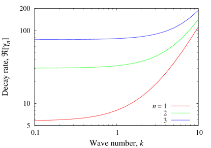
Figure 2: Three lowest eddy current decay rates versus the wave number.

The second important result that follows from Eqs. (9,10) concerns the decay rate $\Re[\gamma]$. As seen in figure 2, where the decay rates of the first three dominant eigenmodes are plotted against the wave number, the lowest decay rates occur in the long wave limit $k\rightarrow 0.$ In this limit, the characteristic equation (9) reduces to $J_{0}(\kappa)=0$ and yields $\Re[\gamma_{1}]\approx 5.78.$ It means that the eddy current amplitude drops by almost three orders of magnitude over the the characteristic magnetic diffusion time $\tau_{m}=\mu_{0}\sigma R^{2}.$ The decay times of subsequent eigenmodes are significantly shorter. It implies that the time interval over which a transient eddy current pattern can be tracked is limited by a few magnetic diffusion time scales $t_{m}.$ The respective dimensionless distance over which the pattern is advected is, thus, limited by a few $\mathit{Rm}.$

The decay of eddy currents makes the determination of their phase speed more complicated than for a constant-amplitude wave. For the latter, the phase velocity describes the motion of points with a fixed amplitude. In a decaying wave, the only points whose amplitude remains constant in time are those at which the oscillating quantity passes through zero. Depending on the physical quantity whose zero crossing is tracked, several alternatives of transient eddy-current flowmetering are possible. Mathematically, the alternative quantities are related with temporal or spatial derivatives of eddy current distribution. For example, the emf induced by a decaying eddy current, which gives rise to voltage in the pick-up coils, is related with the time derivative of the associated magnetic flux. In our case, the latter is defined by $\mathcal{E}=-\partial_{t}\Phi.$ Instead of zero crossings one can also track extrema of $\mathcal{E}$, either in space or time, which are defined mathematically by the zero crossings of $\partial_{z}\mathcal{E}$ and $\partial_{t}\mathcal{E},$ respectively.

4 Results

4.1 Mono-harmonic eddy current distribution

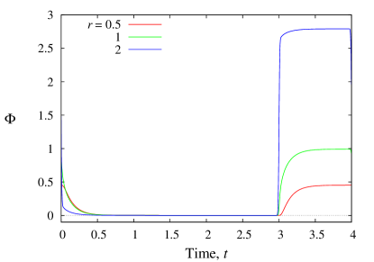
Figure 3: Variation of the magnetic flux $\Phi=rA$ over one time period at $z=0.5$ and $r=0.5,\,1,\,2$ for the Fourier harmonic with the wave number $k=1$ when the cylinder is at rest $(\mathit{Rm}=0)$ (a); variation of the emf magnitude $|\partial_{t}\Phi|$ with time at the same points for $\mathit{Rm}=0$ and $\mathit{Rm}=1$ (b).

Let us start with an external magnetic field which is periodically switched off and on for the dimensionless time intervals $\tau=3$ and $T-\tau=1,$ respectively. According to the previous eigenvalue analysis, these time intervals are sufficiently long for the eddy currents to develop. This is confirmed by the temporal variation of the magnetic flux $\Phi=rA$ shown in Fig. 3(a) for the wave number $k=1$ at $z=0.5$ and three different radii when the cylinder is at rest $(\mathit{Rm}=0).$ The respective variation of the emf magnitude is plotted in Fig. 3(b). When the cylinder is at rest $(\mathit{Rm}=0),$ the emf is seen to decrease exponentially with time as predicted by the previous eigenvalue analysis. When the cylinder moves with velocity $\mathit{Rm}=1$ the decrease of emf is accompanied by a zero crossing, which for the observation point located at $z=0.5$ occurs at the time instant $t\approx 0.5.$ This point is seen as the cusp on the semi-logarithmic plot of $|\mathcal{E}|$ in Fig. 3(b). Shortly after passing through zero, emf is seen to attain a local extremum, which is defined mathematically by zero crossing of $\partial_{t}\mathcal{E}.$

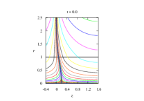
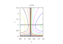
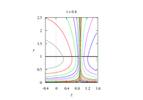
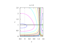
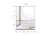
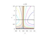
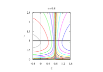
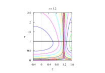
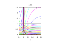
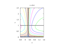
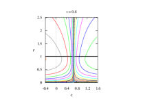
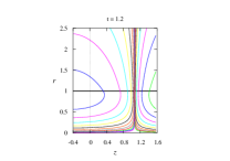
Figure 4: The magnetic flux lines $(\Phi=\text{const)}$ (top), the isolines of emf $\mathcal{E}=-\partial_{t}\Phi$ (middle), and of $\partial_{t}\mathcal{E}=-\partial_{tt}^{2}\Phi$ (bottom) for $\mathit{Rm}=1$ at the time instants $t=0,\,0.4,\,0.8,\,1.2$ after a mono-harmonic external magnetic field with the wave number $k=1$ has been switched off. Subsequent isolevels differ by a factor of two and cluster around zero value.

Figure 4 shows the evolution of the magnetic field pattern and the associated emf with wave number $k=1$ after switching external magnetic field off for the cylinder moving with velocity $\mathit{Rm}=1.$ It may be seen that the zero crossing of the emf, which is marked by the increased density of isolines in the middle row, closely follows the medium by being located at $z=t\mathit{Rm}.$ Thus, the velocity of medium can be determined directly as $\mathit{Rm}=z/t,$ where $z$ is the axial distance of the observation point from the wave node and $t$ is the time at which the emf passes through zero at that point after switching the field off. The pattern of the magnetic flux lines, which is shown at the top row of Fig. 4, may be seen to run slightly ahead of that of the emf. This is obviously due to the effect of advection, which tilts the magnetic flux lines in the direction of motion. On the other hand, the time derivative, which is equivalent to the multiplication of the dominating eigenmode (7) by $-\gamma,$ causes a phase shift of the resulting distribution by $\arg(-\gamma).$ Thus, the pattern of $\partial_{t}\mathcal{E}$, which is shown in the bottom row of Fig. 4, lags slightly behind that of $\mathcal{E}.$ Note that the zero crossing of $\partial_{t}\mathcal{E},$ which like that of $\mathcal{E}$ is marked by the increased density of the isolines, indicates the location of temporal extremum of $\mathcal{E}.$ Location of spatial extremum of $\mathcal{E}$ is defined by zero crossings of $\partial_{z}\mathcal{E}.$ For a mono-harmonic eddy current, the distribution of $\partial_{z}\mathcal{E}=ik\mathcal{E}$ is shifted by a quarter wave length relative to that of $\mathcal{E}.$ Therefore the spatial extrema of emf in a mono-harmonic wave move in exactly the same way as zero crossings.

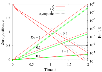
Figure 5: (a) Axial zero crossing positions of $\mathcal{E}$ and $\partial_{t}\mathcal{E}$ as well as the relative magnitude of $\mathcal{E}$ against time for mono-harmonic eddy current distributions with $k=0.5,\,1$ and $\mathit{Rm}=0.1,\,0.5,\,1.$ (b) Axial zero crossing positions of $\mathcal{E},\partial_{t}\mathcal{E}$ and $\partial_{z}\mathcal{E},\partial_{z}\Phi$ for the eddy current distributions generated respectively by two antisymmetric and a single current loop with the radius $r=2$ and placed at $z=\pm 1$ and $z=0.$

As zero crossing outside the cylinder is seen in Fig. 4 to occur synchronously along the radius, in the following we focus on the emf distribution along the surface $r=1.$ Figure 5(b) shows zero crossing positions of both $\mathcal{E}$ and $\partial_{t}\mathcal{E}$ against time as well as the respective evolution of the emf amplitude for two mono-harmonic eddy current distributions with wave numbers $k=1$ and $k=0.5$ and three different velocities $\mathit{Rm}=0.1,\,0.5,\,1.$ Firstly, the emf for both distributions may be seen to decay in a good agreement with the analytically determined damping rates for the respective wave numbers. Secondly, the zero crossing points of $\mathcal{E}$ in both waves move in exactly the same way with velocity $\mathit{Rm}$ starting from the node $z=0$. Temporal extrema points, which correspond to zero crossings of $\partial_{t}\mathcal{E},$ also move at the same velocity as the medium but with a time delay which depends on the wave number $k$ as well as on the velocity $\mathit{Rm}$ itself. It means that at least two measurement points are required to eliminate this offset and, thus, to determine the velocity of the medium using temporal extrema of emf.

4.2 Eddy currents induced by circular loops

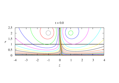
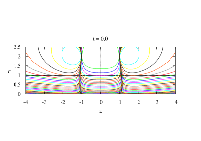
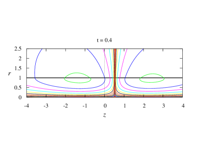
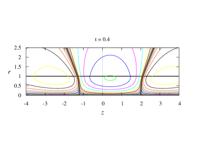
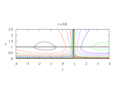
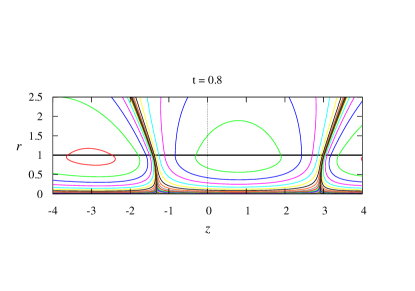
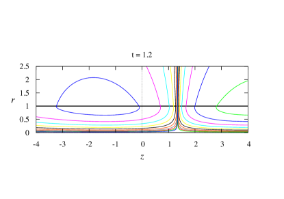
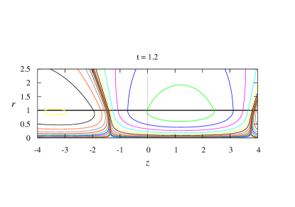
Figure 6: The magnetic flux lines $(\Phi=\text{const)}$ (left) and the isolines of $\partial_{z}\mathcal{E}=-\partial_{tz}^{2}\Phi$ (right) at the time instants $t=0,\,0.4,\,0.8,\,1.2$ after the external magnetic field generated by a pair of antisymmetric current loops with radius $r_{c}=2$ located at $z_{c}=\pm 1$ has been switched off.

Now let us consider the evolution of eddy currents generated by realistic coils made of circular loops. We start with an antisymmetric coil configuration consisting of two circular loops of radius $r_{c}=2$ which are placed at $z_{c}=\pm 1$ and carry equal but opposite currents. This configuration creates a zero crossing of emf at the symmetry plane $z=0$ between the loops which is analogous to the wave node of the mono-harmonic distribution considered in the previous section. As a result, the advection of the field pattern by the moving medium, which is shown for $\mathit{Rm}=1$ in Fig. 6(left), is similar to that of the mono-harmonic eddy current distribution in Fig. 4(top). Also the zero crossing points of $\mathcal{E}$ and $\partial_{t}\mathcal{E}$ move in the same way as in the mono-harmonic wave. But there is one substantial difference between the mono-harmonic and anti-symmetric eddy-current distributions which concerns the motion of spatial extrema of emf. There are two such extrema, which are seen in Fig. 6(right) to be located at the current loops where zero crossings of $\partial_{z}\mathcal{E}$ are marked by the increased density of isolines. First of all, it is obvious that these extrema do not move at the same velocity. Namely, the right (downstream) extremum moves noticeably faster than the medium whereas the left (upstream) one moves not only much slower but also in the opposite direction. The main difference between the spatial extrema in the previous mono-harmonic and the present two-loop eddy current distributions is the absence of symmetry in the latter. It will be shown later that symmetry is crucial to the transient eddy current flowmetering.

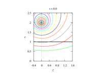
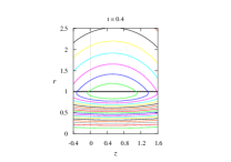
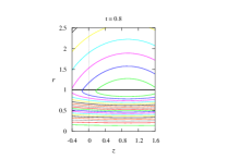
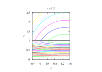
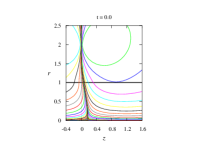
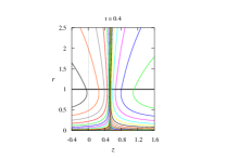
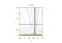
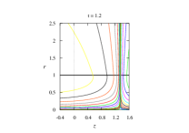
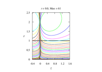
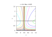
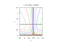
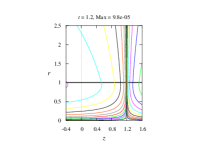
Figure 7: The magnetic flux lines $(\Phi=\text{const)}$ (top), the isolines of $\partial_{z}\Phi$ (middle) and $\partial_{z}\mathcal{E}=-\partial_{zt}^{2}\Phi$ (bottom) for $\mathit{Rm}=1$ at the time instants $t=0,\,0.4,\,0.8,\,1.2$ after the external magnetic field generated by a single current loop located at $r_{c}=2$ and $z_{c}=0$ has been switched off. Levels of subsequent isolines differ by a factor of two and the increased density of isolines indicates zero value.

Eddy current distribution with a spatially symmetric emf extremum but without zero crossing can be generated using a single current loop [25]. The evolution of the field pattern generated by a current loop of radius $r_{c}=2$ placed at $z_{c}=0$ is shown in Fig. 7 for $\mathit{Rm}=1.$ In this case, there are neither zero crossings nor temporal extrema of emf but only axial extrema of the magnetic flux and emf. These extrema, which are respectively located at the zero crossings of $\partial_{z}\Phi=-rB_{r}$ and $\partial_{z}\mathcal{E},$ move synchronously with the medium. The axial extremum of emf is seen to move without the time lag as the zero crossing in the anti-symmetric set-up, whereas the flux extremum experiences a time lag similar to that of the temporal emf maximum in the anti-symmetric set-up. Note that the axial extremum of the magnetic flux can be detected as a zero crossing of the radial flux component $B_{r}$ using, for example, a Hall sensor. Also note that at least two sensor coils are required to detect an axial maximum of emf, whereas one coil can be used to detect zero crossing or temporal extremum of emf in the antisymmetric set-up. The latter, however, requires two excitation coils.

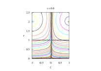
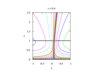
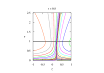
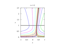
Figure 8: The emf isolines for $\mathit{Rm}=0$ at the time instants $t=0,\,0.4,\,0.8,\,1.2$ after the external magnetic field generated by a pair of opposite current loops located at $r_{c}=2$ and $z_{c}=\pm 1$ with the current asymmetry of $S=5\%$ has been switched off.

Finally, let us examine the effect of a possible asymmetry in the initial eddy current distribution generated by a two-coil set-up with opposite but slightly different currents. To characterize this kind of asymmetry we use the parameter $S=(j_{+}-j_{-})/(j_{+}+j_{-}),$ where $j_{+}$ and $j_{-}$ are the currents in the coils placed respectively on the left and right from $z=0.$ Temporal evolution of eddy current distribution with the initial asymmetry of $S=5\%$ generated by two coils of radius $r_{c}=2$ placed $z_{c}=\pm 1$ is shown in Fig. 8 for the medium at rest $(\mathit{Rm}=0).$ Because for $S>0$ the current in the coil on the left is higher than that on the right the initial emf pattern at $t=0$ is slightly tilted to the right. In contrast to the perfectly anti-symmetric distribution, where each Fourier mode of emf crosses zero at $z_{c}=0$ independently of other harmonics, in the asymmetric distribution, the zero crossing is a result of superposition of different Fourier modes. Because different harmonics decay at different rates depending on their wave number, the zero crossing line in the asymmetric distribution is not stationary but drifts to the right, as seen in Fig. 8. The direction of this drift is reversed for negative $S.$ As seen in Fig. 9, after a relatively short initial transient time, the drift velocity slightly increases and then saturates at the level which rises with the asymmetry $S$ and is nearly the same for zero crossing and temporal extremum of emf. The drift velocity averaged over the time interval from $t=0$ to $t=3$ is seen in Fig. 9 to increase nearly linearly with $S.$ At the same time the drift velocity reduces with the increase of axial separation between the coils whereas their radius has a relatively weak effect.

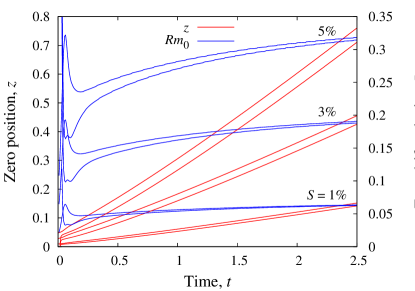
Figure 9: (a) Axial position of zero crossing and its drift velocity along the surface of cylinder at rest $(\mathit{Rm}=0)$ against the time after the external magnetic field generated by a pair of opposite current loops located at $r_{c}=2$ and $z_{c}=\pm 1$ with the current asymmetry $S$ has been switched off. The upper and lower curves correspond to the zero crossing of emf $($$\mathcal{E}=-\partial_{t}\Phi)$ and its temporal derivative $($$\partial_{t}\mathcal{E})$, respectively. (b) Zero drift velocity depending on the current asymmetry $s$ in two circular loops with radii $r_{c}=1.5,\,2,\,2.5$ placed at the axial positions $\pm z_{c}=0.5,\,0.75,\,1,\,1.5,\,2.$

5 Summary and conclusions

We have carried out a comprehensive numerical analysis of a transient eddy-current flowmetering method which is applicable to liquid metals. The method works by exciting and then tracking eddy currents as they are advected by a moving conductor. Because eddy currents decay by about three orders of magnitude over the characteristic characteristic magnetic diffusion time $\tau_{m}=\mu_{0}\sigma R^{2},$ which is $\sim 0.1\,\mathrm{s}$ in a liquid metal with a characteristic conductivity $\sigma\sim 10^{6}\,\mathrm{S/m}$ and size $R\sim 0.1\,\mathrm{m,}$ the time interval over which they can be tracked is limited to a few magnetic diffusion time scales $\tau_{m}.$ The distance over which the eddy current pattern can be tracked scales as $\sim\mathit{Rm}.$ This means that for small $\mathit{Rm},$ the pick-up coils have to be placed sufficiently close to the excitation coils at the distance $\sim\mathit{Rm}$.

We considered several alternative measurement schemes in which different characteristic features of eddy current distributions are tracked. The trackable features are zero crossing points or extrema of the emf induced by the transient eddy currents. There are two kinds of extrema which can be tracked: temporal and spacial. The former corresponds to emf $(\mathcal{E})$ passing through extremum in time at a fixed axial position. The latter corresponds to emf passing through extremum at some axial position at a fixed instant of time. Mathematically, these two types of extrema are defined as zero crossings of $\partial_{t}\mathcal{E}$ and $\partial_{z}\mathcal{E},$ respectively. Physically, temporal extremum can be detected using a single pick-up coil, whereas at least two coils are required to detect the passage of spatial extremum.

A zero crossing point is detected by the the original measurement scheme of Zheigur and Sermons [24] using a single pick-up coil and its distance from the excitation coil to determine the flow rate. The location of excitation coil is not required by the measurement schemes of Forbriger and Stefani [26] and Krauter and Stefani [27] who use respectively three and two non-coaxial pick-up coils to track approximately the emf zero crossing point. The measurement scheme analysed numerically by Tarabad and Baker [25] is based on the detection of temporal emf extremum using a single excitation coil and two symmetric pick-up coils in the differential connection.

In the mono-harmonic eddy current distributions, which were analyzed first, the spatial extrema of emf move in the same way as zero crossings because both remain separated by a quarter wave length. In this case, the velocity of medium can be determined simply as $v=z/t,$ where $t$ is the time after the eddy current excitation at which $\mathcal{E}$ or $\partial_{z}\mathcal{E}$ passes through zero at the distance $z$ from the wave node or its extremum, respectively. Flowmetering using temporal extrema of emf is slightly more complicated because these extrema occur some time after zero crossing. This additional time delay, which shows up also in the numerical results of Tarabad and Baker [25] and significantly disturbs their measurement scheme, depends on the conductivity of medium as well as on the eddy current distribution but not on the position of the observation point provided that it is not too close to the initial zero crossing point. Therefore the additional time delay can be eliminated by using two pick-up coils placed at $z_{1}$ and $z_{2}.$ Then the velocity of the medium can be found as $v=(z_{2}-z_{1})/(t_{2}-t_{1}),$ where $t_{1}$ and $t_{2}$ are the times at which temporal extrema are detected in the respective coil. The same approach can be used to eliminate the uncertainty in the emf zero crossing time caused by the inaccuracy in the position of excitation coils. Note that the measurement scheme of Krauter and Stefani [27] is somewhat different because it relies on the assumption that the emf varies linearly in the space between the two pick-up coils. Forbriger and Stefani [26] make a similar assumption about the spatial variation of the magnetic flux density. These assumptions, which may hold for sufficiently closely spaced pick-up coils but not in general, are not required in the measurement schemes considered in this study.

We considered also more realistic eddy current distributions generated by two anti-symmetric circular current loops or a single loop. In the anti-symmetric set-up, the zero crossing point of emf as well as the subsequent temporal extremum was found to travel synchronously with the medium in the same way as with the mono-harmonic wave considered before. But this was not the case for the two spatial extrema which appear at both current loops in this set-up. These two extrema were found to move at substantially different velocities from that of the medium. This result highlights the crucial importance of symmetry which holds for zero crossing points of emf but not for the two spatial extrema in the anti-symmetric set-up. In a single-loop set-up, which generates a spatially symmetric eddy current distribution, the spatial extremum of emf was found to travel synchronously with the medium as in the mono-harmonic wave. In this set-up, the velocity of the medium can be determined by also tracking axial extremum of the magnetic flux, which coincides with the zero crossing of the radial component of the magnetic field. It has to be noted that because of the initial tilt of the magnetic flux lines in the direction motion, the extremum of magnetic flux arrives at a given observation point ahead that of emf. This time lead can be eliminated similarly to the delay of temporal extremum of emf by using two sensors as discussed above.

Finally, we analyzed the effect of a possible current asymmetry in the two-loop set-up, and showed that it gives rise to a spurious drift of the emf zero crossing point. It means that the mutual symmetry of exiting coils is crucial for the transient-eddy flowmetering. Asymmetry of a few per cent was found to result in the zero drift with a dimensionless velocity $\mathit{Rm}\sim 0.1.$ For the characteristic parameters used at the beginning of this section, the respective physical velocity is $v\sim 0.1\,\mathrm{m/s.}$ It means that with this level of asymmetry, which is not unlikely in practice, transient eddy current flowmetering can be reliable only for the flows with $\mathit{Rm}\gtrsim 0.1.$ This estimate is consistent with the lowest $\mathit{Rm}\approx 0.35$ and $\mathit{Rm}\approx 0.11$ achieved respectively by Zheigur and Sermons [24] and Forbriger and Stefani [26]. At lower velocities, a more accurate symmetry adjustment or calibration of the device may be required. This obviously applies not only to the axisymmetric systems considered in our study but also to more complex non-coaxial coil arrengements used in the previous experimental studies.

The results of this study may be useful for designing more accurate and reliable transient eddy-current flowmeters for liquid metals.

References

References

- Schulenberg and Stieglitz [2010] T. Schulenberg, R. Stieglitz, Flow measurement techniques in heavy liquid metals, Nucl. Eng. Des. 240 (9) (2010) 2077–2087.
- Eckert et al. [2011] S. Eckert, D. Buchenau, G. Gerbeth, F. Stefani, F.-P. Weiss, Some recent developments in the field of measuring techniques and instrumentation for liquid metal flows, J. Nucl. Sci. Technol. 48 (4) (2011) 490–498.
- Poornapushpakala et al. [2014] S. Poornapushpakala, C. Gomathy, J. Sylvia, B. Babu, Design, development and performance testing of fast response electronics for eddy current flowmeter in monitoring sodium flow, Flow Meas. Instrum. 38 (2014) 98–107.
- Hussain and Baker [1985] Y. Hussain, R. Baker, Optimised noncontact electromagnetic flowmeter, J. Phys. E: Sci. Instrum. 18 (3) (1985) 210.
- McHale et al. [1985] E. J. McHale, Y. Hussain, M. Sanderson, J. Hemp, Capacitively-coupled magnetic flowmeter, US Patent 4,513,624, 1985.
- Shercliff [1987] J. Shercliff, The Theory of Electromagnetic Flow-Measurement, Cambridge Science Classics, Cambridge University Press, ISBN 9780521335546, 1987.
- Thess et al. [2007] A. Thess, E. Votyakov, B. Knaepen, O. Zikanov, Theory of the Lorentz force flowmeter, New J. Phys. 9 (8) (2007) 299.
- Wegfrass et al. [2012] A. Wegfrass, C. Diethold, M. Werner, T. Fröhlich, B. Halbedel, F. Hilbrunner, C. Resagk, A. Thess, A universal noncontact flowmeter for liquids, Appl Phys Lett 100 (19) (2012) 194103.
- Priede et al. [2009] J. Priede, D. Buchenau, G. Gerbeth, Force-free and contactless sensor for electromagnetic flowrate measurements, Magnetohydrodynamics 45 (3) (2009) 451–458.
- Shercliff [1960] J. Shercliff, Improvements in or relating to electromagnetic flowmeters, GB Patent 831226, 1960.
- Bucenieks [2005] I. Bucenieks, Modelling of rotary inductive electromagnetic flowmeter for liquid metals flow control, in: Proc. 8th Int. Symp. on Magnetic Suspension Technology, Dresden, Germany, 26–28 September, 204–8, 2005.
- Buchenau et al. [2014] D. Buchenau, V. Galindo, S. Eckert, The magnetic flywheel flow meter: Theoretical and experimental contributions, Appl. Phys. Lett. 104 (22) (2014) 223504.
- Hvasta et al. [2018] M. Hvasta, D. Dudt, A. Fisher, E. Kolemen, Calibrationless rotating Lorentz-force flowmeters for low flow rate applications, Meas. Sci. Technol. 29 (7) (2018) 075303.
- Priede et al. [2011a] J. Priede, D. Buchenau, G. Gerbeth, Single-magnet rotary flowmeter for liquid metals, J. Appl. Phys. 110 (3) (2011a) 034512.
- Lehde and Lang [1948] H. Lehde, W. Lang, Device for measuring rate of fluid flow, US Patent 2,435,043, 1948.
- Cowley [1965] M. Cowley, Flowmetering by a motion-induced magnetic field, J. Sci. Instrum. 42 (6) (1965) 406.
- Poornapushpakala et al. [2010] S. Poornapushpakala, C. Gomathy, J. Sylvia, B. Krishnakumar, P. Kalyanasundaram, An analysis on eddy current flowmeter–a review, in: Recent Advances in Space Technology Services and Climate Change (RSTSCC), 2010, IEEE, 185–188, 2010.
- Stefani et al. [2004] F. Stefani, T. Gundrum, G. Gerbeth, Contactless inductive flow tomography, Phys. Rev. E 70 (5) (2004) 056306.
- Stefani and Gerbeth [2000] F. Stefani, G. Gerbeth, A contactless method for velocity reconstruction in electrically conducting fluids, Meas. Sci. Technol. 11 (6) (2000) 758.
- Feng et al. [1975] C. Feng, W. Deeds, C. Dodd, Analysis of eddy-current flowmeters, J Appl Phys 46 (7) (1975) 2935–2940.
- Priede et al. [2011b] J. Priede, D. Buchenau, G. Gerbeth, Contactless electromagnetic phase-shift flowmeter for liquid metals, Meas. Sci. Technol. 22 (5) (2011b) 055402.
- Viré et al. [2010] A. Viré, B. Knaepen, A. Thess, Lorentz force velocimetry based on time-of-flight measurements, Phys Fluids 22 (12) (2010) 125101.
- Looney and Priede [2018] R. Looney, J. Priede, Concept of a next-generation electromagnetic phase-shift flowmeter for liquid metals, (submitted to Flow Meas. Instrum.) .
- Zheigur and Sermons [1965] B. D. Zheigur, G. Y. Sermons, Pulse method of measuring the rate of flow of a conducting fluid, Magnetohydrodynamics 1 (1) (1965) 101–104.
- Tarabad and Baker [1983] M. Tarabad, R. C. Baker, Computation of pulsed field electromagnetic flowmeter response to profile change, J. Phys. D: Appl. Phys. 16 (11) (1983) 2103.
- Forbriger and Stefani [2015] J. Forbriger, F. Stefani, Transient eddy current flow metering, Meas. Sci. Technol. 26 (10) (2015) 105303.
- Krauter and Stefani [2017] N. Krauter, F. Stefani, Immersed transient eddy current flow metering: a calibration-free velocity measurement technique for liquid metals, Meas. Sci. Technol. 28 (10) (2017) 105301.
- Abramowitz and Stegun [1972] M. Abramowitz, I. A. Stegun, Handbook of Mathematical Functions, Dover, New York, 1972.