Formalising openCypher Graph Queries
in Relational Algebra

Abstract

Graph database systems are increasingly adapted for storing and processing heterogeneous network-like datasets. However, due to the novelty of such systems, no standard data model or query language has yet emerged. Consequently, migrating datasets or applications even between related technologies often requires a large amount of manual work or ad-hoc solutions, thus subjecting the users to the possibility of vendor lock-in. To avoid this threat, vendors are working on supporting existing standard languages (e.g. SQL) or standardising languages.

In this paper, we present a formal specification for openCypher, a high-level declarative graph query language with an ongoing standardisation effort. We introduce relational graph algebra, which extends relational operators by adapting graph-specific operators and define a mapping from core openCypher constructs to this algebra. We propose an algorithm that allows systematic compilation of openCypher queries.

The final publication is available at Springer via
https://doi.org/10.1007/978-3-319-66917-5_13.

1 Introduction

Context.

Graphs are a well-known formalism, widely used for describing and analysing systems. Graphs provide an intuitive formalism for modelling many real-world scenarios, as the human mind tends to interpret the world in terms of objects (vertices) and their respective relationships to one another (edges) [CollectivelyGeneratedModel].

The property graph data model [DBLP:books/igi/Sakr11/RodriguezN11] extends graphs by adding labels/types and properties for vertices and edges. This gives a rich set of features for users to model their specific domain in a natural way. Graph databases are able to store property graphs and query their contents with complex graph patterns, which otherwise would be are cumbersome to define and/or inefficient to evaluate on traditional relational databases [TrainBenchmarkSOSYM].

Neo4j, a popular NoSQL property graph database, offers the Cypher query language to specify graph patterns. Cypher is a high-level declarative query language which allows the query engine to use sophisticated optimisation techniques. Neo Technology, the company behind Neo4j initiated the openCypher project [openCypher], which aims to deliver an open specification of Cypher.

Problem and objectives.

The openCypher project provides a formal specification of the grammar of the query language and a set of acceptance tests that define the semantics of various language constructs. This allows other parties to develop their own openCypher-compatible query engine. However, there is no mathematical formalisation for the language. In ambiguous cases, developers are advised to consult Neo4j’s Cypher documentation or to experiment with Neo4j’s Cypher query engine and follow its behaviour. Our goal is to provide a formal specification for the core features of openCypher.

Contributions.

In this paper, we use a formal definition of the property graph data model [DBLP:conf/edbt/HolschG16] and relational graph algebra, which operates on multisets (bags) [DBLP:books/daglib/0020812] and is extended with additional graph-specific operators. Using these foundations, we construct a concise formal specification for the core features in the openCypher grammar. This specification is detailed enough to serve as a basis for an openCypher compiler [openCypherReport].

2 Data Model and Running Example

Data model.

A property graph is defined as $G=(V,E,\mathit{st},L,T,\mathcal{L},\mathcal{T},P_{v},P_{e})$, where $V$ is a set of vertices, $E$ is a set of edges and $\mathit{st}:E\rightarrow V\times V$ assigns the source and target vertices to edges. Vertices are labelled and edges are typed:

• $L$ is a set of vertex labels, $\mathcal{L}:V\rightarrow 2^{L}$ assigns a set of labels to each vertex.

• $T$ is a set of edge types, $\mathcal{T}:E\rightarrow T$ assigns a single type to each edge.

To define properties, let $D=\cup_{i}D_{i}$ be the union of atomic domains $D_{i}$ and let $\varepsilon$ represent the NULL value.

• $P_{v}$ is a set of vertex properties. A vertex property $p_{i}\in P_{v}$ is a partial function $p_{i}:V\rightarrow D_{i}\cup\{\varepsilon\}$, which assigns a property value from a domain $D_{i}\in D$ to a vertex $v\in V$, if $v$ has property $p_{i}$, otherwise $p_{i}(v)$ returns $\varepsilon$.

• $P_{e}$ is a set of edge properties. An edge property $p_{j}\in P_{e}$ is a partial function $p_{j}:E\rightarrow D_{j}\cup\{\varepsilon\}$, which assigns a property value from a domain $D_{j}\in D$ to an edge $e\in E$, if $e$ has property $p_{j}$, otherwise $p_{j}(e)$ returns $\varepsilon$.

In the context of this paper, we define a relation as a bag (multiset) of tuples: a tuple can occur more than once in a relation [DBLP:books/daglib/0020812]. Given a property graph $G$, relation $r$ is a graph relation if the following holds:

$$\forall A\in\mathrm{sch}(\mathit{r}):\mathrm{dom}(A)\subseteq V\cup E\cup D,$$

where the schema of $r$, $\mathrm{sch}(\mathit{r})$, is a list containing the attribute names, $\mathrm{dom}(A)$ is the domain of attribute $A$, $V$ is the vertices of $G$, and $E$ is the edges of $G$.

Property access.

When defining relational algebra expression on graph relations, it is often required (e.g. in projection and selection operators) to access a certain property of a vertex/edge. Following the notation of [DBLP:conf/edbt/HolschG16], if $x$ is an attribute of a graph relation, we use $x.p$ to access the corresponding value of property $p$. Also, $\mathcal{L}(v)$ returns the labels of vertex $v$ and $\mathcal{T}(e)$ returns the type of edge $e$.

Running example.

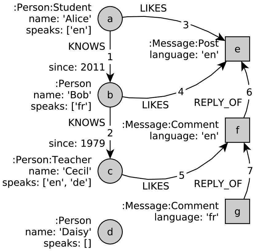
An example graph inspired by the LDBC Social Network Benchmark [DBLP:conf/sigmod/ErlingALCGPPB15] is shown on 1(a), while 1(b) presents the formalised graph. The graph vertices model four Persons and three Messages, with edges representing LIKES, REPLY_OF and KNOWS relations. In social networks, the KNOWS relation is symmetric, however, the property graph data model does not allow undirected edges. Hence, we use directed edges with an arbitrary direction and model the symmetric semantics of the relation in the queries.

(a) Example social network graph.

$$L =\{\mathsf{Person},\mathsf{Student},\mathsf{Teacher},\mathsf{Message}\ldots\}$$

$$T =\{\mathsf{KNOWS},\mathsf{LIKES},\mathsf{REPLY\_OF}\}$$

$$P_{v} =\{\mathsf{name},\mathsf{speaks},\mathsf{language}\}$$

$$P_{e} =\{\mathsf{since}\}$$

$$V =\{a,b,c,d,e,f,g\}$$

$$E =\{1,2,3,4,5,6,7\}$$

$$\mathit{st} :\ 1\rightarrow\langle a,b\rangle,2\rightarrow\langle b,c\rangle,\ldots$$

$$\mathcal{L} :\ b\rightarrow\{\mathsf{Person}\},e\rightarrow\{\mathsf{Message},\mathsf{Post}\},\ldots$$

$$\mathcal{T} :\ 1\rightarrow\mathsf{KNOWS},3\rightarrow\mathsf{LIKES},\ldots$$

$$\mathsf{name} :\ a\rightarrow\mathsf{``Alice"},b\rightarrow\mathsf{``Bob"},e\rightarrow\varepsilon,\ldots$$

$$\mathsf{since} :\ 1\rightarrow\mathsf{2011},2\rightarrow\mathsf{1979},3\rightarrow\varepsilon,\ldots$$

(b) The dataset as a property graph.

Figure 1: Social network example represented graphically and formally. To improve readability, we use letters for vertex identifiers and numbers for edge identifiers.

3 The openCypher Query Language

Cypher is the a high-level declarative graph query language of the Neo4j graph database. It allows users to specify graph patterns with a syntax resembling an actual graph, which makes the queries easy to comprehend. The goal of the openCypher project [openCypher] is to provide a standardised specification of the Cypher language. In the following, we introduce features of the language using examples.

3.1 Language Constructs

Inputs and outputs.

openCypher queries take a property graph as their input, however the result of a query is not a graph, but a graph relation.

Vertex and path patterns.

The basic building blocks of queries are patterns of vertices and edges. shows a query that returns all vertices that model a Person. The query in matches Person and Message pairs connected by a LIKES edge and returns the person’s name and the message language. describes person pairs that know each other directly or have a friend in common, i.e. from person $\mathsf{p1}$, the other person $\mathsf{p2}$ can be reached using one or two hops.

⬇

MATCH (p:Person)

RETURN p

List. 3.1: Getting vertices.

⬇

MATCH (p:Person)-[:LIKES]->(m:Message)

RETURN p.name, m.language

List. 3.2: Pattern matching.

⬇

MATCH

(p1:Person)-[ks:KNOWS*1..2]-

(p2:Person)

RETURN p1, p2

List. 3.3: Variable length path.

⬇

MATCH (p:Person) WITH p

UNWIND p.speaks AS language

RETURN language,

count(DISTINCT p.name) as cnt

List. 3.4: Grouping.

Filtering.

Pattern matches can be filtered in two ways as illustrated in and . (1) Vertex and edge patterns in the MATCH clause might have vertex label/edge type constraints written in the pattern after a colon, and (2) the optional WHERE subclause of MATCH might hold predicates.

⬇

MATCH (p1:Person)-[k:KNOWS]-(p2:Person)

WHERE k.since < 2000

RETURN p1.name, p2.name

List. 3.5: Filtering for edge property.

⬇

MATCH (p:Person)

WHERE p.name = 'Bob'

RETURN p.speaks

List. 3.6: Filtering.

Unique and non-unique edges.

A MATCH clause defines a graph pattern. A query can be composed of multiple patterns spanning multiple MATCH clauses. For matches of a pattern within a single MATCH clause, edges are required to be unique. However, matches for multiple MATCH clauses can share edges. This means that in matches returned by , $\mathsf{k1}$ and $\mathsf{k2}$ are required to be different, while in matches returned by , $\mathsf{k1}$ and $\mathsf{k2}$ are allowed to be equal. For vertices, this restriction does not apply. This is illustrated in , which returns adjacent persons who like the same message.

⬇

MATCH (p1)-[k1:KNOWS]-(p2),

(p2)-[k2:KNOWS]-(p3)

RETURN p1, k1, p2, k2, p3

List. 3.7: Different edges.

⬇

MATCH (p1)-[k1:KNOWS]-(p2)

MATCH (p2)-[k2:KNOWS]-(p3)

RETURN p1, k1, p2, k2, p3

List. 3.8: Non-unique edges.

⬇

MATCH (m:Message)<-[:LIKES]-(p1:Person)--(p2:Person)-[:LIKES]->(m)

RETURN p1, p2, m

List. 3.9: Triangle.

Creating the result set.

The result set of a query is basically given in the RETURN clause, which can be de-duplicated using the DISTINCT modifier, sorted using the ORDER BY subclause. Skipping rows after sorting and limiting the result set to a certain number of records can be achieved using SKIP and LIMIT modifiers.

illustrates these concepts by returning the name of the persons. The result set is restricted to the second and third names in alphabetical order.

⬇

MATCH (p:Person)

RETURN DISTINCT p.name

ORDER BY p.name

SKIP 1 LIMIT 2

List. 3.10: Deduplicate and sort.

⬇

1 MATCH

2 ()-[:LIKES]->(m:Message)<-[:LIKES]-(),

3 (m)<-[:REPLY_OF]-(r)

4 RETURN r

List. 3.11: Multiple patterns.

Combining patterns.

Multiple patterns (in the same or in different) MATCH clauses are combined together based on their common variables. illustrates this by showing two patterns on lines 2 and 3. The first pattern describes a message $\mathsf{m}$ that has at least two likes. The second pattern finds replies to $\mathsf{m}$.

Aggregation.

openCypher specifies aggregation operators for performing calculations on multiple tuples. Unlike in SQL queries, the grouping criteria is determined implicitly in the RETURN as well as in and WITH clauses. Each expression of the expression list in WITH and RETURN are forced to contain either (1) no aggregate functions or (2) a single aggregate function at the outermost level. The grouping key is the tuple built from expressions of type (1). The query of counts the number of persons commanding each language.

⬇

MATCH (p:Person) WITH p

UNWIND p.speaks AS lang

RETURN p.name, lang

List. 3.12: Unwind.

p.name	lang
Alice	en
Bob	fr
Cecil	en
Cecil	de

Figure 2: Output of the unwind query.

Unwinding a list.

The UNWIND construct takes an attribute and multiplies each tuple by appending the list elements one by one to the tuple, thus modifying the schema of the query part. By applying UNWIND to the $\mathsf{speaks}$ attribute lists persons along the languages they speak. Fig. 2 shows the output of this query. As Cecil speaks two languages, he appears twice in the output. Note that “Daisy” speaks no languages, thus no tuples belong to her in the output.

3.2 Query Structure

In openCypher a query is composed as the UNION of one or more single queries. Each single query must have the same resulting schema, i.e. the resulting tuples must have the same arity and the same name at each position.

Single queries.

A single query is composed of one or more query parts written subsequently. Query parts that form a prefix of a single query have one result set with the schema of the last query part’s schema in that prefix.

Query parts.

Clause sequence of a query part matches the regular expression as follows: MATCH*((WITH UNWIND?)|UNWIND|RETURN). They begin with an arbitrary number of MATCH clauses, followed by either (1) WITH and an optional UNWIND, (2) a single UNWIND, or (3) a RETURN in case of the last query part.

The RETURN and WITH clauses use similar syntax and have the same semantics, the only difference being that RETURN should be used in the last query part while WITH should only appear in the preceding ones. These clauses list expressions whose value form the tuples, thus they determine the schema of the query parts.

⬇

1 MATCH (m1:Message)

2 WITH m1.language AS singleLang, count(*) AS cnt

3 WHERE cnt = 1

4 MATCH (m2:Message) WHERE m2.language = singleLang

5 OPTIONAL MATCH (m2)-[:REPLY_OF]->(m3:Message)

6 RETURN m2.language as reply, m3.language as orig

List. 3.13: Single query with multiple query parts.

reply	orig
fr	en

Figure 3: Result.

Example.

An openCypher single query composed of two query parts is shown on along with its result on Fig. 3. It retrieves the language of messages that were written in a language no other message uses. If that message was a reply, the language of the original message is also retrieved.

The first query part spans lines 1–3 and the second spans lines 4–6. The result of the first query part is a single tuple $\langle\mathsf{``fr"},1\rangle$ with the schema $\langle\mathsf{singleLang},\mathsf{cnt}\rangle$. The second query part takes this result as an input to retrieve messages of the given languages and in case of a reply the original message in $\mathsf{m3}$. The result of these two query parts together produces the final result whose schema is determined by the RETURN of the last query part (line 6).

4 Mapping openCypher to Relational Graph Algebra

In this section, we present relational graph algebra using the examples of Sec. 3.1 and provide a mapping that allows compilation from openCypher to this algebra.

#ops.	notation	name	props.	schema
0	$\bigcirc_{(\mathtt{v}:{\mathsf{L}})}$	get-vertices	$-$	$\langle\mathtt{v}\rangle$
1	$\updownarrow\,_{(\mathtt{v})}^{(\mathtt{w}:{\mathsf{L}})}\left[\mathtt{e}:{\mathsf{T}}\right](r)$	expand-both	$-$	$\mathrm{sch}(\mathit{r})\,\|\,\langle\mathtt{e},\mathtt{w}\rangle$
	$\not\equiv_{\mathsf{variables}}(r)$	all-different	i	$\mathrm{sch}(\mathit{r})$
	$\omega_{\mathtt{xs}\rightarrow\mathtt{x}}(r)$	unwind	$-$	$\mathrm{sch}(\mathit{r})\setminus\langle\mathtt{xs}\rangle\,\|\,\langle\mathtt{x}\rangle$
	$\sigma_{\mathsf{condition}}(r)$	selection	i	$\mathrm{sch}(\mathit{r})$
	$\pi_{\mathtt{x_{1}},\mathtt{x_{2}},\ldots}(r)$	projection	i	$\langle\mathtt{x_{1}},\mathtt{x_{2}},\ldots\rangle$
	$\gamma_{\mathtt{x_{1}},\mathtt{x_{2}},\ldots}^{\mathtt{c_{1}},\mathtt{c_{2}},\ldots}(r)$	grouping	i	$\langle\mathtt{x_{1}},\mathtt{x_{2}},\ldots\rangle$
	$\delta(r)$	duplicate-elimination	i	$\mathrm{sch}(\mathit{r})$
	$\tau_{\downarrow\mathtt{x_{1}},\uparrow\mathtt{x_{2}},\ldots}(r)$	sorting	i	$\mathrm{sch}(\mathit{r})$
	$\lambda_{\mathsf{skip}}^{\mathsf{limit}}(r)$	top	$-$	$\mathrm{sch}(\mathit{r})$
2	$r\cup s$	union	$-$	$\mathrm{sch}(\mathit{r})$
	$r\uplus s$	bag union	c, a	$\mathrm{sch}(\mathit{r})$
	$r\bowtie s$	natural join	c, a	$\mathrm{sch}(\mathit{r})\,\|\,(\mathrm{sch}(\mathit{s})\setminus\mathrm{sch}(\mathit{r}))$
	$r\mathbin{\rule[-0.08612pt]{2.5pt}{0.4pt}\hbox to0.0pt{\hss\rule[7.0pt]{2.5pt}{0.4pt}}\mkern-5.8mu\bowtie}s$	left outer join	$-$	$\mathrm{sch}(\mathit{r})\,\|\,(\mathrm{sch}(\mathit{s})\setminus\mathrm{sch}(\mathit{r}))$

Table 1: Number of operands, properties and result schemas of relational graph algebra operators. A unary operator $\alpha$ is idempotent (i), iff $\alpha(x)=\alpha(\alpha(x))$ for all inputs. A binary operator $\beta$ is commutative (c), iff $x~\beta~y=y~\beta~x$ and associative (a), iff $(x~\beta~y)~\beta~z=x~\beta~(y~\beta~z)$. For schema transformations, append is denoted by $\,\|\,$, while removal is marked by $\setminus$. $L$ represents a (possibly empty) set of vertex labels and $T$ represents a (possibly empty) set of edge types.

4.1 An Algebra for Formalising Graph Queries

We present both standard operators of relational algebra [DBLP:books/daglib/0006733] and operators for graph relations. Tab. 1 provides an overview of the operators of relational graph algebra. We follow the openCypher query language and present a mapping from the language constructs to their algebraic equivalents, summarized in . The corresponding rows of the table (e.g. ) are referred to in the text.

Basic operators.

The projection operator $\pi$ keeps a specific set of attributes in the relation: $t=\pi_{\mathtt{x_{1}},\ldots,\mathtt{x_{n}}}\left(r\right).$ Note that the tuples are not deduplicated (i.e. filtered to sets), thus $t$ will have the same number of tuples as $r$. The projection operator can also rename the attributes, e.g. $\pi_{\mathtt{x1}\rightarrow\mathtt{y1}}\left(r\right)$ renames $\mathtt{x1}$ to $\mathtt{y1}$.

The selection operator $\sigma$ filters the incoming relation according to some criteria. Formally, $t=\sigma_{\theta}\left(r\right),$ where predicate $\theta$ is a propositional formula. Relation $t$ contains all tuples from $r$ for which $\theta$ holds.

Vertices and patterns.

– The get-vertices  [DBLP:conf/edbt/HolschG16] nullary operator $\bigcirc_{(\mathtt{v}:{\mathsf{l_{1}\land\ldots\land l_{n}}})}$ returns a graph relation of a single attribute $v$ that contains vertices that have all of labels $l_{1},\ldots,l_{n}$. Using this operator, the query in is compiled to

$$\bigcirc_{(\mathtt{p}:{\mathsf{Person}})}$$

– The expand-out unary operator $\uparrow\,_{(\mathtt{v})}^{(\mathtt{w}:{\mathsf{l_{1}\land\ldots\land l_{n}}})}\left[\mathtt{e}:{\mathsf{t_{1}\lor\ldots\lor t_{k}}}\right](r)$ adds new attributes $e$ and $w$ to each tuple iff there is an edge $e$ from $v$ to $w$, where $e$ has any of types $t_{1},\ldots,t_{k}$, while $w$ has all labels $l_{1},\ldots,l_{n}$. More formally, this operator appends the $\langle e,w\rangle$ to a tuple iff $\mathit{st}(e)=\langle v,w\rangle$, $l_{1},\ldots,l_{n}\in\mathcal{L}(w)$ and $\mathcal{T}(e)\in\{t_{1},\ldots,t_{k}\}$. Using this operator, the query in can be formalised as

$$\pi_{\mathtt{p.name},\mathtt{m.language}}\uparrow\,_{(\mathtt{p})}^{(\mathtt{m}:{\mathsf{Message}})}\left[\mathtt{\_e1}:{\mathsf{LIKES}}\right]\bigcirc_{(\mathtt{p}:{\mathsf{Person}})}$$

Similarly to the expand-out operator, the expand-in operator $\downarrow$ appends $\langle e,w\rangle$ iff $\mathit{st}(e)=\langle w,v\rangle$, while the expand-both operator $\updownarrow$ uses edge $e$ iff either $\mathit{st}(e)=\langle v,w\rangle$ or $\mathit{st}(e)=\langle w,v\rangle$. We also propose an extended version of this operator, $\uparrow\,_{(\mathtt{v})}^{(\mathtt{w})}\left[\mathtt{e}\ast_{\mathsf{min}}^{\mathsf{max}}\right]$, which may use between $\mathsf{min}$ and $\mathsf{max}$ hops. Using this extension, is compiled to

$$\pi_{\mathtt{p1},\mathtt{p2}}\not\equiv_{\mathtt{ks}}\,\,\updownarrow\,_{(\mathtt{p1})}^{(\mathtt{p2}:{\mathsf{Person}})}\left[\mathtt{ks}:{\mathsf{KNOWS}}\ast_{\mathsf{1}}^{\mathsf{2}}\right]\bigcirc_{(\mathtt{p1}:{\mathsf{Person}})}$$

Combining and filtering pattern matches.

– In order to express the uniqueness criterion for edges (illustrated in Sec. 3.1) in a compact way, we propose the all-different operator. The all-different operator $\not\equiv_{E_{1},\ldots,E_{n}}{(r)}$ filters $r$ to keep tuples where variables in $\cup_{i}E_{i}$ are pairwise different. Note that the operator is actually a shorthand for the following selection:

$$\not\equiv_{E_{1},\ldots,E_{n}}{(r)}=\sigma_{\hskip-9.64441pt\bigwedge\limits_{\begin{subarray}{c}e_{1},e_{2}\in\cup_{i}{E_{i}}\\ e_{1}\neq e_{2}\end{subarray}}{\hskip-11.45277ptr.e_{1}\,\neq\,r.e_{2}}}{(r)}$$

Using the all-different operator, query in is compiled to

$$\pi_{\mathtt{p1},\mathtt{k1},\mathtt{p2},\mathtt{k2},\mathtt{p3}}\not\equiv_{\mathtt{k1},\mathtt{k2}}\uparrow\,_{(\mathtt{p2})}^{(\mathtt{p3})}\left[\mathtt{k2}:{\mathsf{KNOWS}}\right]\uparrow\,_{(\mathtt{p1})}^{(\mathtt{p2})}\left[\mathtt{k1}:{\mathsf{KNOWS}}\right]\bigcirc_{(\mathtt{p1})}$$

– The result of the natural join operator $\bowtie$ is determined by creating the Cartesian product of the relations, then filtering those tuples which are equal on the attributes that share a common name. The combined tuples are projected: from the attributes present in both of the two input relations, we only keep the ones in $r$ and drop the ones in $s$. Thus, the join operator is defined as

$$r\bowtie s=\pi_{R\cup S}\left(\sigma_{r.A_{1}=s.A_{1}\,\land\,\ldots\,\land\,r.A_{n}=s.A_{n})}\left(r\times s\right)\right),$$

where $\{A_{1},\ldots,A_{n}\}=R\cap S$ is the set of attributes that occur both in $R$ and $S$.

In order to allow pattern matches to share the same edge, they must be included in different MATCH clauses as shown on which is compiled to

$$\pi_{\mathtt{p1},\mathtt{p2},\mathtt{p3}}\bigg(\Big(\updownarrow\,_{(\mathtt{p1})}^{(\mathtt{p2})}\left[\mathtt{\_e1}:{\mathsf{KNOWS}}\right]\bigcirc_{(\mathtt{p1})}\Big)\bowtie\,\Big(\updownarrow\,_{(\mathtt{p2})}^{(\mathtt{p3})}\left[\mathtt{\_e2}:{\mathsf{KNOWS}}\right]\bigcirc_{(\mathtt{p2})}\Big)\bigg)$$

The query in with two patterns in one MATCH clause is compiled to:

References

- [1] T. Arendt et al. Henshin: Advanced concepts and tools for in-place EMF model transformations. In MODELS, pages 121–135, 2010.
- [2] G. Bergmann et al. Incremental evaluation of model queries over EMF models. In MODELS, pages 76–90, 2010.
- [3] E. Botoeva et al. OBDA beyond relational DBs: A study for MongoDB. In Proceedings of the 29th International Workshop on Description Logics, 2016.
- [4] R. Elmasri and S. B. Navathe. Fundamentals of Database Systems. Addison-Wesley-Longman, 3rd edition, 2000.
- [5] O. Erling et al. The LDBC Social Network Benchmark: Interactive workload. In SIGMOD, pages 619–630, 2015.
- [6] H. Garcia-Molina, J. D. Ullman, and J. Widom. Database systems – The complete book. Pearson Education, 2nd edition, 2009.
- [7] J. Hölsch and M. Grossniklaus. An algebra and equivalences to transform graph patterns in Neo4j. In GraphQ at EDBT/ICDT, 2016.
- [8] M. Junghanns et al. Cypher-based graph pattern matching in Gradoop. In GRADES at SIGMOD, 2017.
- [9] D. S. Kolovos et al. The Epsilon transformation language. In ICMT, 2008.
- [10] C. Krause et al. An SQL-based query language and engine for graph pattern matching. In ICGT, pages 153–169, 2016.
- [11] C. Li, K. C. Chang, I. F. Ilyas, and S. Song. RankSQL: Query algebra and optimization for relational top-k queries. In SIGMOD, pages 131–142, 2005.
- [12] L. Libkin et al. Querying graphs with data. J. ACM, 63(2):14:1–14:53, 2016.
- [13] Neo Technology. openCypher project. http://www.opencypher.org/, 2017.
- [14] J. Pérez et al. Semantics and complexity of SPARQL. ACM TODS, 34(3), 2009.
- [15] M. A. Rodriguez. A collectively generated model of the world. In Collective intelligence: creating a prosperous world at peace, pages 261–264. 2008.
- [16] M. A. Rodriguez. The Gremlin graph traversal machine and language (invited talk). In DBPL, pages 1–10, 2015.
- [17] M. A. Rodriguez and P. Neubauer. The graph traversal pattern. In Graph Data Management: Techniques and Applications, pages 29–46. 2011.
- [18] M. Rudolf et al. The graph story of the SAP HANA database. In BTW, 2013.
- [19] S. Sakr, S. Elnikety, and Y. He. G-SPARQL: a hybrid engine for querying large attributed graphs. In CIKM, pages 335–344, 2012.
- [20] G. Szárnyas et al. IncQuery-D: A distributed incremental model query framework in the cloud. In MODELS, pages 653–669, 2014.
- [21] G. Szárnyas et al. The Train Benchmark: Cross-technology performance evaluation of continuous model validation. Softw. Syst. Model., 2017.
- [22] G. Szárnyas, J. Maginecz, and D. Varró. Evaluation of optimization strategies for incremental graph queries. Periodica Polytechnica, EECS, 2017.
- [23] G. Szárnyas and J. Marton. Formalisation of openCypher queries in relational algebra. Technical report, Budapest University of Technology and Economics, 2017. http://hdl.handle.net/10890/5395.
- [24] W3C. Resource Description Framework. https://www.w3.org/RDF/, 2014.