Dynamics of homogeneous shear turbulence – a key role of the nonlinear transverse cascade in the bypass concept

Abstract

To understand the mechanism of the self-sustenance of subcritical turbulence in spectrally stable (constant) shear flows, we performed direct numerical simulations of homogeneous shear turbulence for different aspect ratios of the flow domain with subsequent analysis of the dynamical processes in spectral, or Fourier space. There are no exponentially growing modes in such flows and the turbulence is energetically supported only by the linear growth of Fourier harmonics of perturbations due to the shear flow nonnormality. This nonnormality-induced growth, also known as nonmodal growth, is anisotropic in spectral space, which, in turn, leads to anisotropy of nonlinear processes in this space. As a result, a transverse (angular) redistribution of harmonics in Fourier space is the main nonlinear process in these flows, rather than direct or inverse cascades. We refer to this new type of nonlinear redistribution as the nonlinear transverse cascade. It is demonstrated that the turbulence is sustained by a subtle interplay between the linear nonmodal growth and the nonlinear transverse cascade. This course of events reliably exemplifies a well-known bypass scenario of subcritical turbulence in spectrally stable shear flows. These two basic processes mainly operate at large length scales, comparable to the domain size. Therefore, this central, small wavenumber area of Fourier space is crucial in the self-sustenance; we defined its size and labeled it as the vital area of turbulence. Outside the vital area, the nonmodal growth and the transverse cascade are of secondary importance - Fourier harmonics are transferred to dissipative scales by the nonlinear direct cascade. Although the cascades and the self-sustaining process of turbulence are qualitatively the same at different aspect ratios, the number of harmonics actively participating in this process (i.e., the harmonics whose energies grow more than 10% of the maximum spectral energy at least once during evolution) varies, but always remains quite large (equal to 36, 86 and 209) in the considered here three aspect ratios. This implies that the self-sustenance of subcritical turbulence cannot be described by low-order models.

I Introduction

In the 1990s, the nonnormal nature of shear flows and its consequences became well understood and extensively studied by the hydrodynamic community (see e.g., Refs. Farrell (1988); Butler and Farrell (1992); Reddy et al. (1993); Trefethen et al. (1993); Reddy and Henningson (1993); Schmid and Henningson (2001); Criminale et al. (2003); Schmid (2007); Zhuravlev and Razdoburdin (2014)). As a result, a new, so-called bypass concept was developed for explaining the onset and self-sustenance of turbulence in spectrally stable shear flows Farrell and Ioannou (1994); Gebhardt and Grossmann (1994); Henningson and Reddy (1994); Baggett et al. (1995); Grossmann (2000); Chapman (2002); Eckhardt et al. (2007); Farrell and Ioannou (2012); Brandt (2014). It is based on the linear nonnormality-induced, or nonmodal growth of vortical perturbations due to the nonnormality (shear), which is the only source of energy for turbulence in such flows Henningson and Reddy (1994). In this case, the role of nonlinear processes becomes crucial – they lie at the heart of self-sustenance of the turbulence. In the linear regime, without nonlinear feedback, the nonmodal growth has a transient character and thus itself alone is incapable of self-sustenance.

Studies of turbulence in constant shear flows, or homogeneous shear turbulence usually concentrate on dynamics and statistics in physical space. Coherent vortical structures responsible for the self-sustenance of the turbulence were identified and described in Tavoularis and Corrsin (1981); Rogers and Moin (1987); Lee et al. (1990); Kida and Tanaka (1994); Pumir and Shraiman (1995); Waleffe (1995, 1997). The dependence of the dynamics of these structures, and hence the characteristics of turbulence, on the aspect ratio of flow domain was extensively analyzed in Pumir (1996); Sekimoto et al. (2016). Compared with these studies, which mostly perform analysis in physical space, the main idea of our investigation is the analysis of turbulence dynamics in three-dimensional (3D) spectral, or Fourier (${\bf k}$-) space that allows us:
– to identify harmonics/modes that play a key role in the self-sustaining process of turbulence;
– to define a wavenumber area in Fourier space that is vital in the self-sustenance of turbulence;
– to define the range of aspect ratios for which the dynamically important modes are fully taken into account;
– to reveal a new type of nonlinear cascade process that principally differs from the canonical ones, i.e., from direct and inverse cascades;
– to show that the turbulence is sustained by a subtle interplay between the linear nonmodal growth and the new type of the nonlinear cascade.

Generally, in spectrally stable shear flows, the classical nonlinear direct and inverse cascades alone are in fact not able to ensure the self-sustenance of transiently growing perturbations. In the case of a specific spectrally stable shear flow, it was demonstrated that the turbulence can be self-organized and self-sustained by a subtle interplay of the linear nonmodal and nonlinear processes Gebhardt and Grossmann (1994); Baggett et al. (1995); Waleffe (1995, 1997); Grossmann (2000); Chapman (2002); Eckhardt et al. (2007); Farrell and Ioannou (2012). In this situation, a continuous energy supply from shear flow into the turbulence is provided by the linear nonmodal growth mechanism owing to an essential positive feedback provided by the nonlinear processes. One can say that subcritical turbulence in shear flows falls outside the validity of the classical Kolmogorov phenomenology (i.e., direct and inverse cascades). The deviation from the latter occurs especially in the region of small and intermediate wavenumbers of perturbations, where the linear nonnormality-induced energy-exchange and (nonclassical) nonlinear processes work in cooperation to ensure the sustenance of shear turbulence.

Actually, the shear-induced linear nonmodal growth of a perturbation harmonic mainly depends on its wavevector orientation and, to a lesser degree, on the value (e.g., see Refs. Farrell (1987, 1988); Butler and Farrell (1992); Farrell and Ioannou (1993); Schmid and Henningson (2001); Jiménez (2013)): the spatial Fourier harmonics that have a certain orientation of the wavevector with respect to shear flow draw energy from it and grow, whereas harmonics with other orientation of the wavevector give energy back to the flow and decay. This anisotropy of the linear energy-exchange processes with respect to wavevector orientation (angle), in turn, leads to anisotropy of nonlinear processes in k-space. Specifically, as revealed in Chagelishvili et al. (2002); Horton et al. (2010); Mamatsashvili et al. (2014); Salhi et al. (2014), in HD/MHD smooth shear flows, the main nonlinear process is not a direct or inverse, but rather a nonlinear transverse cascade, that is angular/transverse redistribution of perturbation harmonics in k-space. The nonlinear transverse cascade, or transverse cascade for short, represents an alternative to the classical direct and inverse cascades in the presence of flow shear.

In the paper by Horton et al. Horton et al. (2010), the nonlinear dynamics of coherent and stochastic vortical perturbations in two-dimensional (2D) plane constant shear flow was studied numerically and the existence and importance of the transverse cascade for the self-sustaining dynamics of perturbations was demonstrated. Specifically, it was shown that its interplay with linear nonnormality-induced phenomena becomes intricate: it can realize either positive or negative feedback. In the case of the former, the transverse cascade repopulates those quadrants in k-space where the shear flow causes linear nonmodal growth. In the paper by Mamatsashvili et al. Mamatsashvili et al. (2014), the dynamics of 2D perturbations in incompressible MHD flows with constant shear of velocity and uniform magnetic field parallel to the flow was studied. Investigating subcritical turbulence, the action of the transverse cascade – a keystone of the turbulence self-sustaining (non-decaying) dynamics in this simple open MHD flow system – was described in detail. In this spirit, Salhi et al. Salhi et al. (2014) studied 3D homogeneous turbulence in rotating shear flows, focusing on the anisotropy of the dynamics in spectral space, especially, on the nonlinear transverse redistribution. A refined analysis was done, employing the polarization and helicity scalars. However, due to the rather short final time, the DNS had no possibility to characterize a saturated state of the turbulence and hence had no access to the complete set characteristic quantities. Nevertheless, putting the line of research of paper Salhi et al. (2014) into perspective, it could yield important results on the spectral anisotropy of shear turbulence in the long-time DNS for which the saturated state is already reached.

In the present paper, we consider the dynamics of homogeneous shear turbulence in spectral space, extending the knowledge and results gained from the investigation of a 2D constant shear flow to a more realistic 3D one. An advantage of the homogeneous shear turbulence is that it includes the basic effects of shear, while avoiding complications arising in more realistic cases (e.g., effect of boundaries, etc.). The proposed investigation of this simple shear flow system allows us to gain insight into the scheme of realization of the bypass concept in the case of homogeneous shear turbulence.

The paper is organized as follows. The physical model and derivation of dynamical equations in spectral space is in Sec. II. The direct numerical simulations (DNS) of the turbulence dynamics at different aspect ratios of the flow domain as well as the analysis of the self-sustaining mechanism in Fourier space are presented in Sec. III. A summary and discussion are given in Sec. IV.

II Physical model and equations

The motion of an incompressible fluid with constant kinematic viscosity, $\nu$, is governed by the Navier-Stokes equations

$$\frac{\partial{\bf U}}{\partial t}+\left({\bf U}\cdot\nabla\right){\bf U}=-\frac{\nabla P}{\rho}+\nu\nabla^{2}{\bf U},$$ (1)

$$\nabla\cdot{\bf U}=0,$$ (2)

where $\rho,~{}{\bf U},~{}P$ are the density, velocity and pressure, respectively.

Equations (1)-(2) have a stationary equilibrium solution with velocity profile ${\bf U}_{0}=(Sy,0,0)$ and spatially constant density and pressure ($\rho_{0},P_{0}=const.$), i.e., a flow in the streamwise $x$-direction with a linear shear of velocity in the vertical/shearwise $y$-direction, while the $z$-axis points in the spanwise direction. Without loss of generality, the constant shear rate $S$ is chosen to be positive. Such an idealized configuration of a flow with a linear shear, despite its simplicity, allows us to grasp key effects of the shear on the perturbation dynamics and ultimately on a resulting turbulent state.

Consider 3D perturbations of the velocity and pressure, ${\bf u}$ and $p$, about the background flow: ${\bf u}={\bf U}-{\bf U}_{0},p=P-P_{0}$. Eqs. (1)-(2) then give the following system of nonlinear equations for the perturbations

$$\left(\frac{\partial}{\partial t}+Sy\frac{\partial}{\partial x}\right)u_{x}=-Su_{y}-\frac{1}{\rho_{0}}\frac{\partial p}{\partial x}-\\ \frac{\partial}{\partial x}u_{x}^{2}-\frac{\partial}{\partial y}(u_{x}u_{y})-\frac{\partial}{\partial z}(u_{x}u_{z})+\nu\nabla^{2}u_{x},$$ (3)

$$\left(\frac{\partial}{\partial t}+Sy\frac{\partial}{\partial x}\right)u_{y}=-\frac{1}{\rho_{0}}\frac{\partial p}{\partial y}-\\ \frac{\partial}{\partial x}(u_{x}u_{y})-\frac{\partial}{\partial y}u_{y}^{2}-\frac{\partial}{\partial z}(u_{y}u_{z})+\nu\nabla^{2}u_{y},$$ (4)

$$\left(\frac{\partial}{\partial t}+Sy\frac{\partial}{\partial x}\right)u_{z}=-\frac{1}{\rho_{0}}\frac{\partial p}{\partial z}-\\ \frac{\partial}{\partial x}(u_{x}u_{z})-\frac{\partial}{\partial y}(u_{y}u_{z})-\frac{\partial}{\partial z}u_{z}^{2}+\nu\nabla^{2}u_{z},$$ (5)

$$\frac{\partial u_{x}}{\partial x}+\frac{\partial u_{y}}{\partial y}+\frac{\partial u_{z}}{\partial z}=0.$$ (6)

To investigate the energy balance in the self-sustained turbulent state, from Eqs. (3)-(6) we derive a dynamical equation for the kinetic energy density of perturbations, $E={\rho_{0}{\bf u}^{2}}/2$:

$$\left(\frac{\partial}{\partial t}+Sy\frac{\partial}{\partial x}\right)E=-S\rho_{0}u_{x}u_{y}+\nabla\cdot[{\bf u}(p+E)]+\\ \nu\nabla\cdot(\rho_{0}{\bf u}\otimes\nabla{\bf u})-\rho_{0}\nu[\left(\nabla u_{x}\right)^{2}+\left(\nabla u_{y}\right)^{2}+\left(\nabla u_{z}\right)^{2}],$$ (7)

which after averaging over an entire flow domain gives

$$\frac{d}{dt}\langle E\rangle=-S\left\langle\rho_{0}u_{x}u_{y}\right\rangle-\rho_{0}\nu\langle\left(\nabla u_{x}\right)^{2}+\left(\nabla u_{y}\right)^{2}+\left(\nabla u_{z}\right)^{2}\rangle,$$ (8)

where the angle brackets denote a volume average. The first term on the right hand side of Eq. (8) is the flow shear rate, $S$, multiplied by the volume-averaged Reynolds stress, $\langle\rho_{0}u_{x}u_{y}\rangle$, and describes exchange of energy between perturbations and the background flow. Note that this term originates from the linear term proportional to shear ($-Su_{y}$) on the right hand side of Eq. (3). The second – viscous dissipation – term is negative by definition. The nonlinear terms, represented by divergence in Eq. (7), cancel out in the total energy evolution Eq. (8) after volume averaging, because there is no net flux of energy into the flow through the boundaries. Thus, only the Reynolds stress can supply perturbations with energy, extracting it from the background flow due to shear. In the case of turbulence studied below, the Reynolds stress ensures energy injection into turbulent fluctuations, balancing viscous dissipation. The nonlinear processes do not directly change the total perturbation energy (extracted from the background flow by the stress), but redistribute it among Fourier harmonics of perturbations with different wavenumbers. In this way, nonlinear processes indirectly contribute to the perturbation energy balance. Below, we focus on the nonlinear redistribution process in spectral space to grasp the self-sustenance scheme of the turbulence.

II.1 Spectral representation of the dynamical equations

We derive dynamical equations for the quadratic forms of velocity perturbations, $(u_{x}^{2}$, $u_{y}^{2}$, $u_{z}^{2})$, and kinetic energy density, $E$, in Fourier space by decomposing the perturbations into spatial Fourier harmonics

$$f({\bf r},t)=\int\bar{f}({\bf k},t)e^{{\rm i}{\bf k}\cdot{\bf r}}dk_{x}dk_{y}dk_{z}$$

where $f\equiv({\bf u},p)$ denotes the perturbations and $\bar{f}\equiv(\bar{\bf u},\bar{p})$ – their corresponding Fourier transforms. Then, from Eqs. (3)-(6), we get the following equations governing the dynamics of perturbation harmonics in spectral space (the constant density is set to unity, $\rho_{0}=1$)

$$\left(\frac{\partial}{\partial t}-Sk_{x}\frac{\partial}{\partial k_{y}}\right)\bar{u}_{x}=-S\bar{u}_{y}-{\rm i}k_{x}\bar{p}+Q_{x}-\nu k^{2}\bar{u}_{x},$$ (9)

$$\left(\frac{\partial}{\partial t}-Sk_{x}\frac{\partial}{\partial k_{y}}\right)\bar{u}_{y}=-{\rm i}k_{y}\bar{p}+Q_{y}-\nu k^{2}\bar{u}_{y},$$ (10)

$$\left(\frac{\partial}{\partial t}-Sk_{x}\frac{\partial}{\partial k_{y}}\right)\bar{u}_{z}=-{\rm i}k_{z}\bar{p}+Q_{z}-\nu k^{2}\bar{u}_{z},$$ (11)

$$k_{x}\bar{u}_{x}+k_{y}\bar{u}_{y}+k_{z}\bar{u}_{z}=0,$$ (12)

where $k^{2}=k_{x}^{2}+k_{y}^{2}+k_{z}^{2}$. These spectral equations contain the linear as well as the nonlinear, ${\bf Q}({\bf k},t)=[Q_{x}({\bf k},t),Q_{y}({\bf k},t),Q_{z}({\bf k},t)]$, terms that are the Fourier transforms of corresponding ones in the original Eqs. (3)-(6). The latter are given by

$$Q_{i}({\bf k},t)=\sum_{j}{k_{j}q_{ij}({\bf k},t)},~{}~{}~{}~{}i,j=x,y,z$$

where

$$q_{ij}({\bf k},t)=-{\rm i}\int\bar{u}_{i}({\bf k^{\prime}},t)\bar{u}_{j}({\bf k}-{\bf k^{\prime}},t)d^{3}{\bf k^{\prime}}$$

and describe nonlinear triad interactions among harmonics. From Eqs. (9)-(12) one can eliminate the pressure,

$$\bar{p}=2{\rm i}S\frac{k_{x}}{k^{2}}\bar{u}_{y}-{\rm i}\frac{{\bf k}\cdot{\bf Q}}{k^{2}},$$

and rewrite them in the following form:

$$\left(\frac{\partial}{\partial t}-Sk_{x}\frac{\partial}{\partial k_{y}}\right)\bar{u}_{x}=S\left(2\frac{k_{x}^{2}}{k^{2}}-1\right)\bar{u}_{y}+\\ Q_{x}-\frac{k_{x}}{k^{2}}({\bf k}\cdot{\bf Q})-\nu k^{2}\bar{u}_{x},$$ (13)

$$\left(\frac{\partial}{\partial t}-Sk_{x}\frac{\partial}{\partial k_{y}}\right)\bar{u}_{y}=2S\frac{k_{x}k_{y}}{k^{2}}\bar{u}_{y}+\\ Q_{y}-\frac{k_{y}}{k^{2}}({\bf k}\cdot{\bf Q})-\nu k^{2}\bar{u}_{y},$$ (14)

$$\left(\frac{\partial}{\partial t}-Sk_{x}\frac{\partial}{\partial k_{y}}\right)\bar{u}_{z}=2S\frac{k_{x}k_{z}}{k^{2}}\bar{u}_{y}+\\ Q_{z}-\frac{k_{z}}{k^{2}}({\bf k}\cdot{\bf Q})-\nu k^{2}\bar{u}_{z},$$ (15)

or, for the quadratic forms of the Fourier transforms of the velocity

$$\left(\frac{\partial}{\partial t}-Sk_{x}\frac{\partial}{\partial k_{y}}\right)\frac{|\bar{u}_{x}|^{2}}{2}=\\ S\left(1-2\frac{k_{x}^{2}}{k^{2}}\right){\cal H}_{k}+{\cal N}_{x}-\nu k^{2}|\bar{u}_{x}|^{2},$$ (16)

$$\left(\frac{\partial}{\partial t}-Sk_{x}\frac{\partial}{\partial k_{y}}\right)\frac{|\bar{u}_{y}|^{2}}{2}=2S\frac{k_{x}k_{y}}{k^{2}}|\bar{u}_{y}|^{2}+{\cal N}_{y}-\nu k^{2}|\bar{u}_{y}|^{2},$$ (17)

$$\left(\frac{\partial}{\partial t}-Sk_{x}\frac{\partial}{\partial k_{y}}\right)\frac{|\bar{u}_{z}|^{2}}{2}=\\ S\frac{k_{x}k_{z}}{k^{2}}(\bar{u}_{z}^{\ast}\bar{u}_{y}+\bar{u}_{z}\bar{u}_{y}^{\ast})+{\cal N}_{z}-\nu k^{2}|\bar{u}_{z}|^{2},$$ (18)

where ${\cal H}_{k}=-(\bar{u}_{x}\bar{u}_{y}^{\ast}+\bar{u}_{x}^{\ast}\bar{u}_{y})/2$ is the spectral density of the Reynolds stress (with minus sign) and ${\cal N}_{x},{\cal N}_{y},{\cal N}_{z}$ are the modified nonlinear transfer functions,

$${\cal N}_{i}=\frac{1}{2}(\bar{u}_{i}^{\ast}Q_{i}+\bar{u}_{i}Q_{i}^{\ast})-\\ \frac{k_{i}}{2k^{2}}[\bar{u}_{i}^{\ast}({\bf k}\cdot{\bf Q})+\bar{u}_{i}({\bf k}\cdot{\bf Q}^{\ast})],~{}~{}~{}i=x,y,z.$$

Using Eqs. (16)-(18) together with the incompressibility condition (12), we obtain the evolution equation for the spectral energy density ${\cal E}_{k}=(|\bar{u}_{x}|^{2}+|\bar{u}_{y}|^{2}+|\bar{u}_{z}|^{2})/2$,

$$\left(\frac{\partial}{\partial t}-Sk_{x}\frac{\partial}{\partial k_{y}}\right){\cal E}_{k}=S{\cal H}_{k}+{\cal N}_{k}-{\cal D}_{k},$$ (19)

which can be viewed as a counterpart of energy density Eq. (7) in spectral space. Here ${\cal D}_{k}=2\nu k^{2}{\cal E}_{k}$ describes energy dissipation and the nonlinear transfer term ${\cal N}_{k}$ for the spectral energy is the sum of the modified transfer functions

$${\cal N}_{k}={\cal N}_{x}+{\cal N}_{y}+{\cal N}_{z}=\frac{1}{2}[{\bf\bar{u}^{\ast}}\cdot{\bf Q}+{\bf\bar{u}}\cdot{\bf Q^{\ast}}].$$

Eqs. (16)-(19) fully determine the nonlinear dynamics of the considered system in Fourier space and are the basis for subsequent analysis. According to them, four basic processes underly the perturbation dynamics:

1. The second terms with $Sk_{x}\partial/\partial k_{y}$ in the brackets on the lhs are the fluxes of the corresponding quantities parallel to the $k_{y}$-axis. These terms are of linear origin, coming from the convective derivative on the left hand sides of the main Eqs. (3)-(5) and correspond to the advection by the background flow. In other words, the background shear flow makes the spectral quantities (Fourier transforms) “drift” in k-space: harmonics with $k_{x}>0$ and $k_{x}<0$ drift in opposite directions along the $k_{y}$-axis at a speed $S|k_{x}|$, $k_{y}(t)=k_{y}(0)-Sk_{x}t$, whereas the ones with $k_{x}=0$ are not advected by the flow. Since $\int d^{3}{\bf k}\partial(k_{x}{\cal E}_{k})/\partial k_{y}=0$, this drift only transports harmonics parallel to the $k_{y}$-axis without changing the total kinetic energy.

2. The first terms on the rhs are associated with flow shear, i.e., originate from the linear term proportional to the shear rate on the rhs of Eq. (3). They describe the direct influence of the background flow on the evolution of perturbation harmonics, while the first term on the rhs of Eq. (19) describes the exchange of energy between the background flow and individual harmonics. This term in the spectral energy equation is related to the volume-averaged Reynolds stress entering Eq. (8) through

   $$-\langle u_{x}u_{y}\rangle=\int{\cal H}_{k}({\bf k},t)d^{3}{\bf k},$$

   and hence serves as the only source of energy for harmonics. This shear-induced nonmodal growth process is linear by nature and has a transient character when nonlinearity is not included Chagelishvili et al. (2003); Tevzadze et al. (2003); Umurhan and Regev (2004); Jiménez (2013); Zhuravlev and Razdoburdin (2014). The Reynolds stress spectral density, ${\cal H}_{k}({\bf k},t)$, describes injection of kinetic energy into turbulent eddies as a function of wavenumbers. Areas of positive and large values of ${\cal H}_{k}({\bf k},t)$ correspond to intensive pumping of the kinetic energy into turbulent eddies and therefore are dynamically important. Due to the “drift” along the $k_{y}$-axis, the harmonics enter and leave the energy injection areas in spectral space. The first terms on the rhs of Eqs. (16)-(18) describe the same process for the quadratic forms of perturbation velocity components. Obviously, nonlinear transfer of kinetic energy to the dynamically important areas from other areas of k-space – i.e., repopulation of the dynamically important areas – is vital for the self-sustenance of turbulence.

3. The second terms on the rhs of these equations, ${\cal N}_{x}$, ${\cal N}_{y}$ and ${\cal N}_{z}$, describe, nonlinear transfers (redistributions), respectively, of the streamwise, $|\bar{u}_{x}|^{2}/2$, shearwise, $|\bar{u}_{y}|^{2}/2$, and spanwise $|\bar{u}_{z}|^{2}/2$ spectral energies in ${\bf k}$-space. Their net effect in the spectral energy budget over all wavenumbers is zero in time:

   $$\int[{\cal N}_{x}({\bf k},t)+{\cal N}_{y}({\bf k},t)+{\cal N}_{z}({\bf k},t)]d^{3}{\bf k}=0,$$ (20)

   which is a consequence of vanishing of the nonlinear terms in the total energy evolution equation in physical space (Eq. 8). Although nonlinearity does not directly change the total (i.e., summed over all wavenumbers) spectral energy, it plays a central role in shear flow turbulence. ${\cal N}_{k}$ determines transfer, or cascade of the spectral energy in k-space. These transfer functions are one of the main focus of the present study. We explore them by adopting the approach developed in Chagelishvili et al. (2002); Horton et al. (2010); Mamatsashvili et al. (2014), whose main idea is performing a full 3D Fourier analysis of individual terms in the dynamical Eqs. (16)-(18), thus allowing for the flow shear-induced anisotropy of spectra and cascades.

4. The third terms on the rhs describe the viscous dissipation that becomes important at large wavenumbers $k\gtrsim\sqrt{S/\nu}=k_{\cal D}$.

Concluding this section, the only source for the total perturbation energy is the integral of the stress over an entire spectral space $\int{\cal H}_{k}d^{3}{\bf k}$ – the flow energy extraction and perturbation growth mechanisms are essentially linear by nature. The role of nonlinearity is to continually repopulate those harmonics in k-space that are able to undergo nonmodal growth and in this way continually feed the nonlinear state over long times. This scenario of a self-sustained state, based on a subtle interplay between linear and nonlinear processes, is a keystone of the bypass concept of subcritical turbulence in spectrally stable shear flows Gebhardt and Grossmann (1994); Baggett et al. (1995); Grossmann (2000); Chapman (2002); Rempfer (2003); Eckhardt et al. (2007).

Table 1: Properties of the numerical simulations: box aspect ratio, number of grid points, ratio of the grid cell sizes to the temporal mean of the dissipation scale, volume- and time-averaged values of the energy, $\tilde{E}$, and Reynolds stress, $-\widetilde{u_{x}u_{y}}$, in the fully developed turbulence. The Reynolds number, $Re_{z}=4930$, is the same in all the runs.

$(A_{xz},A_{yz})$	$N_{x}\times N_{y}\times N_{z}$	$(\Delta x\times\Delta y\times\Delta z)/\eta$	$\tilde{E}$	-$\widetilde{u_{x}u_{y}}$
$(1,1)$	$128\times 128\times 128$	$1.66\times 1.66\times 1.66$	2.37	0.71
$(3,2)$	$256\times 128\times 64$	$2.15\times 2.86\times 2.86$	1.36	0.38
$(1,2)$	$128\times 256\times 128$	$1.49\times 1.49\times 1.49$	1.51	0.43

III Results

In this section, we present the results of numerical analysis of the nonlinear evolution of perturbations. Main emphasis will be on the spectral aspect of the dynamics based on the mathematical formalism outlined in the previous section. The numerical simulations are performed for the flow in a rectangular domain with size $0\leq x\leq L_{x},-L_{y}/2\leq y\leq L_{y}/2,0\leq z\leq L_{z}$ and $N_{x}\times N_{y}\times N_{z}$ number of grid points. The corresponding resolutions in these directions are $\Delta x=L_{x}/N_{x},\Delta y=L_{y}/N_{y},\Delta z=L_{z}/N_{z}$. In this domain, we solve the main Eqs. (3)-(6) using the code developed by Sekimoto et al. Sekimoto et al. (2016) at the School of Aeronautics, Universidad Politécnica de Madrid, which solves the Navier-Stokes equations in the velocity-vorticity representation as in Kim et al. (1987). The streamwise and spanwise directions are periodic, so that the spectral method is applied in these directions with the “3/2” dealiasing rule. The vertical direction is shear-periodic and is numerically realized by adding “shift” factors in the compact-finite-difference matrices which guarantee spectral like resolution Lele (1992). The method does not require the remeshing procedure and therefore does not lead to the loss of enstrophy Rogallo (1981). To assess how well our simulations are resolved, we compare the dissipation length scale $\eta=(\nu^{3}/\langle\varepsilon\rangle)^{1/4}$, where $\langle\varepsilon\rangle=\nu\langle(\nabla\times{\bf u})^{2}\rangle$ is the volume-averaged dissipation rate of the perturbation energy, to the grid cell sizes $(\Delta x,\Delta y,\Delta z)$ in the computational box (see Table I). Since in the $y$-direction the boundary conditions are shear-periodic corresponding to time-dependent, or drifting $k_{y}$ of each harmonic, a standard Fast Fourier Transform (FFT) technique generally cannot be applied for calculating Fourier transforms along this direction during post-processing. We circumvent this by using the method of Refs. Mamatsashvili and Rice (2009); Heinemann and Papaloizou (2009) that allows for the time-variation of the shearwise wavenumber when calculating Fourier transforms (see Appendix).

All physical variables are normalized by the dynamical, or shear time $S^{-1}$ and the spanwise size of the box, $L_{z}$. The latter is the relevant lengthscale in the homogeneous shear turbulence dynamics, because it sets the typical length and velocity scales of turbulent structures Sekimoto et al. (2016). The problem has two dimensionless free parameters – aspect ratios of the domain, $A_{xz}=L_{x}/L_{z}$, $A_{yz}=L_{y}/L_{z}$. Table I lists the characteristics of the three simulations with different box aspect ratios that we performed. The Reynolds number is defined in terms of the box spanwise size, $Re_{z}=SL_{z}^{2}/\nu$, and is the same in all the runs, $Re_{z}=4930$. The ratio of the grid cell sizes to the time-averaged dissipation scale varies from 1.49 for the box $(A_{xz},A_{yz})=(1,2)$ up to 2.86 for the box $(A_{xz},A_{yz})=(3,2)$. This implies that large and intermediate lengthscales, where, as we will show, the self-sustaining dynamics is concentrated, are well resolved in our simulations. The wavenumbers $k_{x},k_{y},k_{z}$ are normalized, respectively, by $\Delta k_{x}=2\pi/L_{x},\Delta k_{y}=2\pi/L_{y}$ and $\Delta k_{z}=2\pi/L_{z}$, that is, $(k_{x}/\Delta k_{x},k_{y}/\Delta k_{y},k_{z}/\Delta k_{z})\rightarrow(k_{x},k_{y},k_{z})$. Since $\Delta k_{x},\Delta k_{y}$ and $\Delta k_{z}$ are the grid cell sizes in Fourier space, the normalized streamwise and spanwise wavenumbers become integers $k_{x},k_{z}=0,\pm 1,\pm 2,...$, while $k_{y}$, although changes with time due to drift, is integer at discrete moments $t_{m}=mA_{xz}/(|k_{x}|A_{yz})$, where $m$ is a positive integer.

A self-sustained turbulent state is achieved in each simulation, starting from initial random perturbations. Our main goal is to investigate underlying self-sustaining process of the turbulence and how its dynamics depends on the box aspect ratio. This allows us to reveal general patterns of the self-organization as well as it specificities for each model parameters. Finally, it should be stressed that our study is based on the DNS of turbulence and in this respect is general, not relying on simplifying assumptions used in low-order models of self-sustaining processes (e.g., Waleffe (1995, 1997)).

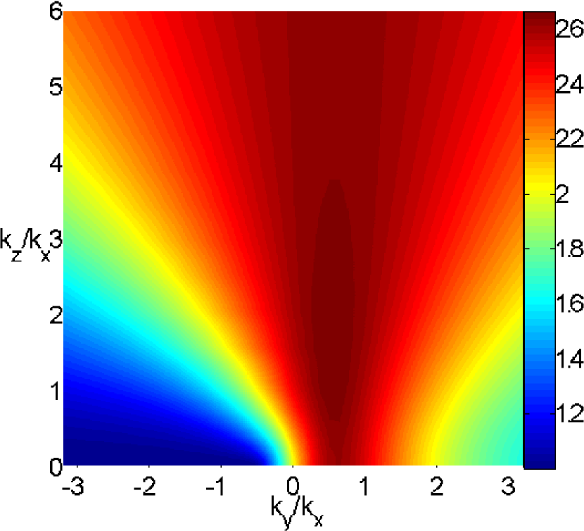
Figure 1: (Color online) Transient growth factor of optimal harmonics’ energy, ${\cal E}_{k}(t_{d})/{\cal E}_{k}(0)$, as a function of wavenumber ratios. It is calculated during the dynamical time $t_{d}=S^{-1}$ with the linearized equations of motion.

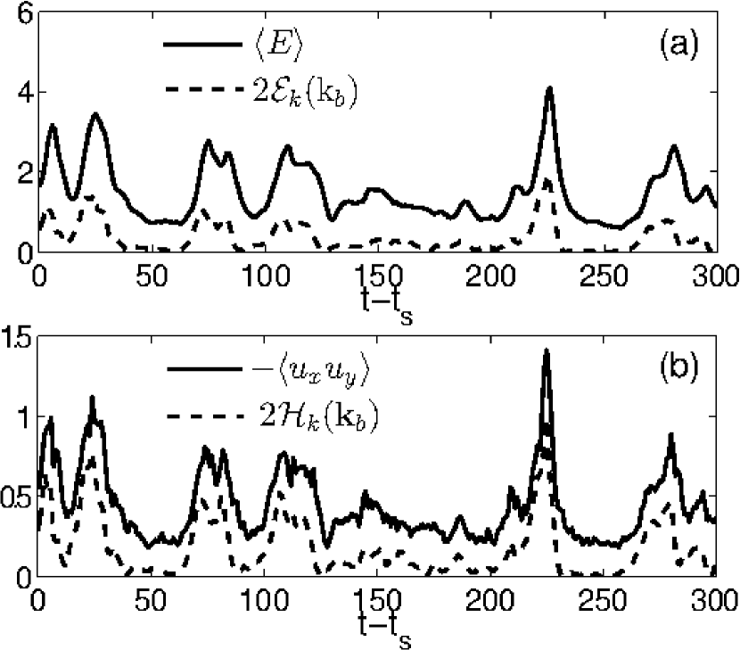
Figure 2: Evolution of (a) the volume-averaged total kinetic energy, $\langle E\rangle$, and the energy of the basic mode with ${\bf k}_{b}=(0,0,\pm 1)$, $2{\cal E}_{k}({\bf k}_{b})$, as well as (b) the volume-averaged Reynolds stress, $-\langle u_{x}u_{y}\rangle$ and the stress corresponding to the basic mode, $2{\cal H}_{k}({\bf k}_{b})$, in the cubic box.

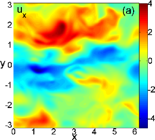
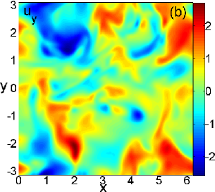
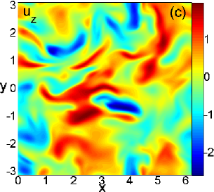
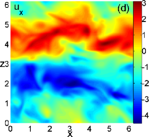
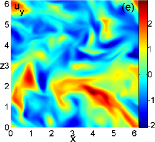
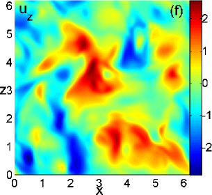
Figure 3: (Color online) Distribution of the velocity components in the fully developed turbulence (at $t-t_{s}=33$) in the cubic box. Shown are $(x,y)$- and $(x,z)$-slices at $z=\pi$ and $y=0$, respectively. The streamwise component $u_{x}$ is larger than $u_{y}$ and $u_{z}$. In the $(x,z)$ slices of $u_{y}$ and especially of $u_{x}$, a signature of the basic harmonic with large spanwise scale can be discerned.

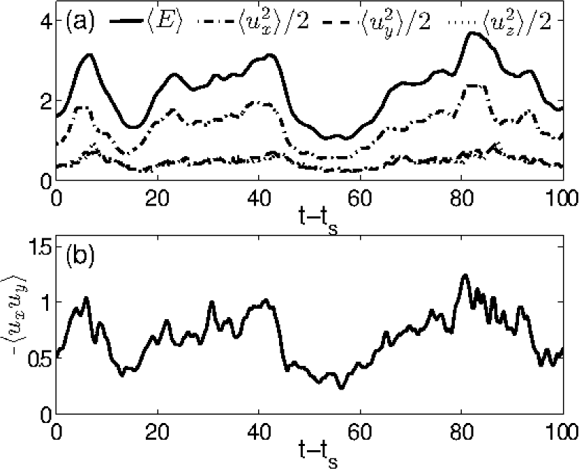
Figure 4: Evolution of (a) the volume-averaged perturbation kinetic energy (solid line) and the quadratic forms of streamwise, $\langle u_{x}^{2}\rangle/2$ (dot-dashed line), shearwise/vertical, $\langle u_{y}^{2}\rangle/2$ (dashed line) and spanwise, $\langle u_{z}^{2}\rangle/2$ (doted line) velocities as well as (b) the Reynolds stress in the cubic box.

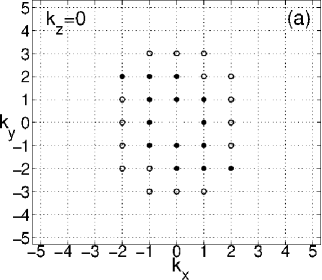
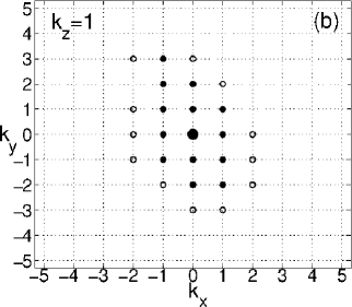
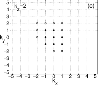
Figure 5: Distribution of the modes carrying dominant energy in k-space at (a) $k_{z}=0$ (b) $k_{z}=1$ and (c) $k_{z}=2$ in the cubic box. Black dots represent the harmonics whose energies grow more than $10\%$ of the maximum spectral energy at least once during evolution. The biggest black dot in the plot (b) corresponds to the basic mode with the maximum spectral energy at all times. Circles represent the harmonics whose energies grow from 5% to 10% of the maximum spectral energy.

It is well-known from the linear nonmodal theory of shear flows that optimal perturbations characterized by a maximum nonmodal growth during the dynamical or eddy turnover time, which can be assumed of the order of shear time, $t_{d}\simeq S^{-1}$ (or, $t_{d}\simeq 1$ in normalized units) are responsible for most of the energy extraction from the background flow Schmid and Henningson (2001); Farrell and Ioannou (1996). Figure 1 shows the growth factor of energy for optimal harmonics calculated from the linearized inviscid equations of motion, i.e., using only the first linear terms on the rhs of Eqs. (13)-(15). These terms, and hence the linear dynamics of harmonics in the inviscid case, depends only on the ratios of wavenumbers, $k_{y}/k_{x}$ and $k_{z}/k_{x}$. It is seen from this figure that the optimal growth factor is largest at $1\lesssim k_{z}/k_{x}<4$ and $0<k_{y}/k_{x}\lesssim 1$. Consequently, one can encompass as many of these optimal perturbations as possible and thus better account for their major role in the energy exchange processes between turbulence and background flow if the computational box aspect ratios satisfy the conditions: $A_{xz}\leq A_{yz}$ and $A_{xz}\geq 1$.

In agreement with the previous study of homogeneous shear turbulence by Pumir Pumir (1996), in our simulations we found that in addition to the non-symmetric ($k_{x}\neq 0$) optimal harmonics, a harmonic with a large scale spanwise variation, which is uniform in the streamwise and shearwise directions, $k_{x}=k_{y}=0,k_{z}=\pm 1$, plays a central role in the turbulence dynamics. Due to its importance, we call this harmonic the basic mode. Other harmonics, whose energy grows more than 10% of the maximum value of the spectral energy at least once during the evolution, are considered to be actively participating in and forming the self-sustaining dynamics of turbulence. In particular, we show that one of the characteristic features of the homogeneous shear turbulence – quasi-periodic bursts of energy and Reynolds stress Pumir (1996) – are determined by a competition between the basic mode and other dynamically “active” harmonics, whose number generally depends on the box aspect ratio and is usually large.

Below we focus on three different boxes with the following aspect ratios: $(A_{xz},A_{yz})=(1,1)$ (cubic box), $(3,2)$, $(1,2)$ and analyze in detail the specific spectra and self-sustaining dynamics of turbulence in wavenumber/spectral space by calculating the Fourier transforms of individual linear and nonlinear terms in governing equations using the DNS data. In all simulations, the time-averages of the spectral quantities are calculated over an entire time of the saturated turbulent state, discarding an initial transient phase, which typically lasts for about $30S^{-1}$.

III.1 Aspect ratio $(A_{xz},A_{yz})=(1,1)$

At the early stage of evolution, each harmonic contained in the initial perturbations grows due to the flow nonnormality, leading to the growth of the total energy and Reynolds stress. Then, after about $t_{s}=30S^{-1}$, the amplitudes of the perturbations become sufficiently large in the nonlinear regime and eventually the flow settles into a self-sustained turbulence. In this cubic box, the basic mode/harmonic with wavenumber ${\bf k}_{b}=(0,0,\pm 1)$, dominates over other ones, i.e., its spectral energy, ${\cal E}_{k}({\bf k}_{b})$, and stress, ${\cal H}_{k}({\bf k}_{b})$, are, respectively, maximum of ${\cal E}_{k}$ and ${\cal H}_{k}$ during an entire course of evolution (see also Ref. Pumir (1996)). Figure 2 shows the evolution of the volume-averaged total energy and stress as well as the energy and stress of the basic mode in the saturated state, which display similar patterns of quasi-periodic bursts in time. The volume-averaged Reynolds stress (with negative sign), $-\langle u_{x}u_{y}\rangle$, and the stress of the basic mode, ${\cal H}_{k}({\bf k}_{b})$ are positive at all times and non-decaying as required by the self-sustaining process according to Eq. (8). The bursts in the total energy and stress closely follow amplifications (peaks) of ${\cal E}_{k}({\bf k}_{b})$ and stress ${\cal H}_{k}({\bf k}_{b})$ in the basic mode. This indicates that these bursts are related to the dynamics of the basic mode, which thus appears to be mainly responsible for the energy pumping from the background flow into turbulence. During the bursts, the contribution of ${\cal H}_{k}({\bf k}_{b})$ to the total Reynolds stress is as much as 60% - 70%, while other modes become significant, although still remain smaller than the basic mode, in quiescent intervals between the bursts, when the total energy and stresses as well as the energy and stress of the basic mode are low. So, for the aspect ratio $(1,1)$, most of the turbulent energy is produced through the interaction of the basic mode with the background shear flow.

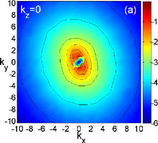
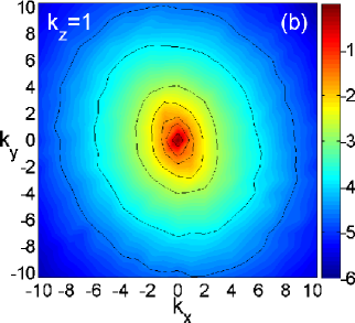
Figure 6: (Color online) Logarithm of the time-averaged spectrum of the kinetic energy, $log_{10}({\cal E}_{k})$, in the cubic box. The $(k_{x},k_{y})$-slices are at (a) $k_{z}=0$, (b) $k_{z}=1$ and (c) $k_{z}=2$. The spectrum has an anisotropic character, having larger power in the $k_{y}/k_{x}<0$ part of Fourier space at a given $k_{x}$. The spectral energy has maximum at $k_{z}=1$ and decreases with increasing $k_{z}$.

Figure 7: Integrated in $(k_{x},k_{y})$-plane time-averaged (a) kinetic energy spectrum, $\hat{\cal E}$, and (b) Reynolds stress, $\hat{\cal H}$ vs. $k_{z}$.

The structure of the velocity components in the fully developed turbulence in physical space is presented in Fig. 3. The evolution of the volume-averaged perturbation kinetic energy and quadratic forms of streamwise, $\langle u_{x}^{2}\rangle/2$, shearwise/vertical, $\langle u_{y}^{2}\rangle/2$, and spanwise, $\langle u_{z}^{2}\rangle/2$, velocities as well as the Reynolds stress are shown in Fig. 4. From these plots it is clear that the streamwise velocity prevails over the shearwise and spanwise ones. In the $(x,z)$ slices of $u_{y}$ and, especially, of $u_{x}$, we clearly see the signatures of the dominant basic harmonic with small scale fluctuations due to other harmonics superimposed on it.

To understand the role of other modes in the turbulence dynamics, it is important to define the main, energy-containing area in k-space, which we also refer to as the vital area of turbulence. For this purpose we define two sets of harmonics whose energy grows from 5% to 10% and those larger than 10% of the maximum spectral energy at least once during the evolution; the second set is referred to as “active modes”. These energy-carrying, or dynamically important harmonics are displayed in Fig. 5. They have small wavenumbers $|k_{x}|\leq 2,|k_{y}|\leq 3,|k_{z}|\leq 3$, which basically form the vital area of turbulence (at $k_{z}=3$, not shown in this figure, mode energies always remain less than 10% of the maximum energy). Harmonics with larger wavenumbers $|k_{x}|>2,|k_{y}|>3,|k_{z}|>3$ lie outside the vital area and always have energy and stress less than 5% of the maximum value, therefore, not playing a major role in the energy exchange process between the background flow and turbulence. Essentially, only these large scale modes in the vital area take part in the self-sustaining dynamics of turbulence, but the basic mode/harmonic still remains dominant – it is the most active among the active harmonics. We emphasize that the total number of the large scale active modes (black dots in Fig. 5) is equal to 36, implying that the dynamics of homogeneous shear turbulence cannot be reduced to low-order models of the self-sustaining processes.

Figure 6 shows the time-averaged spectrum of the kinetic energy in $(k_{x},k_{y})$-plane at different $k_{z}$. The spectrum is anisotropic due to shear – the isolines have elliptical shape inclined opposite to the $k_{y}$-axis. This fact indicates that on average modes with $k_{y}/k_{x}<0$ have more energy than those with $k_{y}/k_{x}>0$ at fixed $k_{x}$. The plots show that the time-averaged spectral kinetic energy at fixed $k_{z}$ is larger for small $k_{x}$ and $k_{y}$ and decays at least by two order of magnitude at $\sqrt{k_{x}^{2}+k_{y}^{2}}\approx 2$. So, the active modes are located just within this range of small wavenumbers, as also seen in Fig. 5. As mentioned above, the maximum of the spectral energy is reached at $k_{x}=k_{y}=0,k_{z}=\pm 1$ corresponding to the basic mode. However, it decays significantly already for the next spanwise modes with $k_{z}=2$ and further decreases rapidly with increasing $k_{z}$. This behavior is also seen in Fig. 7, which shows the integrated in $(k_{x},k_{y})$-plane the time-averaged spectral energy, $\hat{\cal E}(k_{z})=\int{\cal E}_{k}dk_{x}dk_{y}$, and stress, $\hat{\cal H}(k_{z})=\int{\cal H}_{k}dk_{x}dk_{y}$, vs. $k_{z}$. Both reach a maximum at $k_{z}=\pm 1$ and rapidly decrease with $|k_{z}|$.

The anisotropic nature of the kinetic energy spectrum, which clearly distinguishes it from the isotropic spectrum in the classical (without shear) Kolmogorov phenomenology, arises as a result of the specific action of linear and nonlinear processes in k-space. As we show below, these processes are anisotropic over wavenumbers due to shear, resulting in a new phenomenon – the transverse redistribution of power in spectral space.

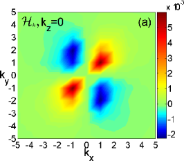
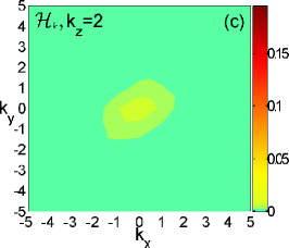
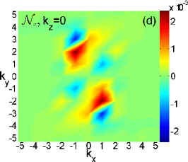
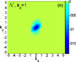
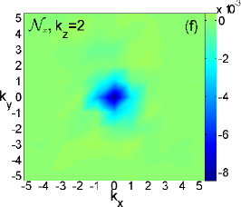
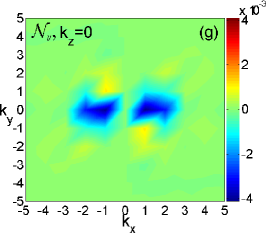
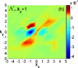
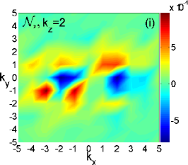
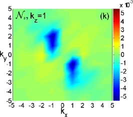
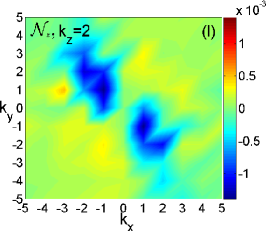
Figure 8: (Color online) Maps of the time-averaged energy injecting stress [(a), (b), (c)], ${\cal H}_{k}$, and nonlinear transfer, [(d), (e), (f)] ${\cal N}_{x}$, [(g), (h), (i)] ${\cal N}_{y}$, [(j), (k), (l)] ${\cal N}_{z}$ functions in k-space for the cubic box. Shown are $(k_{x},k_{y})$-slices of these quantities at $k_{z}=0$ (left column), $k_{z}=1$ (middle column) and $k_{z}=2$ (right column). ${\cal H}_{k}$ is significant in the vital area $|k_{x}|\leq 2,|k_{y}|\leq 3,|k_{z}|\leq 2$, on the $k_{y}/k_{x}>0$ side. Hence, the energy injection into turbulence mainly occurs in this region. At $k_{z}=1$, ${\cal H}_{k}$ reaches largest values and consequently energy injection is most intensive at this wavenumber. ${\cal N}_{x}$, ${\cal N}_{y}$ and ${\cal N}_{z}$ transfer, respectively, the streamwise, shearwise and spanwise components of the spectral kinetic energy anisotropically, or transversely over wavevector angles in Fourier space, away from the regions where they are negative ${\cal N}_{x}<0,~{}{\cal N}_{y}<0,~{}{\cal N}_{z}<0$ (blue) towards the regions where they are positive ${\cal N}_{x}>0,~{}{\cal N}_{y}>0,~{}{\cal N}_{z}>0$ (yellow and red).

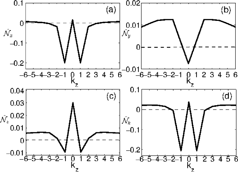
Figure 9: The time-averaged nonlinear transfer functions integrated in $(k_{x},k_{y})-$plane and represented as a function of $k_{z}$, (a) $\hat{\cal N}_{x}$, (b) $\hat{\cal N}_{y}$, (c) $\hat{\cal N}_{z}$ and their sum (d) $\hat{\cal N}_{k}$ describing nonlinear transfer of energy. These functions transfer corresponding quantities from $k_{z}$ at which they are negative to those $k_{z}$ at which they are positive.

Energy injection, nonlinear transfers and their interplay in ${\bf k}$-space

To understand the origin of the anisotropic character of the energy spectrum, in Fig. 8 we present the distribution of the time-averaged energy-injecting Reynolds stress spectrum, ${\cal H}_{k}$, and the nonlinear transfer functions, ${\cal N}_{x},{\cal N}_{y}$ and ${\cal N}_{z}$, in k-space. Since these quantities are symmetric with respect to a change ${\bf k}\rightarrow-{\bf k}$, without loss of generality, hereafter we concentrate on the upper part ($k_{z}\geq 0$) of k-space. First of all, these plots clearly demonstrate the anisotropic nature of the linear and nonlinear processes in k-space – all these quantities exhibit anisotropy over wavenumbers, that is, depend on wavevector angle, or orientation. ${\cal H}_{k}$ is significant primarily in the vital area of spectral space, $|k_{x}|\leq 2,|k_{y}|\leq 3,|k_{z}|\leq 2$, at $k_{y}/k_{x}>0$, where it supplies the turbulence with energy via nonmodal growth of the dynamically active modes (see below). At $k_{z}=0$, ${\cal H}_{k}$ is mainly concentrated around $|k_{y}|,|k_{x}|\sim 1$ [Fig. 8(a)], it is positive at $k_{x}/k_{y}>0$, supplying harmonics with energy and negative at $k_{x}/k_{y}<0$, returning energy to the flow. On the other hand, at $k_{z}\geq 1$, the distribution of ${\cal H}_{k}$ is changed – it is positive and achieves local maximum around $k_{x}=k_{y}=0$ at each $k_{z}$ [Figs. 8(b) and 8(c)]. The Reynolds stress spectrum is highest and therefore the energy extraction from the background flow into turbulence more effectively occurs for modes with $k_{z}=\pm 1$, reaching the maximum at ${\bf k}_{b}$ corresponding to the basic mode [Figs. 8(b), see also Fig. 7(b)]. Outside the vital area, at $|k_{x}|>2,|k_{y}|>3,|k_{z}|>2$, the stress and hence the energy input into turbulence rapidly decrease and vanish at large wavenumbers. The total energy input at $k_{z}=0$ is also negligible, $\hat{\cal H}\approx 0$, as seen from Fig. 7(b), since ${\cal H}_{k}$ changes sign in $(k_{x},k_{y})$-plane at this $k_{z}$ [Fig. 8(a)]. Thus, the main energy supply for turbulence is due to large-scale modes with the wavelengths comparable to the box size. Note that the energy injection into turbulence mediated by the stress occurs over a range wavenumbers and in this respect differs from the classical cases of forced turbulence in flows without shear, where forcing is applied at a specific wavenumber or a narrow range of wavenumbers (see e.g., Biskamp (2003)).

The nonlinear transfer functions ${\cal N}_{x},{\cal N}_{y},{\cal N}_{z}$ [Figs. 8(d)-8(l)] depend on wavevector angle and, consequently, redistribute the streamwise, shearwise and spanwise velocity energies generally not only along wavevector (direct/inverse cascades), but also transverse to wavevector. The latter occurs away from the regions in k-space where the respective transfer functions are negative ${\cal N}_{x},{\cal N}_{y},{\cal N}_{z}<0$ [blue areas in Figs. 8(d)-8(l)] to regions where they are positive ${\cal N}_{x},{\cal N}_{y},{\cal N}_{z}>0$ (yellow and red areas); at all other wavenumbers (light green areas) these functions are small. It is seen from Figs. 8(d)-8(l) that this transverse cascade primarily operates within the vital area of the wavenumber space, $|k_{x}|\leq 2,|k_{y}|\leq 3,|k_{z}|\leq 2$, where the nonnormality-induced energy exchange between the background flow and harmonics is dominant. Outside the vital area at large wavenumbers, the transfer functions become nearly independent of the wavevector angle and depend mostly on its magnitude, i.e., the cascade is not transverse anymore but direct. So, outside the vital area the situation is similar to the classical homogeneous isotropic turbulence described by Kolmogorov phenomenology. To characterize transfers along $k_{z}$, we integrate ${\cal N}_{i}$ over $(k_{x},k_{y})$-plane, $\hat{\cal N}_{i}(k_{z})=\int{\cal N}_{i}dk_{x}dk_{y},(i=x,y,z,k)$, and represent them as functions of $k_{z}$ in Fig. 9.

The interplay between the energy-injecting linear process and the transverse cascade determines the self-sustaining dynamics of turbulence and characteristics of the energy spectrum in the presence of shear. Figures 8(d)-8(f) and 9(a) show that ${\cal N}_{x}$ is negative and large by absolute value in the vital area, where the stress, ${\cal H}_{k}$, is positive and appreciable. Outside the vital area, i.e., at larger wavenumbers ($|k_{x}|>2,|k_{y}|>3,|k_{z}|\geq 3$), ${\cal N}_{x}$ is positive but small and the stress is also negligibly small. In other words, ${\cal N}_{x}$ provides a sink, or negative feedback for ${\cal H}_{k}$ by taking out energy in the streamwise velocity gained from the background flow and transferring it to large wavenumbers and part of it to $k_{z}=0$, as evident from the dependence of ${\cal{\hat{N}}}_{x}$ on $k_{z}$. By contrast, ${\cal N}_{y}$ is positive in those regions of the vital area where ${\cal H}_{k}$ is also positive [Figs. 8(g)-8(i) and 9(b)]. As a result, it provides positive feedback at these wavenumbers by generating the shearwise energy, $|\bar{u}_{y}|^{2}/2$, which, in turn, leads to the growth of the streamwise energy, $|\bar{u}_{x}|^{2}/2$, due to the linear nonmodal growth mechanism (the first terms of linear origin on the rhs of Eqs. 13 and 16, while ${\cal N}_{x}<0$ at these wavenumbers and cannot contribute to the growth). The streamwise energy, which in fact appears to be largest among the other two components, is then transferred to larger wavenumbers by ${\cal N}_{x}$. Note that this positive feedback due to ${\cal N}_{y}$ is crucial to the self-sustenance of turbulence and is realized by the transverse cascade, which ensures supply of the shearwise energy for harmonics with such wavevector orientations ($k_{y}/k_{x}>0$) that correspond to positive stress ${\cal H}_{k}>0$ and hence with the capability of nonmodal growth. Figures 8(j)-8(l) and 9(c) show ${\cal N}_{z}$, which is responsible for the transfer of energy in the spanwise velocity. However, since the Reynolds stress providing energy supply for the turbulence is produced by the product (correlation) of $u_{x}$ and $u_{y}$, below we concentrate only on ${\cal N}_{x}$ and ${\cal N}_{y}$ that govern nonlinear redistribution of these velocity components. Figure 9(d) shows the nonlinear transfer function for the energy, $\hat{\cal N}_{k}=\hat{\cal N}_{x}+\hat{\cal N}_{y}+\hat{\cal N}_{z}$. It is dominated by $\hat{\cal N}_{x}$ and hence the nonlinear transfer of the total energy over wavenumbers is similar to that of the streamwise energy.

Thus, the transverse cascade of energy appears to be a generic feature of nonlinear dynamics of perturbations in spectrally stable shear flows. The conventional description of shear flow turbulence solely in terms of direct and inverse cascades, which leaves such nonlinear transverse cascade out of consideration, might be incomplete and misleading. It should be emphasized that revealing the complete picture of these nonlinear cascade processes has become largely possible due to carrying out the analysis in Fourier space. Because of the shear-induced anisotropy of cascade directions, often used energy spectra and transfer functions integrated, or averaged over wavevector angles, clearly, are not fully representative of the actual, more general (transverse) redistribution of the spectral energies due to nonlinearity in k-space.

We have described above the linear and nonlinear process in a time-average sense in the fully developed turbulence. To gain a better insight in its self-sustenance and appearance of the bursts in the total energy evolution (Fig. 2), below we analyze the temporal evolution of individual harmonics in the vital area for fixed $k_{x},k_{y},k_{z}$.

First we consider the dynamics of the dominant basic mode with ${\bf k}_{b}=(0,0,\pm 1)$, which corresponds to the maximum energy and stress in spectral space during the whole evolution in the case of the cubic box. For this mode, the dynamical Eqs. (16)-(18) are reduced to the following system ($S=1$ everywhere below):

$$\frac{\partial}{\partial t}\frac{|\bar{u}_{x}({\bf k}_{b},t)|^{2}}{2}={\cal H}_{k}({\bf k}_{b},t)+{\cal N}_{x}({\bf k}_{b},t)-\nu|\bar{u}_{x}({\bf k}_{b},t)|^{2},$$ (21)

$$\frac{\partial}{\partial t}\frac{|\bar{u}_{y}({\bf k}_{b},t)|^{2}}{2}={\cal N}_{y}({\bf k}_{b},t)-\nu|\bar{u}_{y}({\bf k}_{b},t)|^{2},$$ (22)

$$\frac{\partial}{\partial t}\frac{|\bar{u}_{z}({\bf k}_{b},t)|^{2}}{2}=-\nu|\bar{u}_{z}({\bf k}_{b},t)|^{2}.$$ (23)

Note that ${\cal N}_{z}({\bf k}_{b},t)=0$ and Eq. (23) can be solved analytically, $\bar{u}_{z}({\bf k}_{b},t)=\bar{u}_{z}({\bf k}_{b},0)\exp(-2\nu t)$. Thus, the spanwise velocity decays exponentially in time and the velocity field of the basic harmonic becomes 2D. Figure 10 shows the evolution of the spectral energies of the streamwise and shearwise velocities, $|\bar{u}_{x}({\bf k}_{b})|^{2}/2$, $|\bar{u}_{y}({\bf k}_{b})|^{2}/2$, and the nonlinear transfer functions ${\cal N}_{x}({\bf k}_{b})$, ${\cal N}_{y}({\bf k}_{b})$ for the basic mode. Because the basic mode is of large scale and the Reynolds number is high, the dissipation terms in these equations are negligible. The velocities exhibit a sequence of amplifications (bursts) and decays, with the streamwise velocity being always much larger than the shearwise one. ${\cal N}_{x}({\bf k}_{b})$ is always negative and therefore acts as a sink in the streamwise velocity evolution Eq. (21), while ${\cal N}_{y}({\bf k}_{b})$ oscillates irregularly with alternating sign. When ${\cal N}_{y}({\bf k}_{b})$ is positive, it amplifies the shearwise velocity, while when negative causes its decrease, but the time-average of ${\cal N}_{y}({\bf k}_{b})$ is positive, though small [see also Fig. 8(h)], indicating the growth trend of the shearwise velocity on average. The shearwise velocity generated by ${\cal N}_{y}({\bf k}_{b})$, in turn, leads to the amplification of the streamwise velocity due to the shear-related first linear term on the rhs of dynamical Eq. (13), or equivalently, to the amplification of the streamwise energy due to the stress term ${\cal H}_{k}({\bf k}_{b})$ in Eq. (21). Note that this is the only cause of amplification for $|\bar{u}_{x}({\bf k}_{b})|$, since the corresponding nonlinear term, ${\cal N}_{x}({\bf k}_{b})$, is always negative and cannot amplify it. Then, $\bar{u}_{y}({\bf k}_{b})$ and the amplified $\bar{u}_{x}({\bf k}_{b})$ jointly give rise to positive stress, ${\cal H}_{k}({\bf k}_{b})>0$ [Figs. 2(b) and 11(b)]. As a result, the stress production rate, $d{\cal H}_{k}({\bf k}_{b})/dt$ (calculated by combining Eqs. 13 and 14), closely follows, or correlates with ${\cal N}_{y}({\bf k}_{b})$ [Fig. 11(a), the correlation coefficient is $R(d{\cal H}_{k}/dt,{\cal N}_{y})=0.93$,] and, consequently, the stress itself follows $|\bar{u}_{y}({\bf k}_{b})|$ [Fig. 11(b), $R({\cal H}_{k},|\bar{u}_{y}|)=0.97$], i.e., the peaks, or bursts and dips in the temporal evolution of these quantities coincide. So, the transfer function ${\cal N}_{y}({\bf k}_{b})$ plays a central role in the dynamics of the basic mode by providing a positive feedback to the linear nonmodal growth: when ${\cal N}_{y}({\bf k}_{b})>0$, it causes the amplification of $\bar{u}_{y}({\bf k}_{b})$, which via nonmodal growth mechanism leads in turn to the amplification of $\bar{u}_{x}({\bf k}_{b})$ and hence of the corresponding stress. These growth intervals in the evolution of these quantities alternate with the decaying intervals where ${\cal N}_{y}({\bf k}_{b})<0$. Since for the aspect ratio $(1,1)$, the basic mode is the dominant one among all the active modes, these bursts also manifest themselves in the total stress evolution, as is seen in Fig. 2(b).

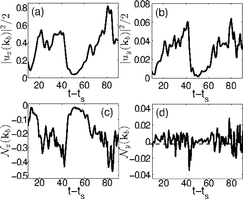
Figure 10: Evolution of (a) the streamwise, $|\bar{u}_{x}({\bf k}_{b})|^{2}/2$, and (b) shearwise, $|\bar{u}_{y}({\bf k}_{b})|^{2}/2$, spectral energies as well as the nonlinear transfer functions (c) ${\cal N}_{x}({\bf k}_{b})$ and (d) ${\cal N}_{y}({\bf k}_{b})$ for the basic mode with ${\bf k}_{b}=(0,0,\pm 1)$ in the cubic box. The streamwise energy is much larger than the shearwise one due to the linear nonmodal growth process. ${\cal N}_{x}({\bf k}_{b})$ is negative during the whole evolution, acting as a sink for the streamwise energy, while ${\cal N}_{y}({\bf k}_{b})$ oscillates and, when positive, causes increase in $|\bar{u}_{y}|$; its time-averaged value over the evolution is positive $4.78\cdot 10^{-4}$.

Figure 11: Evolution of (a) the stress production rate, $d{\cal H}_{k}({\bf k}_{b})/dt$, and nonlinear transfer term ${\cal N}_{y}({\bf k}_{b})$ as well as (b) the spectral Reynolds stress, ${\cal H}_{k}({\bf k}_{b})$, and shearwise velocity, $|\bar{u}_{y}({\bf k}_{b})|$ of the basic mode in the cubic box. The stress production rate closely follows ${\cal N}_{y}({\bf k}_{b})$ (which is scaled by a factor of 2 to make comparison easier) and, consequently, the amplifications (bursts) of both shearwise velocity and stress occur when ${\cal N}_{y}({\bf k}_{b})$ is positive and decrease when this term is negative.

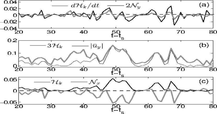
Figure 12: Evolution of (a) the stress production rate and nonlinear transfer term ${\cal N}_{y}$, (b) the stress ${\cal H}_{k}$ and shearwise velocity $|\bar{u}_{y}|$ and (c) the stress and ${\cal N}_{x}$ for the mode ${\bf k}_{1}=(0,1,1)$. The nonlinear function in (a) and the stress in (b) are scaled by 2 and 3, respectively, for the sake of comparison.

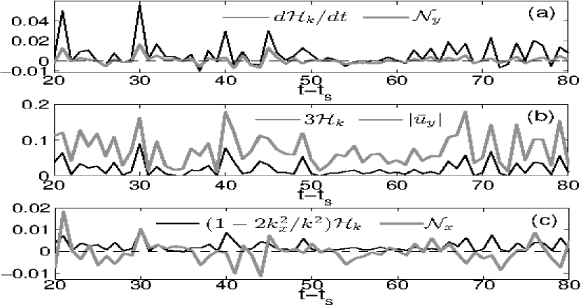
Figure 13: Same as in Fig. 12, but for the non-symmetric mode ${\bf k}_{2}=(1,1,1)$. The stress in (b) is scaled by a factor of 3. A high degree of correlation exists between the stress production rate and the nonlinear term ${\cal N}_{y}$ (a) as well as the stress and shearwise velocity (b), implying that the stress amplification is due to the nonmodal growth of $\bar{u}_{x}$ from $\bar{u}_{y}$.

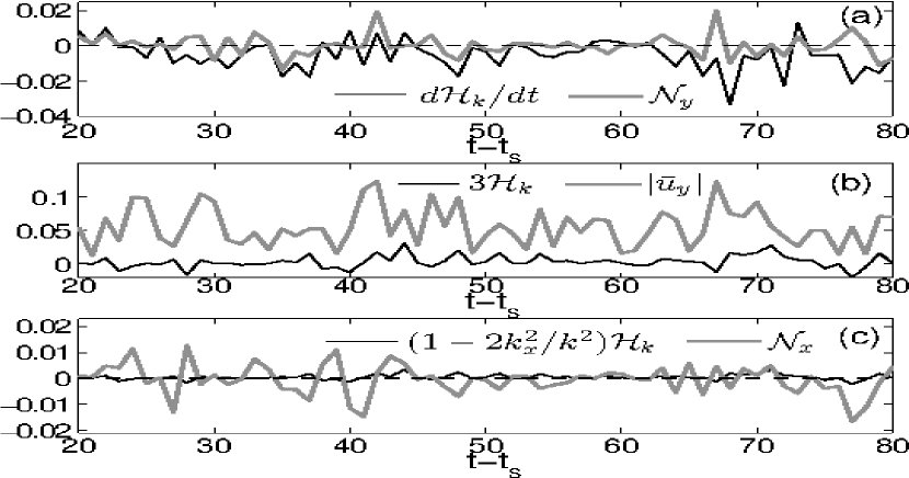
Figure 14: Same as in Fig. 13, but for the mode ${\bf k}_{3}=(1,-1,1)$. The stress in (b) is scaled by a factor of 3. Unlike the modes in Figs. 12 and 13, ${\cal N}_{x}$ dominates the nonnormality/shear-induced linear term and consequently the stress and shearwise velocity do not correlate for this harmonic. The corresponding stress is smaller than those of the other two modes.

The same nonmodal linear growth and nonlinear processes underlie the dynamics of other symmetric ($k_{x}=0$) and non-symmetric ($k_{x}\neq 0$) active modes in the vicinity of ${\bf k}_{b}$ within the vital area (Fig. 5), however, their quantitative character depends on mode wavenumbers. To demonstrate this, in Figs. 12-14 we show the dynamics for such nearby symmetric mode with ${\bf k}_{1}=(0,1,1)$ and non-symmetric modes with ${\bf k}_{2}=(1,1,1)$ and ${\bf k}_{3}=(1,-1,1)$. These figures display the time-history of (a) the stress production rate $d{\cal H}_{k}/dt$ and the nonlinear transfer term ${\cal N}_{y}$, (b) stress ${\cal H}_{k}$ and the absolute value of the shearwise velocity, $|\bar{u}_{y}|$, (c) the first shear-induced term of linear origin, $(1-2k_{x}^{2}/k^{2}){\cal H}_{k}$, on the rhs of Eq. (16) and the nonlinear transfer term ${\cal N}_{x}$. We focus on these harmonics with $k_{z}=1$, because, as noted above, they correspond to higher levels of stress and energy than those at other values of $k_{z}$ (Fig. 7), and hence contribute most to the turbulence dynamics. The time-development of the symmetric harmonic with ${\bf k}_{1}$ (Fig. 12) is similar to that of the basic mode except that it has much less energy and stress. It is again governed by Eqs. (21) and (22) (with ${\bf k}_{b}$ replaced by ${\bf k}_{1}$), but since ${\cal N}_{z}({\bf k}_{1})$ is no longer zero, it generates the spanwise velocity, which, although does not contribute to the stress, takes up part of the mode’s energy. The stress production rate and ${\cal N}_{y}({\bf k}_{1})$ evolve nearly similarly with time [Fig. 12(a)], though with a bit lesser correlation $R(d{\cal H}_{k}/dt,{\cal N}_{y})=0.78$ than that in the case of the basic mode. Therefore, the stress ${\cal H}_{k}({\bf k}_{1})$ and the shearwise velocity, $|\bar{u}_{y}({\bf k}_{1})|$, also display similar behavior in time with coinciding amplification and decay intervals [Fig. 12(b), $R({\cal H}_{k},|\bar{u}_{y}|)=0.86$]. Figure 12(c) shows that the stress remains positive at all times and supplies the mode with energy, while ${\cal N}_{x}({\bf k}_{1})$ is negative and acts as a sink for the energy of the streamwise velocity. This indicates again that ${\cal N}_{y}$ represents the only source maintaining the shearwise velocity and hence the stress.

The linear nonmodal dynamics for the non-symmetric harmonics is described by the terms of linear origin related to shear in the above dynamical equations in Fourier space. First consider the non-symmetric mode with ${\bf k}_{2}$ (Fig. 13). For this mode, ${\cal N}_{y}({\bf k}_{2})$ acts as a source and generates the shearwise velocity, $|\bar{u}_{y}({\bf k}_{2})|$. The latter is then nonmodally amplified due to the first linear shear-induced term on the right hand side of Eq. (17), $k_{x2}k_{y2}|\bar{u}_{y}({\bf k}_{2})|^{2}/k_{2}^{2}$, which is always positive for this mode since $k_{x2}k_{y2}>0$. Because ${\cal N}_{y}({\bf k}_{2})$ is also positive on average in time [see Fig. 8(h)], the linear and nonlinear terms in this equation cooperate with each other in the growth of $|\bar{u}_{y}({\bf k}_{2})|$. During its amplification, the shearwise velocity generates and nonmodally amplifies the streamwise velocity, $\bar{u}_{x}({\bf k}_{2})$, due to the first shear-related linear term on the rhs of Eq. (13), or equivalently, by the $(1-2k_{x2}^{2}/k_{2}^{2}){\cal H}_{k}({\bf k}_{2})$ term on the rhs of Eq. (16). As seen from Fig. 13(c), ${\cal N}_{x}({\bf k}_{2})$ is negative most of the time (and hence on average) for this harmonic and therefore acts as a sink for $|\bar{u}_{x}({\bf k}_{2})|$, opposing its growth. $\bar{u}_{x}$ and $\bar{u}_{y}$ velocity components give rise to the stress ${\cal H}_{k}({\bf k}_{2})$, whose production rate, as a result, correlates with ${\cal N}_{y}({\bf k}_{2})$ in time [Fig. 13(a), $R(d{\cal H}_{k}/dt,{\cal N}_{y})=0.84$]. Due to this, the temporal evolution of ${\cal H}_{k}({\bf k_{2}})$ itself closely correlates with $|\bar{u}_{y}({\bf k}_{2})|$ [Fig. 13(b), $R({\cal H}_{k},|\bar{u}_{y}|)=0.9$]. So, increase (decrease) of ${\cal N}_{y}({\bf k}_{2})$ results in the increase (decrease) of the stress production rate. Consequently, the increase (decrease) in the shearwise velocity leads to the increase (decrease) in the stress and hence in the energy extraction from the flow. It is clear from Figs. 13(a) and 13(b) that the peaks, respectively, in the evolution of ${\cal N}_{y}({\bf k}_{2})$ and $d{\cal H}_{k}({\bf k}_{2})/dt$ and in the evolution of $|\bar{u}_{y}({\bf k}_{2})|$ and ${\cal H}_{k}({\bf k}_{2})$ coincide. We note that these high correlations, leading to the growth of the Reynolds stress, are related to the fact that $\bar{u}_{x}({\bf k}_{2})$ grows from $\bar{u}_{y}({\bf k}_{2})$ due to nonnormality/shear (first term on the rhs of Eq. 13), whereas $\bar{u}_{y}({\bf k}_{2})$ is produced by the nonlinear transfer term ${\cal N}_{y}({\bf k}_{2})$. The nonmodal growth mechanism, as for the basic mode, also for this non-symmetric mode ensures that streamwise and shearwise velocities correlate such that the resulting Reynolds stress remains positive, ${\cal H}_{k}({\bf k}_{2})>0$, at all times [Fig. 13(b)], which is necessary for the continual extraction of energy from the background flow into the harmonic. This is the essence of the interplay between nonlinearity, which generates seed shearwise velocity, and the nonmodal growth process that generates and amplifies streamwise velocity from the shearwise one and ultimately the positive stress.

The situation is different for the mode with ${\bf k}_{3}=(1,-1,1)$ (Fig. 14). The stress and shearwise velocity are not related – the corresponding correlation coefficients are much smaller than those in the previous cases, $R(d{\cal H}_{k}/dt,{\cal N}_{y})=0.17$, $R({\cal H}_{k},|\bar{u}_{y}|)=0.24$. The first shear-induced linear term on the rhs of Eq. (16), responsible for the nonmodal growth of the streamwise velocity, is dominated by ${\cal N}_{x}({\bf k}_{3})$ [Fig. 14(c)]. As a result, the evolution of $|\bar{u}_{x}({\bf k}_{3})|$ is governed mainly by ${\cal N}_{x}({\bf k}_{3})$, and the effect of the nonnormality is small. Moreover, in contrast to the harmonic with ${\bf k}_{2}$, the term responsible for the nonmodal growth of the shearwise velocity is always negative, $k_{x3}k_{y3}|\bar{u}_{y}({\bf k}_{3})|^{2}/k_{3}^{2}<0$, and opposes ${\cal N}_{y}({\bf k}_{3})$ in the amplification of $|\bar{u}_{y}({\bf k}_{3})|$. In other words, for the shearwise velocity, there is no constructive interplay between nonnormality-induced linear dynamics and the nonlinear term. So, the production rate of the streamwise velocity at ${\bf k}_{3}$ is much reduced compared to that for ${\bf k}_{2}$. This leads to the absence of correlation between the temporal evolution of the stress production rate and ${\cal N}_{y}({\bf k}_{3})$ [Fig. 14(a)] and hence between the stress ${\cal H}_{k}({\bf k}_{3})$ and shearwise velocity [Fig. 14(b)]. Since $|\bar{u}_{x}({\bf k}_{3})|$ is determined mainly by the nonlinear transfer term ${\cal N}_{x}({\bf k}_{3})$ rather than by the nonmodal dynamics, it is not correlated with $\bar{u}_{y}({\bf k}_{3})$. As a result, the Reynolds stress produced by these two velocity components is irregularly oscillating between positive and negative values [Fig. 14(b)] in contrast to the basic mode and the ${\bf k}_{1}$ and ${\bf k}_{2}$ modes, whose corresponding stresses are always positive owing to the linear nonmodal growth mechanism [see for comparison Figs. 12(b) and 13(b)]. Because of this, the time-averaged value of the stress corresponding to this mode, being equal to $0.0011$, is smaller than that for the ${\bf k}_{2}$ mode, which is 0.006. So, due to the constructive interplay between the nonlinear and linear terms in the case of the basic mode and ${\bf k}_{1}$ and ${\bf k}_{2}$ modes, their effectiveness in the energy extraction from the background flow is higher than that of the ${\bf k}_{3}$ mode, for which such an interplay is practically absent.

Although the dynamics of only three modes, one symmetric and other two non-symmetric ones with $k_{y}/k_{x}>0$ and $k_{y}/k_{x}<0$ at $k_{z}=1$, were described above, the other neighboring modes in these regions of k-space exhibit a similar dynamics too. The time-averaged plots of Figs. 8(a)-8(c) clearly show that in the vital area, the Reynolds stress of active modes with $k_{y}/k_{x}<0$ on average is smaller than that of ones with $k_{y}/k_{x}>0$, which thus contribute most to the positive stress. They play a key role in supplying turbulence with energy, together with the basic and nearby symmetric modes. These modes share a similar dynamics with the ${\bf k}_{2}$ mode and therefore the higher values of the associated stress are due to a constructive interplay between nonmodal growth and nonlinear feedback discussed above. From these plots we see that on average ${\cal N}_{y}>0$ at $k_{y}/k_{x}>0$ and $k_{x}=0$, indicating that the transverse cascade continually regenerates just these modes, thereby ensuring the self-sustenance of the turbulence.

Figure 15: Evolution of the volume-averaged (a) perturbed total kinetic energy, $\langle E\rangle$, and (b) the energy ${\cal E}_{k}({\bf k}_{b})$ of the basic mode with ${\bf k}_{b}=(0,0,\pm 1)$ as well as the maximum energy in k-space, ${\cal E}_{k,max}$ (dashed line) for the aspect ratio $(3,2)$. The basic mode corresponds to the maximum energy only during large bursts of the spectral energy, while at other times this maximum is achieved by other neighboring active modes [bigger black dots in Figs. 16(a) and 16(b)]. $\langle E\rangle$ approximately follows the maximum spectral energy and therefore the highest peaks are associated with the dominance of the basic mode at these times.

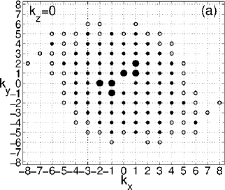
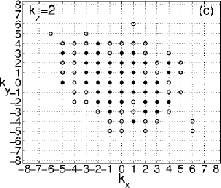
Figure 16: Distribution of the dominant energy-carrying modes in k-space at (a) $k_{z}=0$, (b) $k_{z}=1$ and (c) $k_{z}=2$ during the whole run, for the aspect ratio $(3,2)$. The symbols have the same meaning as in Fig. 5. The bigger black dots represent modes that correspond to the maximum of ${\cal E}_{k}$ at least once during the evolution, including the basic mode at $k_{x}=k_{y}=0,k_{z}=1$.

III.2 Aspect ratio $(A_{xz},A_{yz})=(3,2)$

The evolution of the volume-averaged energy in the saturated turbulence for the aspect ratio $(3,2)$ is shown in Fig. 15(a). It is different from that in the previous case, having weaker and less pronounced bursts. This difference is due to the specific changes of the dynamics in spectral space as the aspect ratio varies. To make a detailed comparison with the previous case, we performed a similar analysis of energy spectra, linear energy-injecting stress and nonlinear transfer terms.

Figure 16 shows the dynamically active, energy-carrying modes during the evolution, as defined above. The number of these modes (209 black dots in Fig. 16) is much larger compared to that in the cubic box. The vital area of turbulence containing these harmonics has become wider in k-space and spans the range $|k_{x}|\leq 8,|k_{y}|\leq 7,|k_{z}|\leq 4$. The basic mode ${\bf k}_{b}=(0,0,\pm 1)$ no longer dominates over the other active modes during the whole evolution, but corresponds to the maximum energy in spectral space only during the highest bursts [Fig. 15(b)]. The lower peaks in the maximum spectral energy curve in Fig. 15(b) are due to symmetric and non-symmetric modes that lie in the vicinity of the basic one in the vital area; these modes are marked by bigger black dots in Figs. 16(a) and 16(b) and have $k_{z}=0,1$. The modes with larger $k_{z}\geq 2$ in the vital area, although being active, never yield maximum of the spectral energy. One can say that the dominance of the basic mode is still retained during the strongest bursts, but because other active modes also reach comparable maximum energies at different times, the bursts in the volume-averaged energy do not appear to be as pronounced as in the cubic box, where only the basic mode prevails over the other active modes at all times.

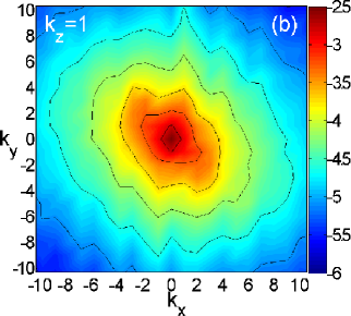
Figure 17: (Color online) Logarithm of the time-averaged kinetic energy spectrum, $log_{10}({\cal E}_{k})$, for the aspect ratio $(3,2)$. The slices in $(k_{x},k_{y})$-plane are at (a) $k_{z}=0$, (b) $k_{z}=1$ and (c) $k_{z}=2$. The spectrum is anisotropic, with larger power at the $k_{y}/k_{x}<0$ side.

Figure 18: Integrated in $(k_{x},k_{y})$-plane time-averaged (a) kinetic energy spectrum, $\hat{\cal E}$, and (b) spectral Reynolds stress, $\hat{\cal H}$, vs. $k_{z}$ for the aspect ratio $(3,2)$. Both the energy and stress achieve their maximum at $k_{z}=\pm 1$, although the energy at $k_{z}=0$ is close to that at $k_{z}=\pm 1$.

Figure 17 shows the time-averaged energy spectrum in $(k_{x},k_{y})$-plane at $k_{z}=0,1,2$. This spectrum is more extended over the wavenumbers compared to that in the cubic box, but has a similar shape and type of anisotropy. Although the maximum of energy is again at $k_{z}=1$, modes with $k_{z}=0$ also have comparable energies, unlike that in the cubic box. As seen from Fig. 16, modes with these two spanwise wavenumbers correspond to the maximum of spectral energy at certain times during evolution and hence play a main role in the turbulence dynamics. The spectral energy then rapidly decreases with increasing $k_{z}$. This behavior is also seen in Fig. 18 showing the time-averaged spectra of the energy and stress integrated in $(k_{x},k_{y})$-plane, $\hat{\cal E}$ and $\hat{\cal H}$. Both these quantities reach their maximum at $k_{z}=\pm 1$. $\hat{\cal E}$ at $k_{z}=0$ is close to its maximum value, while $\hat{\cal H}$ at $k_{z}=0$ is small, because ${\cal H}_{k}(k_{x},k_{y},0)$ changes sign in $(k_{x},k_{y})$-plane, as in the case of the cubic box [see Fig. 8(a)]. So, although harmonics with $k_{z}=0$ can reach energies comparable to those with $k_{z}=1$, in fact, they are not as effective in the net energy extraction from the flow as the latter ones, for which ${\cal H}_{k}$ is positive over the whole $(k_{x},k_{y})$-plane at $k_{z}=1$ [Fig. 19(a)].

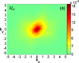
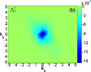
Figure 19: (Color online) Maps of the time-averaged (a) energy-injecting stress, ${\cal H}_{k}$, and nonlinear transfer terms, (b) ${\cal N}_{x}$ and (c) ${\cal N}_{y}$ in k-space for the aspect ratio $(3,2)$. Shown are slices in $(k_{x},k_{y})$-plane at $k_{z}=1$.

Figure 20: Same as in Fig. 15, but for the aspect ratio $(1,2)$. The basic mode corresponds to the maximum energy only during largest bursts, while at other times maximum energy is achieved by other nearby symmetric active modes [bigger black dots in Figs. 21(a) and 21(b)]. The volume-averaged energy follows the maximum spectral energy and therefore the highest peaks are manifestation of the basic mode dynamics (growth) at these times.

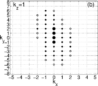
Figure 21: Distribution of the dominant energy-carrying modes in k-space at (a) $k_{z}=0$, (b) $k_{z}=1$ and (c) $k_{z}=2$ for the aspect ratio $(1,2)$. The symbols have the same meaning as in Fig. 16. The most active modes that contribute to the maximum of the spectral energy at least once during the evolution are only symmetric ones, including the basic mode at $k_{x}=k_{y}=0,k_{z}=1$.

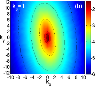
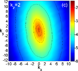
Figure 22: (Color online) Logarithm of the time-averaged kinetic energy spectrum, $log_{10}({\cal E}_{k})$ for the aspect ratio $(1,2)$. The slices in $(k_{x},k_{y})$-plane at (a) $k_{z}=0$, (b) $k_{z}=1$ and (c) $k_{z}=2$ are presented.

Figure 23: Same as in Fig. 18, but for the aspect ratio $(1,2)$. Both the energy and stress achieve their maximum again at $k_{z}=\pm 1$.

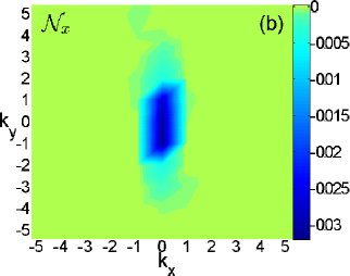
Figure 24: (Color online) Maps of the time-averaged (a) energy-injecting stress ${\cal H}_{k}$, and nonlinear transfer terms, (b) ${\cal N}_{x}$ and (c) ${\cal N}_{y}$ in k-space for the aspect ratio $(1,2)$. Shown are sections of these quantities in $(k_{x},k_{y})$-plane at $k_{z}=1$.

Figure 19 shows the time-averaged stress and the nonlinear transfer functions in spectral space at slices $k_{z}=1$: (a) ${\cal H}_{k}$, (b) ${\cal N}_{x}$ and (c) ${\cal N}_{y}$. Note that all these spectra exhibit qualitatively a similar shape and anisotropy as are in the cubic box. The maximum of the time-averaged stress comes again at the basic mode with ${\bf k}_{b}=(0,0,\pm 1)$, indicating that in time-average sense it is dominant, however, as mentioned above, the basic mode in fact prevails over other modes only during the high burst events [Fig. 15(b)]. The nonlinear transfer term ${\cal N}_{x}$, is negative in the vital area and therefore acts as a sink for streamwise energy there, but transfers it to intermediate and larger wavenumbers where this term is positive. For these modes lying outside the vital area, the stress is negligible and therefore they get energy mainly due to the nonlinear transfer by ${\cal N}_{x}$ rather than from the flow. On the other hand, ${\cal N}_{y}$ exhibits a noticeable dependence on the wavevector angle (i.e., the transverse cascade): ${\cal N}_{y}$ is positive in the first and third quadrants [$k_{y}/k_{x}>0$, yellow and red areas in Fig. 19(c)], where it creates the shearwise velocity, like that in the the cubic box [see Fig. 8(h)]. It is then further amplified jointly by ${\cal N}_{y}$ and the linear shear-induced term on the rhs of Eq. (17), which is also positive in this region of spectral space. The shearwise velocity, undergoing amplification, induces growth of streamwise velocity due to the nonnormality and ultimately stress. As a result, as seen from Fig. 19(a), majority of the stress occurs just in this quadrants of spectral space (at a given $k_{z}$). So, a basic self-sustaining scheme discussed above in the case of the cubic box, extends naturally to this aspect ratio.

Finally, we note that the main distinction between the spectral dynamics of turbulence in the cubic and $(A_{xz},A_{yz})=(3,2)$ boxes is the difference between the number of active, energy-carrying modes and, consequently, the size of the vital area in spectral space. Increasing $A_{xz}$ with respect to $A_{yz}$ introduces more active symmetric and non-symmetric modes into the turbulence dynamics, widening the vital area. Together with the basic mode, more active harmonics with $|k_{z}|=1$ and $k_{z}=0$ reach the maximum spectral energy in succession in short time intervals. Due to this the bursts in the volume-averaged energy evolution are not as pronounced, or strong as for the cubic box, however, largest peaks can still be attributed to the dynamics of the basic mode.

III.3 Aspect ratio $(A_{xz},A_{yz})=(1,2)$

Evolution of the volume-averaged energy in the case of the aspect ratio $(1,2)$ is shown in Fig. 20. In this figure, we also show the time-evolution of the maximum value of the spectral energy and the energy of the basic mode. Note that the volume-averaged energy well follows the maximum spectral energy: the bursts (peaks) in the maximum spectral energy are related to the basic mode dynamics (amplification). Figure 21 displays the active modes (black dots) during the evolution that form the self-sustaining dynamics of turbulence for this aspect ratio. Their total number is 86, more than that in the cubic box but less than that for the aspect ratio $(3,2)$. The vital area, where these modes lie, spans the range $|k_{x}|\leq 2,|k_{y}|\leq 7,|k_{z}|\leq 2$. Note that compared to the cubic box (Fig. 5), increasing $A_{yz}$ with respect to $A_{xz}$ introduces more active modes with larger $k_{y}$, but with the same $k_{x}$ and $k_{z}$, resulting in the extension of the vital area along the $k_{y}$-axis. Together with the basic mode with ${\bf k}_{b}=(0,0,\pm 1)$, the five symmetric modes – two with $k_{z}=0$ and three with $k_{z}=1$ [shown with bigger black dots in Figs. 21(a) and 21(b)], contribute to the maximum spectral energy, ${\cal E}_{k,max}$. As a result, the peaks in the volume-averaged energy appear more pronounced than that in the case $(3,2)$, where larger number of modes reach comparable energy maxima. However, as evident from Fig. 20(b), during the largest bursts, the maximum of the spectral energy is still due to the basic mode, as in the case of the above two aspect ratios. So, the conclusion drawn above that the stronger bursts in the total energy are associated with the basic mode dynamics holds also for the aspect ratio $(1,2)$.

The time-averaged energy spectrum at three different $k_{z}=0,1,2$ is shown in Fig. 22. It exhibits the same type of anisotropy due to shear as those in the above two cases. The time-averaged energy and stress spectra integrated in $(k_{x},k_{y})$-plane is represented as a function of $k_{z}$ in Fig. 23. Both spectra reach maximum again at $k_{z}=\pm 1$ and decrease with $|k_{z}|$. Compared to the aspect ratio $(3,2)$, at $k_{z}=0$, the integrated spectral energy is smaller than that at $k_{z}=\pm 1$ and the integrated stress is again small, implying that a net energy extraction by 2D modes is much less effective compared to that by 3D modes. Figure 24 shows the time-averaged spectra of the stress and nonlinear transfer functions at $k_{z}=1$, which are qualitatively similar to those for the other two aspect ratios considered above and hence the self-sustaining process works in the same way.

IV summary and discussion

We considered a spectrally stable flow with constant shear of velocity, where the only energy supply of (subcritical) turbulence is due to the flow nonnormality-induced linear growth of perturbations. To understand the underlying self-sustenance mechanism of homogeneous turbulence in this flow, we performed DNS and analyzed the dynamical processes in Fourier space. From the Navier-Stokes equations we derived the evolution equations for the perturbed velocity components in wavenumber space using Fourier transformation. We explicitly calculated and visualized individual linear and nonlinear terms in these spectral equations and analyzed them in detail qualitatively as well as quantitatively based on the DNS data.

The main results corresponding to the five objectives outlined in Introduction are summarized below:

– We first calculated the dynamically important optimal harmonics (Fig. 1) using the linear nonmodal analysis and identified the range of aspect ratios, $A_{xz}\leq A_{yz}$ and $A_{xz}\geq 1$, for which as many of them as possible are included in the simulation domain. Afterwards, based on this, we considered three aspect ratios of the flow domain: cubic $(A_{xz},A_{yz})=(1,1)$, streamwise elongated $(A_{xz},A_{yz})=(3,2)$ and shearwise elongated $(A_{xz},A_{yz})=(1,2)$ boxes to understand the dependence of the turbulence dynamics on the latter.

– The Reynolds stress, which is of linear origin, is responsible for the energy extraction from the flow into turbulence via the nonmodal growth of Fourier harmonics of perturbations. In the nonlinear regime, we identified a range of wavenumbers in which this growth is significant and hence the dynamically active modes that determine the self-sustenance process of the turbulence, carrying high values of energy and Reynolds stress (Figs. 5, 16, 21). They have length scales comparable to the box size and hence are mainly concentrated at small wavenumbers in Fourier space, which is suitably labeled as the vital area of the turbulence.

– From these active harmonics, those contributing to the maximum of the spectral energy and stress play a key role in the self-sustenance process (bigger black dots in Figs. 5, 16, 21). They have smallest spanwise wavenumbers $k_{z}=0,2\pi/L_{z}$ and their number generally depends on the box aspect ratio. It was shown that for all the three aspect ratios considered, the basic large scale mode with the wavenumber ${\bf k}_{b}=(0,0,\pm 2\pi/L_{z})$ plays a special role in the homogeneous shear turbulence dynamics, consistent with previous study by Pumir Pumir (1996). For the cubic box, it is the only mode that yields the maximum spectral energy and Reynolds stress in Fourier space during the entire evolution, much larger than that of the nearby active modes, and undergoes the largest nonmodal amplification. This amplification occurs in bursts, alternating with decaying intervals (Fig. 2). During these bursts, it contributes up to $70\%$ of the total Reynolds stress. As a result, the basic mode is responsible for the production of a major fraction of the turbulence’s total energy and largely determines its behavior – the total energy also exhibits bursts closely following those of the basic mode. Such bursting events in the energy are also observed in turbulent boundary layers Robinson (1991); Jiménez et al. (2005) and the homogeneous shear turbulence model is often invoked to understand their nature Pumir (1996); Sekimoto et al. (2016). The prevalence of the basic mode is somewhat reduced for other two aspect ratios. We found that increasing streamwise or/and shearwise dimensions of the box introduces more modes, respectively, along these directions in the vital area, which grow comparably with the basic mode, also corresponding to the maximum of the spectral energy at certain times during evolution. As a result, their contribution to the total energy increases. The evolution of the latter is now determined by these active modes, rather than by the basic mode only. Due to this, the total energy is characterized by weaker bursts, especially for the aspect ratio $(A_{xz},A_{yz})=(3,2)$, with the largest number of the active modes in the vital area. Nevertheless, the appearance of highest bursts in the total energy and stress appears to be related to the basic mode dynamics for these aspect ratios too (Figs. 15, 20).

– The nonmodal growth process and, therefore the resulting energy and Reynolds stress spectra, are anisotropic in Fourier ($\bf k$-) space, i.e., mainly depend on the orientation of wavevector (Figs. 8, 19, 24). This anisotropy of the linear processes in shear flows, in turn, leads to anisotropy of nonlinear processes in Fourier space: the nonlinear terms, which do not directly draw the background flow energy, transversely redistribute this energy over wavevector angles. It was found that this new – transversal – type of nonlinear redistribution of harmonics, referred to as the transverse cascade, is a generic feature of nonlinear dynamics of perturbations in spectrally stable shear flows. It differs from and represents an alternative to the classical energy cascade processes (direct/inverse) in shear flow turbulence. Previously, the transverse cascade was also demonstrated to take place and play an important role in 2D HD and MHD shear flows Horton et al. (2010); Mamatsashvili et al. (2014). This cooperation of anisotropic linear and nonlinear processes, in turn, gives rise to an anisotropic energy spectrum in shear flows, which, in general, differs from the classical Kolmogorov spectrum in homogeneous turbulence without background shear, especially at small and intermediate wavenumbers. As a result, the transverse cascade may naturally appear to be a keystone of the bypass concept of subcritical turbulence in spectrally stable HD shear flows, which is being actively discussed among the hydrodynamical community. Therefore, the conventional description of shear flow turbulence solely in terms of direct and inverse cascades, which leaves out the transverse cascade, might be incomplete and misleading.

– The vital area in wavenumber space is the primary site of activity of the energy-supplying linear nonmodal growth and the nonlinear transverse cascade that lie at the heart of the self-sustaining dynamics of turbulence. The course of events ensuring the self-sustenance of the turbulence is as follows. The transverse cascade continually transfers harmonics to those quadrants of the vital area where the shear flow causes linear nonmodal growth, i.e., regenerates harmonics that can undergo amplification due to the flow nonnormality, and thereby closes feedback loop ensuring sustenance of the turbulence. This general picture comprises refined, somewhat differing interplay of linear and nonlinear processes for the basic mode and active symmetric and non-symmetric modes. These, qualitatively quite simple but quantitatively a bit involved schemes are described in detail for different aspect ratios in Section III (see also Figs. 10-14). Thus, we have demonstrated that in the considered constant shear flow, the turbulence is maintained by a subtle interplay between linear and nonlinear processes: the first supplies energy for turbulence via shear-induced nonmodal growth process (characterized by the Reynolds stresses) and the second plays an important role of providing a positive feedback that makes this growth process long-lived against viscous dissipation, which would otherwise be transient in the absence of the latter.

The number of the active harmonics (defined as the harmonics whose energies grow more than $10\%$ of the maximum spectral energy at least once during the evolution) in the vital area, which are the main participants in the turbulence dynamics, generally depends on the box aspect ratio and is quite large. In the considered here aspect ratios, it exceeds 35 for the cubic box and can be more than 200 for longer boxes in the streamwise or shearwise directions (see Figs. 5, 16 and 21), indicating fairly complex nature of self-sustaining dynamics of turbulence, which apparently cannot be described by low-order models. In this paper, performing a full DNS, the realization of the nonlinear transverse cascade and its role in the self-sustenance of homogeneous shear turbulence are demonstrated in the most general manner, without truncating the number of modes and using other simplifying assumptions usually made in low-order models of self-sustaining processes (e.g., Refs. Waleffe (1995, 1997); Moehlis et al. (2004)). Nevertheless, one can relate the described here self-sustaining scheme of homogeneous shear turbulence in the constant shear flow without (physical) boundaries to the self-sustenance scenario in low-order models which, however, commonly include walls affecting the dynamics (see e.g., Refs. Farrell and Ioannou (2012); Thomas et al. (2014, 2015)). Namely, the nonlinear regeneration of streamwise rolls is analogous to the production of shearwise velocity due to the nonlinear transfer terms and the generation and nonmodal amplification of streamwise streaks from the former due to shear (nonnormality) is similar to the amplification of streamwise velocity. One of the main results of the present study is that the self-sustaining process of turbulence in spectrally stable shear flows in fact does not require the presence of walls and is intrinsic to the flow system itself, being governed by the interplay between linear nonnormality-induced and the nonlinear transverse cascade processes.

Finally, we would like to emphasize that revealing the new aspects of the homogeneous shear turbulence dynamics – anisotropic energy spectra, the nonlinear transverse cascade and the notion of the vital area, where the self-sustaining process is concentrated, have become largely possible owing to analysis in Fourier space. This allows us to gain a deeper insight into turbulence dynamics and its underlying sustenance mechanism. At the same time, the performed simulations show that the basic mode, which is central in the energy exchange between the shear flow and turbulence, has a large scale spanwise variation and is uniform in the streamwise and shearwise directions, $k_{x}=k_{y}=0,k_{z}=\pm 2\pi/L_{z}$; it has streamwise and shearwise velocities, but zero spanwise velocity. This simple configuration (geometry) of the basic mode makes it easily describable in physical space too – its amplification due to the nonnormality can be readily understood from Eqs. (3) and (4) in physical space. The streamwise velocity $u_{x}$ is generated from the shearwise velocity due to shear (linear term -$Su_{y}$ in Eq. 3). As a result, this two velocities correlate and produce positive stress, extracting flow energy. The role of nonlinearity in Eq. (4) is then to regenerate the shearwise velocity $u_{y}$.

Appendix A Fourier transform in the presence of shear

As discussed in the text, $k_{y}$ of an individual harmonic linearly changes with time, $k_{y}(t)=k_{y}(0)-Sk_{x}t$, due to the background shear flow, that is also consistent with the shear-periodic boundary conditions (see e.g., Refs. Farrell (1987); Chagelishvili et al. (2003); Jiménez (2013)). For this reason, a standard FFT technique cannot be applied for calculating Fourier transforms along this direction during post-processing. To circumvent this problem, we used the approach of Refs. Mamatsashvili and Rice (2009); Heinemann and Papaloizou (2009), which we recap below.

In a finite computational domain, streamwise $k_{x}$ and spanwise $k_{z}$ wavenumbers are both discrete: $k_{x}=2\pi n_{x}/L_{x},k_{z}=2\pi n_{z}/L_{z}$, while the shearwise wavenumber is $k_{y}(t)=2\pi n_{y}/L_{y}-St(2\pi n_{x}/L_{x})$, where $n_{x},n_{y},n_{z}$ are integers, $-N_{x}/2\leq n_{x}\leq N_{x}/2,-N_{y}/2\leq n_{y}\leq N_{y}/2,-N_{z}/2\leq n_{z}\leq N_{z}/2$. In this case, any flow field at time $t$ can be decomposed in Fourier expansion

$$f(x,y,z,t)=\sum_{n_{x},n_{y},n_{z}}\bar{f}_{n_{x},n_{y},n_{z}}(t){\rm exp}[{\rm i}k_{x}x+{\rm i}k_{y}(t)y+{\rm i}k_{z}z],$$

where the Fourier coefficients can be computed from the inverse transform

$$\bar{f}_{n_{x},n_{y},n_{z}}(t)=\frac{1}{L_{x}L_{y}L_{z}}\times\\ \int\int\int f(x,y,z,t){\rm exp}[-{\rm i}k_{x}x-{\rm i}k_{y}(t)y-{\rm i}k_{z}z]dxdydz,$$

or more explicitly, after separating out the time-dependent part in the exponent and rearranging, we get

$$\bar{f}_{n_{x},n_{y},n_{z}}(t)=\\ \frac{1}{L_{y}}\int{\rm exp}\left({\rm i}St\frac{2\pi n_{x}}{L_{x}}y\right)\left[\frac{1}{L_{x}L_{z}}\int\int f(x,y,z,t)\times\right.\\ \left.{\rm exp}\left(-{\rm i}\frac{2\pi n_{x}}{L_{x}}x-{\rm i}\frac{2\pi n_{z}}{L_{z}}z\right)dxdz\right]{\rm exp}\left(-{\rm i}\frac{2\pi n_{y}}{L_{y}}y\right)dy.$$

This last expression suggest the way to compute the Fourier transform of a real quantity from the simulation in the presence of shear. So, we first do a standard FFT in $x$- and $z$-directions, multiply the result by ${\rm exp}[{\rm i}St(2\pi n_{x}/L_{x})y]$, which accounts for the effect of shear, and finally do again FFT in the $y$-direction. The time-dependent shearwise wavenumber associated with the Fourier coefficient $\bar{f}_{n_{x},n_{y},n_{z}}$ at time $t$ is given by

$$k_{y}(t)=\frac{2\pi n_{y}}{L_{y}}-St\frac{2\pi n_{x}}{L_{x}}+l\frac{2\pi N_{y}}{L_{y}},$$

where an integer number $l$ is chosen such that to ensure $k_{y}(t)$ always stays within the numerical domain in spectral space

$$-\frac{\pi L_{y}}{N_{y}}\leq k_{y}(t)\leq\frac{\pi L_{y}}{N_{y}}.$$

References

- Farrell (1988) B. F. Farrell, Phys. Fluids 31, 2093 (1988).
- Butler and Farrell (1992) K. M. Butler and B. F. Farrell, Phys. Fluids 4, 1637 (1992).
- Reddy et al. (1993) S. Reddy, P. Schmid, and D. Henningson, SIAM J. Appl. Math. 53, 15 (1993).
- Trefethen et al. (1993) L. N. Trefethen, A. E. Trefethen, S. C. Reddy, and T. A. Driscoll, Science 261, 578 (1993).
- Reddy and Henningson (1993) S. C. Reddy and D. S. Henningson, J. Fluid Mech 252, 209 (1993).
- Schmid and Henningson (2001) P. J. Schmid and D. S. Henningson, Stability and Transition in Shear Flows (Springer, 2001).
- Criminale et al. (2003) W. O. Criminale, T. L. Jackson, and R. D. Joslin, Theory and Computation of Hydrodynamic Stability, by W. O. Criminale and T. L. Jackson and R. D. Joslin, pp. 464. Cambridge, UK: Cambridge University Press. (2003).
- Schmid (2007) P. J. Schmid, Annu. Rev. Fluid Mech. 39, 129 (2007).
- Zhuravlev and Razdoburdin (2014) V. V. Zhuravlev and D. N. Razdoburdin, Mont. Not. R. Astron. Soc. 442, 870 (2014).
- Farrell and Ioannou (1994) B. F. Farrell and P. J. Ioannou, Phys. Rev. Lett. 72, 1188 (1994).
- Gebhardt and Grossmann (1994) T. Gebhardt and S. Grossmann, Phys. Rev. E 50, 3705 (1994).
- Henningson and Reddy (1994) D. S. Henningson and S. C. Reddy, Phys. Fluids 6, 1396 (1994).
- Baggett et al. (1995) J. S. Baggett, T. A. Driscoll, and L. N. Trefethen, Phys. Fluids 7, 833 (1995).
- Grossmann (2000) S. Grossmann, Rev. Mod. Phys. 72, 603 (2000).
- Chapman (2002) S. J. Chapman, J. Fluid Mech. 451, 35 (2002).
- Eckhardt et al. (2007) B. Eckhardt, T. M. Schneider, B. Hof, and J. Westerweel, Annu. Rev. Fluid Mech. 39, 447 (2007).
- Farrell and Ioannou (2012) B. F. Farrell and P. J. Ioannou, J. Fluid Mech. 708, 149 (2012).
- Brandt (2014) L. Brandt, Eur. J. Mech. B-Fluid. 47, 80 (2014).
- Tavoularis and Corrsin (1981) S. Tavoularis and S. Corrsin, J. Fluid Mech. 104, 311 (1981).
- Rogers and Moin (1987) M. M. Rogers and P. Moin, J. Fluid Mech. 176, 33 (1987).
- Lee et al. (1990) M. J. Lee, J. Kim, and P. Moin, J. Fluid Mech. 216, 561 (1990).
- Kida and Tanaka (1994) S. Kida and M. Tanaka, J. Fluid Mech. 274, 43 (1994).
- Pumir and Shraiman (1995) A. Pumir and B. Shraiman, Phys. Rev. Lett. 75, 3114 (1995).
- Waleffe (1995) F. Waleffe, Phys. Fluids 7, 3060 (1995).
- Waleffe (1997) F. Waleffe, Phys. Fluids 9, 883 (1997).
- Pumir (1996) A. Pumir, Phys. Fluids 8, 3112 (1996).
- Sekimoto et al. (2016) A. Sekimoto, S. Dong, and J. Jiménez, Phys. Fluids 28, 035101 (2016).
- Farrell (1987) B. Farrell, J. Atmos. Sci. 44, 2191 (1987).
- Farrell and Ioannou (1993) B. F. Farrell and P. J. Ioannou, Phys. Fluids 5, 1390 (1993).
- Jiménez (2013) J. Jiménez, Phys. Fluids 25, 110814 (2013).
- Chagelishvili et al. (2002) G. D. Chagelishvili, R. G. Chanishvili, T. S. Hristov, and J. G. Lominadze, Sov. Phys. JETP 94, 434 (2002).
- Horton et al. (2010) W. Horton, J.-H. Kim, G. D. Chagelishvili, J. C. Bowman, and J. G. Lominadze, Phys. Rev. E 81, 066304 (2010).
- Mamatsashvili et al. (2014) G. Mamatsashvili, G. Gogichaishvili, G. Chagelishvili, and W. Horton, Phys. Rev. E 89, 043101 (2014).
- Salhi et al. (2014) A. Salhi, F. G. Jacobitz, K. Schneider, and C. Cambon, Phys. Rev. E 89, 013020 (2014).
- Chagelishvili et al. (2003) G. D. Chagelishvili, J.-P. Zahn, A. G. Tevzadze, and J. G. Lominadze, Astron. Astrophys. 402, 401 (2003).
- Tevzadze et al. (2003) A. G. Tevzadze, G. D. Chagelishvili, J.-P. Zahn, R. G. Chanishvili, and J. G. Lominadze, Astron. Astrophys. 407, 779 (2003).
- Umurhan and Regev (2004) O. Umurhan and O. Regev, Astron. Astrophys. 427, 855 (2004).
- Rempfer (2003) D. Rempfer, Annu. Rev. Fluid Mech. 35, 229 (2003).
- Kim et al. (1987) J. Kim, P. Moin, and R. Moser, J. Fluid Mech. 177, 133 (1987).
- Lele (1992) S. K. Lele, J. Comput. Phys. 103, 16 (1992).
- Rogallo (1981) R. Rogallo, Numerical experiments in homogeneous turbulence, TechReport (NASA, 1981).
- Mamatsashvili and Rice (2009) G. R. Mamatsashvili and W. K. M. Rice, Mon. Not. R. Astro. Soc. 394, 2153 (2009).
- Heinemann and Papaloizou (2009) T. Heinemann and J. C. B. Papaloizou, Mon. Not. R. Astron. Soc. 397, 64 (2009).
- Farrell and Ioannou (1996) B. F. Farrell and P. J. Ioannou, J. Atmos. Sci. 53, 2025 (1996).
- Biskamp (2003) D. Biskamp, Magnetohydrodynamic turbulence (Cambridge University Press, 2003).
- Note (1) Although of every harmonic with changes with time as a result of drift due to shear flow, we can still take Eulerian approach and focus on a fixed in spectral space.
- Note (2) The correlation coefficient between two time-dependent functions and is defined in a usual way as Pearson’s product-moment correlation coefficient. The time average is done over an entire duration of the saturated turbulent state in the simulations.
- Robinson (1991) S. K. Robinson, Ann. Rev. Fluid Mech. 23, 601 (1991).
- Jiménez et al. (2005) J. Jiménez, G. Kawahara, M. P. Simens, M. Nagata, and M. Shiba, Phys. Fluids 17, 015105 (2005).
- Moehlis et al. (2004) J. Moehlis, H. Faisst, and B. Eckhardt, New J. Phys. 6, 56 (2004).
- Thomas et al. (2014) V. L. Thomas, B. K. Lieu, M. R. Jovanović, B. F. Farrell, P. J. Ioannou, and D. F. Gayme, Phys. Fluids 26, 105112 (2014).
- Thomas et al. (2015) V. L. Thomas, B. F. Farrell, P. J. Ioannou, and D. F. Gayme, Phys. Fluids 27, 105104 (2015).