Mutually cooperative epidemics on power-law networks

Abstract

The spread of an infectious disease can, in some cases, promote the propagation of other pathogens favouring violent outbreaks, which cause a discontinuous transition to an endemic state. The topology of the contact network plays a crucial role in these cooperative dynamics. We consider a susceptible–infected–removed (SIR) type model with two mutually cooperative pathogens: an individual already infected with one disease has an increased probability of getting infected by the other. We present an heterogeneous mean-field theoretical approach to the co–infection dynamics on generic uncorrelated power-law degree-distributed networks and validate its results by means of numerical simulations. We show that, when the second moment of the degree distribution is finite, the epidemic transition is continuous for low cooperativity, while it is discontinuous when cooperativity is sufficiently high. For scale-free networks, i.e. topologies with diverging second moment, the transition is instead always continuous. In this way we clarify the effect of heterogeneity and system size on the nature of the transition and we validate the physical interpretation about the origin of the discontinuity.

I Introduction

Modelling epidemic dynamics plays a key role in predicting disease outbreaks and designing effective strategies to prevent or control them. While traditional theories of disease propagation ignore network effects, there has been a large amount of research in the past decades aimed at understanding how the topological structure of contact networks affects the dynamics upon them Pastor-Satorras et al. (2015). Such studies have focused mainly on the dynamics of a single epidemic disease.

An issue of growing interest in current epidemiological research is how concurrent spreading diseases interact with each other. Such coupled spreading scenarios can occur when either multiple pathogens or multiple strains of the same disease simultaneously propagate in the same population. The complexity of the problem is largely increased already in the two–pathogen case. Two diseases circulating in the same host population can interact in many different ways, with either synergistic or antagonistic effects.

A well known type of interaction is cross–immunity: an individual infected with one disease becomes partially or fully immune to infection by the second one. In this case the two pathogens compete for the same population of hosts. The competition between epidemics that are mutually exclusive or antagonistic was studied in Newman (2005a); Funk and Jansen (2010); Marceau et al. (2011); Miller (2013).

An opposite case that is recently gaining attention is the spreading of two or more cooperating pathogens: in this case an individual that is already infected with one disease has increased chance of getting infected with another. A notable example is the 1918 Spanish flu pandemic that involved about one–third of the world’s population killing tens of millions of people within months  Taubenberger and Morens (2006). A considerable proportion of the infected were co–infected by pneumonia Morens et al. (2008); Brundage and Shanks (2008), and most deaths where caused not directly by the virus, but by the secondary bacterial infection. Another well–known case is that of HIV, which increases the host susceptibility to other pathogens, in particular to the hepatitis C virus (HCV) Sulkowski (2008).

In co–infections, positive feedback between multiple diseases can lead to more rapid outbreaks. One of the most interesting questions is whether cooperation can change the epidemic transition from being continuous to abrupt when external conditions vary, even slightly, as for a microscopic change in infectivity. This is an extremely relevant problem since the possibility to enact countermeasures critically depends on the type of transition: in the discontinuous case the epidemic can take over a population explosively without any of the warning signs which occur in single epidemics.

Recently Newman and Ferrario (2013) Newman and Ferrario introduced a model of co-infection based on the susceptible–infected–removed (SIR) model Kermack and McKendrick (1927) with two diseases diffusing over the same contact network. One disease spreads freely while the second can only infect individuals already infected with the first. The authors assume total asymmetry and time–scale separation in the spreading of the two pathogens. The system displays two epidemic thresholds, the first one being the usual SIR threshold, the second occurring when the fraction of the population infected with the first disease becomes large enough to allow the spread of the second. No qualitative changes in the nature of the outbreaks appear. In Chen et al. (2013) Chen, Ghanbarnejad, Cai, and Grassberger (CGCG) introduced a generalized SIR model (CGCG model) to include mutual cooperative effects of co–infections. In the CGCG model two different diseases simultaneously spread in a population. Having being infected with one disease gives an increased probability to get infected by the other. The amount of this increase is a proxy of the mutual cooperativity between the two diseases. The authors study the model at mean–field level and observe that cooperative effects, depending of their strength, can cause a change of the transition from continuous to discontinuous. In Janssen and Stenull (2016) Janssen and Stenull showed that the CGCG model is equivalent, in mean–field, to the homogeneous limit of an extended general epidemic process and clarify the spinodal nature of the discontinuous transition observed. In Cai et al. (2015); Grassberger et al. (2016) CGCG analyzed how in their model the type of transition depends on the contact network topology by simulating the CGCG model on both random networks and lattices. They concluded that a necessary condition for discontinuous transitions to occur, when starting from a doubly-infected node, is the relative paucity of short loops with respect to long ones. More in detail they argue that a discontinuous transition occurs if the two epidemics first evolve separately and, only after the independent clusters of singly-infected nodes have reached endemic proportions, the two epidemics meet: at that point cooperativity implies that both clusters rapidly become doubly infected. A necessary condition then is that there are few short loops (otherwise the two pathogens immediately cooperate and the transition is continuous) and there are long loops (otherwise cooperativity has no effect and one sees only single infections). In agreement with this scenario CGCG do not observe discontinuous transitions on trees and on 2–d lattices, while they do observe them on Erdös–Rényi (ER) networks, on 4–d lattices, and on 2–d lattices with sufficiently long-range contacts. On 3–d lattices the existence of discontinuous transitions depends on the details of the microscopic realization of the model. Moreover, the observed discontinuous transitions are of hybrid type Goltsev et al. (2006); Parisi and Rizzo (2008), i.e., exhibiting also some features of continuous ones. For other recent work about cooperating infections see Refs. Sanz et al. (2014); Azimi-Tafreshi (2016); Chen et al. (2016).

An open question left by the analysis in Cai et al. (2015); Grassberger et al. (2016) has to do with what happens for co–infections on generic broadly degree-distributed networks. Simulations performed on a Barabasi–Albert (BA) topology seem to indicate a continuous transition even for strong cooperativity. However, it is not clear whether these results are affected by finite size effects and what happens for co–infections on other broadly distributed networks. Theoretical approaches Chen et al. (2013); Janssen and Stenull (2016) deal only with homogeneous networks.

In this paper we elucidate these issues. We first numerically show that for power-law distributed networks of large size the transition is asymptotically discontinuous, if cooperativity is sufficiently high; however strong size effects may conceal the real nature of the transition in finite systems, so that the transition appears continuous even for large networks. We then present an analytical heterogeneous mean-field approach to the problem, which allows us to derive a number of predictions, including the position of the threshold, the nature of the transition and the associated critical exponent. Numerical simulations validate the analytical predictions. The theoretical approach indicates that for scale-free networks, with diverging second moment of the degree distribution, the transition can only be continuous.

The paper is organized as follows. In Sec. II we describe the CGCG model in detail. Sec. III is devoted to a numerical investigation of the nature of the transition for power-law degree-distributions, showing how finite size effects can hinder the emergence of the discontinuity in scale-rich networks. Sec. IV is devoted instead to the theoretical analysis of the co-infection dynamics by means of a heterogeneous mean–field approach. Theoretical results are compared with numerical simulations, revealing a satisfactory agreement. We present conclusions and an outlook in Sec. V.

II Model

In the classical SIR model in discrete time, each individual can be in one of three different states: susceptible (S, individuals that are healthy, neither infected nor immune), infected (I, individuals who can transmit the disease), or removed (R, dead or recovered and immunized individuals). At each time step each infected individual spontaneously decays with probability $r$ into the removed state, while she transmits the infection to each of her susceptible neighbors with probability $p$.

The CGCG model is a modification of the SIR model with two circulating diseases, A and B. The infection probability for one disease is increased if the individual currently has, or has had in the past, the other disease: Individuals uninfected by either disease get infected (with either A or B) by any infective neighbour with probability $p$, while a node that is or has been infected by one disease has a higher probability $q>p$ to get infected by the other pathogen. When recovering from one disease an individual becomes immune to that disease, but she can still be infected by the other. The model is totally symmetric with respect to A and B. Since each individual can be in one of three possible states (S, I, R) with respect to each of the two diseases (A, B) there are nine possible states for each individual, denoted by S, A, B, AB, a, b, aB, Ab and ab, where, for each disease, capital letters refer to the infected state, while lower–case letters refer to the removed state. States denoted by single letters (a, b, A, B) refer to states where the individual is still susceptible with respect to the other disease.

We simulate the CGCG model on power-law distributed networks $P(k)\sim k^{-\gamma}$, generated according to the uncorrelated configuration model Catanzaro et al. (2005), for various values of the $\gamma$ exponent. We fix the recovery probability to $r=1$ throughout the paper. In the various simulations, a number $N_{r}$ (ranging from 200 to 2000) of independent realizations are performed. We consider an initial condition with all individuals initially in the susceptible (S) state except for a single, randomly chosen individual who is in the doubly-infected AB state.

III Finite size effects and the nature of the transition for high cooperativity

We start by analyzing the behavior of the CGCG model on power-law degree-distributed networks. In Ref. Cai et al. (2015) only continuous transitions were observed for the Barabasi–Albert (BA) scale–free network. This is in contrast with the behavior of the same model on Erdös–Rényi networks, which exhibits a discontinuous transition for sufficiently high cooperativity. One may wonder whether the continuity of the transition for BA networks persists in the infinite size limit and whether the same occurs for other broadly distributed networks, which are however not scale-free.

The interpretation for the existence of a discontinuous transition put forward in Ref. Cai et al. (2015) provides some hint on the issue. The origin of the discontinuity is traced back to the relative abundance of long loops compared to the scarcity of short loops in the topology. It is well known Newman (2005b) that the clustering coefficient of uncorrelated random networks is

$$C=\frac{\left\langle{k}\right\rangle}{N}\left(\frac{\left\langle{k^{2}}\right\rangle-\left\langle{k}\right\rangle}{\left\langle{k}\right\rangle^{2}}\right)^{2}.$$ (1)

Hence the clustering coefficient vanishes for large size for any $\gamma>2$. However, this occurs differently depending on the value of $\gamma$. The factor in parentheses in Eq. (1) is finite for $\gamma>3$, but its value becomes larger as $\gamma$ gets smaller. Hence we do expect that for systems of fixed size $N$ the transition will be discontinuous for large $\gamma$, but the residual clustering will make the transition appear continuous as $\gamma$ is reduced. This expectation is tested by simulating the CGCG dynamics on networks of fixed size ($N=10^{5}$), large cooperativity ($q=0.99$) and growing values of $\gamma$ starting from $\gamma=3$ (Fig. 1).

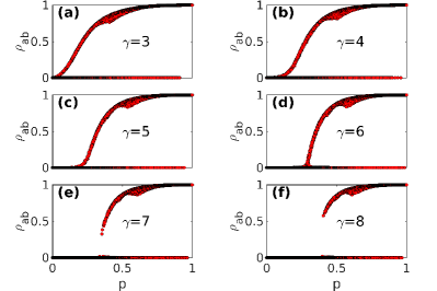
FIG. 1: The six panels represent the total density $\rho_{ab}$ of population recovered from both A and B in the final state plotted versus $p$ on scale–free networks with $\gamma=3,4,5,6,7,8$, built by applying the uncorrelated configuration model. The system size is $N=10^{5}$, and $q=0.99$. The results are averaged over a number $N_{r}$ of independent realizations that is $200$ for $\gamma=3$ to 5 and is increased to $2000$ for $\gamma=6$ to 8.

As expected, upon increasing $\gamma$, the transition becomes discontinuous: short loops become less abundant as $\gamma$ grows so that the two infections evolve separately and give rise to cooperative effects only after they meet following one long loop in the network.

Further evidence about the same effect is obtained by simulating the CGCG dynamics on a network with fixed $\gamma=7$ and increasing system size from $N=10^{3}$ to $10^{6}$ (see Fig. 2): when the size is big enough the discontinuity appears.

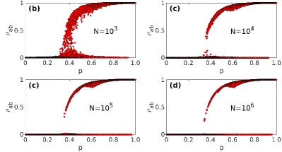
FIG. 2: Total density $\rho_{ab}$ of population recovered from both A and B in the final state, plotted versus $p$ on scale–free networks of different sizes ($N=10^{3},10^{4},10^{5},10^{6}$, respectively), with $\gamma=7$. The parameter $q$ is $0.99$. The results are averaged over $N_{r}=200,500,2000,2000$ independent realizations in panels a,b,c,d, respectively.

The transition presented in Fig. 2 is discontinuous but Fig. 3 shows that it is in fact of hybrid type, as discussed in Ref. Cai et al. (2015). This means that already at the transition point there may be giant infected clusters occupying a finite fraction of the system (see Fig. 3(a) and  3(c)); this is at odds with what happens in the usual, continuous, percolation transition. However the probability that one of these clusters appears undergoes a continuous transition at the threshold (Fig. 3(b)) as in normal percolation.

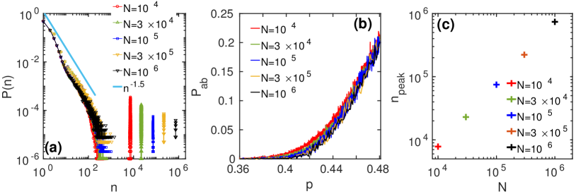
FIG. 3: (a) Mass distribution of doubly-infected clusters at the threshold $p_{c}=\left\langle{k}\right\rangle/(\left\langle{k^{2}}\right\rangle-\left\langle{k}\right\rangle)=0.43388$. The number of realizations is at least $N_{r}=10^{5}$ and various values of $N$. (b) Probability $P_{ab}$ of forming a giant cluster (with size larger than $0.05N$) as a function of $p$ and system sizes ranging (top to bottom) from $N=10^{4}$ to $N=10^{6}$. The number of realizations is $N_{r}=2000$. (c) Plot of the size of the giant cluster as a function of $N$ for $p=p_{c}$, showing a linear growth. All data are for $\gamma=7$ and $q=0.99$.

For values $2<\gamma<3$, Eq. (1) points out that, since $\left\langle{k^{2}}\right\rangle$ diverges as $k_{max}^{2(3-\gamma)}=N^{(3-\gamma)}$, the decay of $C$ with the system size becomes $N^{2-\gamma}$, slower than $1/N$. This qualitative change does not allow to draw firm conclusions on the nature of the transition for $\gamma<3$. Asymptotically the clustering coefficient vanishes also in this case, but it does so slowly so that it might be impossible for the two epidemics to grow initially separated clusters. Therefore we cannot say whether the continuous transition observed in Ref. Cai et al. (2015) is a finite size effect or not. More on this issue will be provided by the analytical results in the next Section.

IV Heterogeneous Mean-Field Theory for uncorrelated networks

In this section we present an analytical approach to the cooperative dynamics on uncorrelated networks, based on the heterogeneous mean-field (HMF) theory Pastor-Satorras and Vespignani (2001); Moreno et al. (2002). It is a refinement of the homogeneous mean-field used in Ref. Chen et al. (2013), that allows for quantities to depend on the degree $k$ of the node considered and is thus suitable also for topologies with a broad connectivity distribution. For example, $[A]_{k}$ is the fraction of individuals in state A, restricted to nodes of degree $k$.

Following the same formalism of Chen et al. (2013), and exploiting the full symmetry among A and B pathogens, we define the quantities

$$Y_{k} = [A]_{k}+[a]_{k}=[B]_{k}+[b]_{k}$$ (2)

$$X_{k} = [A]_{k}+[Ab]_{k}+[AB]_{k}=[B]_{k}+[aB]_{k}+[AB]_{k}$$ (3)

$$R_{k} = [b]_{k}+[bA]_{k}+[ab]_{k}=[a]_{k}+[aB]_{k}+[ab]_{k}\,.$$ (4)

$Y_{k}$ is the fraction of nodes of degree $k$ which have contracted one of the infections and are susceptible with respect to the other; $X_{k}$ is the fraction of nodes of degree $k$ which are currently infected by one of the pathogens, regardless of the state with respect to the other infection; $R_{k}$ is instead the fraction of nodes which have recovered from one infection, regardless of the state with respect to the other. Eqs. (4) of Ref. Chen et al. (2013) can thus be generalized to

$$\dot{S}_{k} =-2\alpha kS_{k}\Theta_{X}$$ (5a)

$$\dot{Y}_{k} =k(\alpha S_{k}-\beta Y_{k})\Theta_{X}$$ (5b)

$$\dot{X}_{k} =k(\alpha S_{k}+\beta Y_{k})\Theta_{X}-\mu X_{k}$$ (5c)

$$\dot{R}_{k} =\mu X_{k}\,,$$ (5d)

which conserve the total probability $S_{k}+Y_{k}+X_{k}+R_{k}=1$. The rates for the transmission of the first infection, of the second infection and for recovery are $\alpha$, $\beta$ and $\mu$, respectively. $\Theta_{X}$ is the probability that any given edge points to an infected node and is capable of transmitting the disease. For SIR dynamics one must take into account the fact that an infected individual cannot transmit the infection through the edge from which she was infected, hence Boguñá et al. (2003)

$$\Theta_{X}=\frac{1}{\left\langle{k}\right\rangle}\sum\limits_{k}(k-1)P(k)X_{k}(t).$$ (6)

In the following we set the recovery rate $\mu=1$, with no loss of generality. Notice that Eqs. (5) are for continuous dynamics, while the dynamics considered in simulations are discrete, with lifetime of the infected state deterministically equal to 1. In order to compare results between theory and simulation, we must therefore consider the mapping between the rates and the probabilities $\alpha=p/(1-p)$ and $\beta=q/(1-q)$ (see Appendix A).

Considering the initial condition with only one doubly-infected node $S_{k}(0)\simeq 1$, $R_{k}(0)=Y_{k}(0)=0$ and $X_{k}(0)=1-S_{k}(0)\simeq 0$, Eqs. 5 are readily integrated, yielding

$$S_{k}(t) =e^{-2\alpha k\phi(t)}$$ (7a)

$$Y_{k}(t) =\frac{\alpha}{\beta-2\alpha}[e^{-2\alpha k\phi(t)}-e^{-\beta k\phi(t)}]$$ (7b)

$$R_{k}(t) =\int_{0}^{t}X_{k}(\tau)d\tau,$$ (7c)

where the auxiliary function $\phi(t)$ is defined as

$$\phi(t)=\int_{0}^{t}d\tau\Theta_{X}(\tau)=\frac{1}{\left\langle{k}\right\rangle}\sum_{k}(k-1)P(k)R_{k}(t).$$ (8)

By deriving Eq. (8) with respect to time we obtain

$$\dot{\phi}(t) = \frac{1}{\left\langle{k}\right\rangle}\sum_{k}(k-1)P(k)X_{k}$$ (9)

$$= \frac{1}{\left\langle{k}\right\rangle}\sum_{k}(k-1)P(k)[1-R_{k}-S_{k}-Y_{k}]$$

$$= 1-\frac{1}{\left\langle{k}\right\rangle}-\phi(t)$$

$$- \frac{1}{\left\langle{k}\right\rangle}\left(1+\frac{\alpha}{\beta-2\alpha}\right)\sum_{k}(k-1)P(k)e^{-2\alpha k\phi(t)}$$

$$+ \frac{1}{\left\langle{k}\right\rangle}\frac{\alpha}{\beta-2\alpha}\sum_{k}(k-1)P(k)e^{-\beta k\phi(t)}\,.$$ (11)

At the end of the spreading process $X_{k}(\infty)=0$ and $\lim_{t\rightarrow\infty}\dot{\phi}(t)=0$. Hence $\phi_{\infty}$, the asymptotic value of $\phi(t)$ obeys

$$\phi_{\infty} = 1-\frac{1}{\left\langle{k}\right\rangle}$$

$$- \frac{1}{\left\langle{k}\right\rangle}\left(1+\frac{\alpha}{\beta-2\alpha}\right)\sum_{k}(k-1)P(k)e^{-2\alpha k\phi_{\infty}}$$

$$+ \frac{1}{\left\langle{k}\right\rangle}\frac{\alpha}{\beta-2\alpha}\sum_{k}(k-1)P(k)e^{-\beta k\phi_{\infty}}\,.$$

Besides the zero solution $\phi_{\infty}=0$, a non-zero solution representing endemic outbreaks can be obtained only if the derivative of the r.h.s. of Eq. (IV) with respect to $\phi_{\infty}$, evaluated for $\phi_{\infty}=0$, is larger than 1, i.e.,

$$\frac{\alpha}{\left\langle{k}\right\rangle}\sum_{k}k(k-1)P(k)\geq 1.$$ (13)

Consequently, the epidemic threshold is

$$\alpha_{c}=\frac{\left\langle{k}\right\rangle}{\left\langle{k^{2}}\right\rangle-\left\langle{k}\right\rangle}\,.$$ (14)

Notice that the threshold does not depend on $\beta$ and is equal to the threshold for the SIR spreading of a single disease.

FIG. 4: Red large symbols represent the final fraction $\rho_{ab}$ of doubly-infected nodes on power-law networks of size $N=10^{5}$ with $\gamma=7$. They are plotted vs $p$ for various fixed values of the cooperativity $W=\beta/\alpha$. The blue small symbols are the results of the numerical integration of Eq. (5). The plotted values are computed as $\rho_{ab}=\sum_{k}[R_{k}(\infty)-Y_{k}(\infty)]$. The black vertical line is $\left\langle{k}\right\rangle/(\left\langle{k^{2}}\right\rangle-\left\langle{k}\right\rangle)$.

This conclusion is supported by the simulation results illustrated in Fig. 4. As the cooperativity $W=\beta/\alpha$ grows, the nature of the transition passes from continuous to discontinuous; however, the position of the threshold remains unchanged. Notice that the independence of the threshold value from $W$ is another piece of evidence in favor of the interpretation of the transition put forward in Cai et al. (2015). If the discontinuous transition is originated by the encounter of macroscopic singly-infected clusters, such event is possible only when $p$ is larger than the single-infection threshold. This is what is observed in Fig. 4.

In the same figure we also plot the results of the numerical integration of the HMF Eqs. (5). The agreement between the theoretical and numerical results is only qualitative: the nature of the transition is the same, but the analytical approach does not predict precisely the position of the threshold. This is not a surprise, as it is known that the HMF theory does not give accurate estimates of the SIR threshold for homogeneous networks (see Appendix A).

For single infection SIR the critical value $\alpha_{c}$ predicted by the HMF for continuous time dynamics has exactly the same value of the exact threshold $p_{c}$ of discrete time dynamics. The same seems to occur for SIR co–infections: the threshold $p_{c}$ found in numerical simulations of the discrete dynamics is, again by coincidence, very close to the value $\alpha_{c}$ predicted by HMF theory, and given by Eq. (14).

The analytical approach allows also to derive the conditions under which the transition is continuous and the associated critical exponent $1/\psi$, defined as

$$\phi_{\infty}\sim\left(\frac{\alpha-\alpha_{c}}{\alpha_{c}}\right)^{1/\psi}.$$ (15)

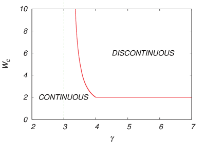
FIG. 5: The value of the minimum cooperativity $W_{c}$ needed for a discontinuous transition, as a function of $\gamma$.

The detailed calculations, reported in Appendix B, give the following results, which provide a complete picture of the model behavior:

• For $\gamma>4$ the transition is continuous if the cooperativity $W=\beta/\alpha$ is sufficiently small, i.e., $W<W_{c}=2$ and the associated exponent is $1/\psi=1$. When $W>W_{c}$ instead the transition is discontinuous. This is in agreement with what is found in Fig. 4. In the marginal case $W=W_{c}$, the transition is still continuous but with critical exponent $1/(\gamma-3)$ for $4<\gamma<5$ and $1/2$ for $\gamma>5$. This last result is consistent with the mean-field treatment in Ref. Chen et al. (2013).

• For $3<\gamma<4$ the limit value $W_{c}$ for the transition to be continuous is always larger than $2$ and assumes a nontrivial dependence on $\gamma$ (see Fig. 5) that continuously interpolates between $2$ for $\gamma\to 4$ and infinity for $\gamma\to 3$. Also the critical exponent changes continuously $1/\psi=1/(\gamma-3)$. Also in this range of $\gamma$ values things are different for marginal cooperativity $W=W_{c}$: in this case $1/\psi=1$ regardless of the value of $\gamma$.

• For $2<\gamma<3$ the threshold vanishes, the transition is continuous for any value of the cooperativity $W$ and the growth of the order parameter for small $\alpha$ is $\alpha^{1/\psi}$, where $1/\psi=(\gamma-2)/(3-\gamma)$.

V Conclusions

In this paper we have performed an analysis of the implications of cooperativity for SIR-like epidemic spreading on power-law degree-distributed networks. First, we have tested the interpretation put forward in Ref. Cai et al. (2015) about the physical origin of the discontinuous epidemic transition occurring in this kind of systems for large cooperativity. Via numerical simulations, we have shown that strong finite system size effects may hide the discontinuity, but that if the system size is large enough the true, hybrid, nature of the transition becomes evident. This provides a strong validation of the physical picture proposed by Cai et al. Cai et al. (2015).

In the second part of the paper we have applied the heterogeneous mean-field theoretical approach to the co–infection dynamics on uncorrelated networks. In this way we have derived an expression for the epidemic threshold, which does not depend on cooperativity, in agreement with simulations. Moreover, the approach allows us to derive, for power-law degree-distributed topologies, the range of cooperativity values for which the transition is continuous and the associated critical exponent. We find a nice confirmation that the discontinuous transition occurs when cooperativity is sufficiently high and local clustering is instead small. An interesting point in this respect regards what happens for scale-free networks, i.e. for $2<\gamma<3$. In such a case HMF theory predicts that the transition is continuous for any value of the cooperativity $W$. This is in agreement with the simulation results for BA networks presented in Ref. Cai et al. (2015); Grassberger et al. (2016) for networks of moderate size. However, one cannot in principle exclude that also for $\gamma<3$ the continuous transition observed in simulations is just a finite size effect. While HMF theory seems to indicate the contrary, the global clustering coefficient Eq. (1) vanishes as the system size diverges also for $\gamma<3$, so that asymptotically there are no short loops in the system. Numerical simulations cannot be conclusive about this question. The issue could be clarified only by a careful analysis of the balance between the relative abundance of short loops (encoded by $C$) and long loops in the network. It remains as a challenging goal.

It is also worth noticing that our theoretical approach is fully general with respect to the value of the infection rates ratio $W=\beta/\alpha$. Therefore our results provide predictions also for competing pathogens, for which $W<1$. In that case our theory predicts always a continuous transition, for any $\gamma$ perfectly analogue to the case of weak cooperativity $1<W<2$.

Mutual cooperation is a very important ingredient also for non-biological spreading processes, such as the diffusion of ideas or the adoption of innovations. The investigation of cooperative effects in general complex contagion dynamics remains a very interesting avenue for future research activity.

Appendix A

In this Appendix, we summarize the connection between bond percolation and the various implementations of the SIR dynamics to allow a proper comparison between theoretical and numerical results. We refer to single-infection SIR in this Appendix.

Bond percolation

In bond percolation on networks, each edge is occupied with probability $T$. The generating function formalism Callaway et al. (2000) provides a solution for bond percolation that is exact for random uncorrelated networks with any degree distribution $P(k)$ in the limit of infinite size $N\to\infty$ Dorogovtsev et al. (2008)

$$T_{c}=\frac{\left\langle{k}\right\rangle}{\left\langle{k^{2}}\right\rangle-\left\langle{k}\right\rangle}.$$ (16)

Notice that for Erdös-Rényi graphs $\left\langle{k^{2}}\right\rangle=\left\langle{k}\right\rangle^{2}+\left\langle{k}\right\rangle$, hence $T_{c}=1/\left\langle{k}\right\rangle$. For Random Regular Graphs of degree $k$: $T_{c}=1/(k-1)$.

SIR in discrete time

Consider the following implementation of the SIR model: at time step $t$ one goes through all nodes in state I. Each neighbor in state S of each I node is infected with probability $p$. When all infected nodes at time step $t$ have been considered, they all go to state R and $t\to t+1$. This model is also called Independent Cascade Model.

The lifetime $\tau$ of each node in the infected state I is fixed deterministically $\tau=1$. With this condition it is possible to exactly map the static properties of the model to bond percolation Newman (2002). One defines as transmissibility the probability for an infected node to pass the infection along one edge before recovering. In the present model this transmissibility is trivially $T=p$. The epidemic process is perfectly equivalent to a bond percolation process starting from a node and iteratively occupying neighbors with transmissibility $T=p$. Therefore the epidemic threshold is

$$p_{c}=T_{c}=\frac{\left\langle{k}\right\rangle}{\left\langle{k^{2}}\right\rangle-\left\langle{k}\right\rangle}.$$ (17)

SIR in continuous time

It is possible to define SIR dynamics also in continuous time. Each infected node has a rate (probability per time unit) $\mu$ to recover. Each edge connecting a node I to a node S has a rate $\alpha$ of transmitting the infection. In this model the lifetime $\tau$ of the infected state is a stochastic variable, distributed as $P(\tau)=\mu\exp(-\mu\tau)$, so that $\left\langle{\tau}\right\rangle=1/\mu$. For this reason, it is not possible to map exactly the model onto bond percolation. However, it is possible to perform an approximate mapping Newman (2002), which turns out to be exact in the determination of the epidemic threshold Pastor-Satorras et al. (2015).

The idea is to compute the average transmissibility $\left\langle{T}\right\rangle$, i.e. the average probability to transmit the infection before recovering. For a given $\tau$ the probability of not transmitting the infection during time $\tau$ is $1-T=\exp(-\alpha\tau)$. Therefore the average transmissibility is

$$\left\langle{T}\right\rangle=1-\int_{0}^{\infty}d\tau P(\tau)\exp(-\alpha\tau).$$ (18)

Inserting the expression for $P(\tau)$ one gets

$$\left\langle{T}\right\rangle=\frac{1}{\mu/\alpha+1}.$$ (19)

The transition will occur when $\left\langle{T}\right\rangle$ equals the expression in Eq. (17), yielding

$$\left(\frac{\alpha}{\mu}\right)_{c}=\frac{\left\langle{k}\right\rangle}{\left\langle{k^{2}}\right\rangle-2\left\langle{k}\right\rangle}.$$ (20)

Notice that this expression is different from the expression for discrete time SIR. Both are exact (in the limit of infinite size) but for different types of dynamics.

In the case of Erdős-Rényi graphs the previous formula implies $(\alpha/\mu)_{c}=\frac{1}{\left\langle{k}\right\rangle-1}$. For Random Regular Graphs instead $(\alpha/\mu)_{c}=\frac{1}{k-2}$.

A consequence of this treatment is that one can pass from the parameter $p$ of the discrete dynamics to the parameter $\alpha/\mu$ of the continuous dynamics (the only relevant parameter) by the relations

$$p=\frac{1}{\mu/\alpha+1}~{}~{}~{}~{}~{}~{}~{}~{}~{}\frac{\alpha}{\mu}=\frac{p}{1-p}.$$ (21)

HMF theory for SIR

The SIR model in the continuous time formulation can be attacked by means of the Heterogeneous Mean-Field (HMF) theory. The HMF theory allows to derive an approximate formula for the epidemic threshold Pastor-Satorras et al. (2015)

$$\left(\frac{\alpha}{\mu}\right)_{c}^{HMF}=\frac{\left\langle{k}\right\rangle}{\left\langle{k^{2}}\right\rangle-\left\langle{k}\right\rangle}.$$ (22)

It is very important to stress that:

• The HMF prediction is not exact. The exact result for continuous dynamics is Eq. (20). This discrepancy is not surprising, as transition points are not universal, they depend on details of the dynamics and are rarely predicted with accuracy by approximate mean-field approaches.

• The HMF prediction for the parameter $\alpha$ in continuous SIR dynamics coincides with the exact threshold for the parameter $p$ of discrete SIR dynamics (Eq. 17). This seems to be just a coincidence.

Appendix B

In this Appendix, we consider the expansion of Eq. (IV) for small $\phi_{\infty}$ and, based on it, we deduce the properties of the transition: its position $\alpha_{c}$, its nature and the associated critical exponent $1/\psi$.

To simplify notation, we write $\phi$ for the stationary value $\phi_{\infty}$ and $m$ for the minimum degree $k_{min}$. Introducing the cooperativity $W=\beta/\alpha$, Eq. (IV) can be rewritten as

$$\phi=\frac{\langle k-1\rangle}{\langle k\rangle}+\frac{1}{\left\langle{k}\right\rangle}\sum_{k}(k-1)P(k)\frac{e^{-W\alpha k\phi}-(W-1)e^{-2\alpha k\phi}}{W-2}$$ (23)

By assuming the explicit form of the degree distribution $P(k)=(\gamma-1)m^{\gamma-1}k^{-\gamma}$ and transforming the sum in a continuous integral, it is possible to rewrite Eq. 23

$$\begin{array}[]{lll}\phi=\frac{\langle k-1\rangle}{\langle k\rangle}\!\!\!&-\frac{\gamma-1}{\langle k\rangle}\frac{W-1}{W-2}\left[\right.&\!\!m(2\alpha m\phi)^{\gamma-2}\Gamma(2-\gamma,2\alpha m\phi)\\ &&\left.\!-(2\alpha m\phi)^{\gamma-1}\Gamma(1-\gamma,2\alpha m\phi)\right]\\ &+\frac{\gamma-1}{\langle k\rangle}\frac{1}{W-2}\left[\right.&\!\!m(W\alpha m\phi)^{\gamma-2}\Gamma(2-\gamma,W\alpha m\phi)\\ &&\left.\!-(W\alpha m\phi)^{\gamma-1}\Gamma(1-\gamma,W\alpha m\phi)\right]\end{array}$$ (24)

where $\Gamma(s,x)=\int_{x}^{\infty}t^{s-1}e^{-t}dt$ is the incomplete Gamma function, that can be expanded as

$$\Gamma(s,x)=\Gamma(s)-x^{s}\sum_{n=0}^{\infty}\frac{(-x)^{n}}{n!(s+n)}\,.$$ (25)

Replacing the expansion in Eq. (24) gives

$$\begin{array}[]{ll}\phi=\frac{\langle k-1\rangle}{\langle k\rangle}\!\!&-\frac{(\gamma-1)}{\langle k\rangle}\frac{W-1}{W-2}\left[m\left((2m\alpha\phi)^{\gamma-2}\Gamma(2-\gamma)-\sum_{n=0}^{\infty}\frac{(-2\alpha m\phi)^{n}}{(2-\gamma+n)n!}\right)-\left((2m\alpha\phi)^{\gamma-1}\Gamma(1-\gamma)-\sum_{n=0}^{\infty}\frac{(-2\alpha m\phi)^{n}}{(1-\gamma+n)n!}\right)\right]+\\ &+\frac{(\gamma-1)}{\langle k\rangle}\frac{1}{W-2}\left[m\left((mW\alpha\phi)^{\gamma-2}\Gamma(2-\gamma)-\sum_{n=0}^{\infty}\frac{(-W\alpha m\phi)^{n}}{(2-\gamma+n)n!}\right)-\left((mW\alpha\phi)^{\gamma-1}\Gamma(1-\gamma)-\sum_{n=0}^{\infty}\frac{(-W\alpha m\phi)^{n}}{(1-\gamma+n)n!}\right)\right]\end{array}$$ (26)

Collecting terms of the same order in $\phi$, and using the identity $\left\langle{k}\right\rangle=m(\gamma-1)/(\gamma-2)$ we get

$$\begin{array}[]{ll}\phi=\!\!&\Gamma(3-\gamma)(2m\alpha)^{\gamma-2}G(W,\gamma-2)\phi^{\gamma-2}+\\ &\!\!\!-\Gamma(2-\gamma)\frac{(2m\alpha)^{\gamma-1}}{m(\gamma-1)/(\gamma-2)}G(W,\gamma-1)\phi^{\gamma-1}+\\ &\!\!\!-\frac{\gamma-2}{m}\sum_{n=1}^{\infty}\frac{(-2m\alpha)^{n}}{n!}\left(\frac{m}{\gamma-(n+2)}-\frac{1}{\gamma-(n+1)}\right)G(W,n)\phi^{n},\end{array}$$ (27)

where we have defined

$$G(W,n)=1-\frac{1}{2}\frac{(W/2)^{n}-1}{W/2-1}\,.$$ (28)

Notice that all terms of zero-th order cancel out.

For $\gamma>4$ the lowest-order terms of the expansion are

$$\begin{array}[]{ll}\phi=&\alpha\left(m\frac{\gamma-2}{\gamma-3}-1\right)\phi+\\ &+\frac{\gamma-2}{\gamma-3}m\alpha^{2}(W-2)\left(m\frac{\gamma-3}{\gamma-4}-1\right)\phi^{2}+O(\phi^{2})\end{array}$$ (29)

The transition point $\alpha_{c}$ is the value for which the linear part vanishes. Therefore

$$\alpha_{c}=\left(m\frac{\gamma-2}{\gamma-3}-1\right)^{-1}\,\,\,\mbox{for}\,\,\,\,\gamma>4\,.$$ (30)

Notice that this expression is nothing else than Eq. (14), $\alpha_{c}=\left\langle{k}\right\rangle/(\left\langle{k^{2}}\right\rangle-\left\langle{k}\right\rangle)$.

In order for the transition to be continuous, Eq. (29) must admit a solution with arbitrary small $\phi$ for $\alpha$ slightly above the transition point $(\alpha-\alpha_{c})/\alpha_{c}=a\phi^{\psi}$, with $a>0$. Inserting this expression into the r.h.s. of Eq. (29) we obtain

$$\phi=\phi(1+a\phi^{\psi})+\frac{\gamma-2}{\gamma-3}m(\alpha\phi)^{2}(W-2)\left(m\frac{\gamma-3}{\gamma-4}-1\right)+O(\phi^{2})$$ (31)

that can be satisfied for $\psi=1$ as long as

$$\frac{\gamma-2}{\gamma-3}m\alpha^{2}_{c}(W-2)\left(m\frac{\gamma-3}{\gamma-4}-1\right)<0.$$ (32)

This occurs for $W<W_{c}=2$, which means $\beta<2\alpha$. Therefore the transition becomes discontinuous for high enough cooperativity, and precisely when the infectivity for the second pathogen is at least twice the one for the single disease.

When the cooperativity $W$ exactly equals its critical value, the coefficient of the term of order $\phi^{2}$ vanishes. The transition can still be continuous but the term $\phi^{1+\psi}$ has to match the next order term in the expansion. For $4<\gamma<5$ such a term is $\phi^{\gamma-2}$ so that $\psi=\gamma-3$; for $\gamma>5$ the next order term is $\phi^{3}$, implying $\psi=2$. In this last case the order parameter grows as $(\alpha-\alpha_{c})^{1/2}$ in agreement with the mean-field results obtained in Ref. Chen et al. (2013).

For $3<\gamma<4$, the transition point is still given by Eq. (30). Assuming again $(\alpha-\alpha_{c})/\alpha_{c}=a\phi^{\psi}$ the lowest orders of Eq. (27) are

$$\phi=\phi(1+a\phi^{\psi})+\Gamma(3-\gamma)(2m\alpha\phi)^{\gamma-2}G(W,\gamma-2)+O(\phi^{2})$$ (33)

Eq. (33) can be satisfied if the term $a\phi^{1+\psi}$ matches the term of order $\phi^{\gamma-2}$. This is possible if $\psi=\gamma-3$ and if the coefficient $\Gamma(3-\gamma)(2m\alpha)^{\gamma-2}G(W,\gamma-2)$ is negative. Since for this range of $\gamma$, $\Gamma(3-\gamma)$ is negative, the condition for the transition to be continuous is $G(W,\gamma-2)>0$. Therefore, for a given $3<\gamma<4$ the transition is continuous only for $W\leq W_{c}$, with $W_{c}$ determined by

$$G(W_{c},\gamma-2)=0\,,$$ (34)

otherwise the transition is discontinuous. Figure 5 displays how $W_{c}$ depends on $\gamma$. Starting from $\gamma=4$ and reducing $\gamma$ the value of the cooperativity $W_{c}$ needed for the transition to become discontinuous grows and it diverges as $\gamma\rightarrow 3$. The critical exponent for the continuous transition is $1/\psi=1/(\gamma-3)$ for $W<W_{c}$. For $W$ exactly equal to $W_{c}$ the coefficient of the term of order $\phi^{\gamma-3}$ vanishes, therefore the continuous transition is possible only when the term of order $\phi^{1+\psi}$ is matched by the next term in the expansion, which for $3<\gamma<4$ is given by the term in $\phi^{2}$, yielding $\psi=1$.

Finally, let us consider the case $2<\gamma<3$. In this range the threshold is $\alpha_{c}=0$ and we assume $\alpha=a^{\prime}\phi^{\psi}$. The lowest order of the r.h.s. of Eq. (27) is $\Gamma(3-\gamma)(2ma^{\prime}\phi^{\psi})^{\gamma-2}G(W,\gamma-2)\phi^{\gamma-2}$. Since now $\Gamma(3-\gamma)>0$ and $G(W,\gamma-2)>0$ for any $W$ there is always a solution (i.e., the transition is always continuous) provided $(1+\psi)(\gamma-2)=1$, implying that the critical exponent is $1/\psi=(\gamma-2)/(3-\gamma)$.

References

- Pastor-Satorras et al. (2015) R. Pastor-Satorras, C. Castellano, P. Van Mieghem, and A. Vespignani, Rev. Mod. Phys. 87, 925 (2015).
- Newman (2005a) M. E. J. Newman, Phys. Rev. Lett. 95, 108701 (2005a).
- Funk and Jansen (2010) S. Funk and V. A. A. Jansen, Phys. Rev. E 81, 036118 (2010).
- Marceau et al. (2011) V. Marceau, P.-A. Noël, L. Hébert-Dufresne, A. Allard, and L. J. Dubé, Phys. Rev. E 84, 026105 (2011).
- Miller (2013) J. C. Miller, Phys. Rev. E 87, 060801 (2013).
- Taubenberger and Morens (2006) J. K. Taubenberger and D. M. Morens, Emerging Infectious Diseases 12, 15 (2006).
- Morens et al. (2008) D. M. Morens, J. K. Taubenberger, and A. S. Fauci, The Journal of Infectious Diseases 198, 962 (2008).
- Brundage and Shanks (2008) J. F. Brundage and G. Shanks, Emerg. Infect Dis. 14, 1193 (2008).
- Sulkowski (2008) M. S. Sulkowski, Journal of Hepatology 48, 353 (2008).
- Newman and Ferrario (2013) M. E. J. Newman and C. R. Ferrario, PLoS ONE 8, e71321 (2013).
- Kermack and McKendrick (1927) W. O. Kermack and A. G. McKendrick, Proc. R. Soc. Lond. A 115, 700 (1927).
- Chen et al. (2013) L. Chen, F. Ghanbarnejad, W. Cai, and P. Grassberger, EPL (Europhysics Letters) 104, 50001 (2013).
- Janssen and Stenull (2016) H.-K. Janssen and O. Stenull, EPL (Europhysics Letters) 113, 26005 (2016).
- Cai et al. (2015) W. Cai, L. Chen, F. Ghanbarnejad, and P. Grassberger, Nature physics 11, 936 (2015).
- Grassberger et al. (2016) P. Grassberger, L. Chen, F. Ghanbarnejad, and W. Cai, Phys. Rev. E 93, 042316 (2016).
- Goltsev et al. (2006) A. V. Goltsev, S. N. Dorogovtsev, and J. F. F. Mendes, Phys. Rev. E 73, 056101 (2006).
- Parisi and Rizzo (2008) G. Parisi and T. Rizzo, Phys. Rev. E 78, 022101 (2008).
- Sanz et al. (2014) J. Sanz, C.-Y. Xia, S. Meloni, and Y. Moreno, Phys. Rev. X 4, 041005 (2014).
- Azimi-Tafreshi (2016) N. Azimi-Tafreshi, Phys. Rev. E 93, 042303 (2016).
- Chen et al. (2016) L. Chen, F. Ghanbarnejad, and D. Brockmann, ArXiv e-prints (2016), arXiv:1603.09082 [physics.soc-ph] .
- Catanzaro et al. (2005) M. Catanzaro, M. Boguñá, and R. Pastor-Satorras, Phys. Rev. E 71, 027103 (2005).
- Newman (2005b) M. E. J. Newman, “Random graphs as models of networks,” in Handbook of Graphs and Networks (Wiley-VCH Verlag GmbH & Co. KGaA, 2005) pp. 35–68.
- Pastor-Satorras and Vespignani (2001) R. Pastor-Satorras and A. Vespignani, Phys. Rev. Lett. 86, 3200 (2001).
- Moreno et al. (2002) Y. Moreno, R. Pastor-Satorras, and A. Vespignani, The European Physical Journal B - Condensed Matter and Complex Systems 26, 521 (2002).
- Boguñá et al. (2003) M. Boguñá, R. Pastor-Satorras, and A. Vespignani, in Statistical Mechanics of Complex Networks, Lecture Notes in Physics, Vol. 625, edited by R. Pastor-Satorras, J. M. Rubí, and A. D.-G. a (Springer Verlag, Berlin, 2003) pp. 127–147.
- Callaway et al. (2000) D. S. Callaway, M. E. J. Newman, S. H. Strogatz, and D. J. Watts, Phys. Rev. Lett. 85, 5468 (2000).
- Dorogovtsev et al. (2008) S. N. Dorogovtsev, A. V. Goltsev, and J. F. F. Mendes, Rev. Mod. Phys. 80, 1275 (2008).
- Newman (2002) M. E. J. Newman, Phys. Rev. E 66, 016128 (2002).