Simple fully non-local density functionals for the electronic repulsion energy

Abstract

From a simplified version of the mathematical structure of the strong coupling limit of the exact exchange-correlation functional, we construct an approximation for the electronic repulsion energy at physical coupling strength, which is fully non-local. This functional is self-interaction free and yields energy densities within the definition of the electrostatic potential of the exchange-correlation hole that are locally accurate and have the correct asymptotic behavior. The model is able to capture strong correlation effects that arise from chemical bond dissociation, without relying on error cancellation. These features, which are usually missed by standard DFT functionals, are captured by the highly nonlocal structure, which goes beyond the Jacob’s ladder framework for functional construction, by using integrals of the density as the key ingredient. Possible routes for obtaining the full exchange-correlation functional by recovering the missing kinetic component of the correlation energy are also implemented and discussed.

The widespread success of Kohn–Sham density-functional theory (KS DFT)Kohn and Sham (1965); Cohen, Mori-Sánchez, and Yang (2012); Burke (2012); Becke (2014) across various chemical and physical disciplines has been also accompanied by spectacular failures,Cohen, Mori-Sánchez, and Yang (2012) reflecting fundamental issues in the present density functional approximations (DFAs) for the exchange–correlation (XC) functional. Well-known examples are the paradigmatic case of the dissociation curves of the H₂ and H${}_{2}^{+}$ molecules.Savin (1996); Cohen, Mori-Sánchez, and Yang (2012) The usual DFAs approach to construct XC functionals consists in making an ansatz in terms of “Jacob’s ladder” ingredients: Perdew et al. (2005); Becke (2014); Medvedev et al. (2017); Hammes-Schiffer (2017) the local density, its gradient, its laplacian and/or KS kinetic energy density, up to occupied and virtual KS orbitals. While this strategy has been very successful for moderately correlated systems (see, e.g., Refs. Burke, 2012; Becke, 2014; Zhao and Truhlar, 2008; Sun et al., 2016; Erhard, Bleiziffer, and Görling, 2016), it has failed so far when correlation effects become important (e.g., in stretched bonds, but also at equilibrium gemoetries when partially filled $d$ and $f$ subshells are present). This fact suggests that a different approach to DFAs is needed to address the problem of strong correlation.Burke (2012); Cohen, Mori-Sánchez, and Yang (2012); Mori-Sánchez and Cohen (2014); Cohen, Mori-Sanchez, and Yang (2008); Vuckovic et al. (2016)

The strong-interaction limit of DFTSeidl (1999); Seidl, Gori-Giorgi, and Savin (2007); Gori-Giorgi, Vignale, and Seidl (2009); Buttazzo, De Pascale, and Gori-Giorgi (2012) provides information on how the exact XC functional depends on the density in a well defined mathematical limit, which is relevant for strong correlation. The thorough explorations of this limit reveal a mathematical structure totally different from that of Jacob’s ladder ingredients. Instead of the local density, density derivatives or KS orbitals, in this limit we see that certain integrals of the density play a crucial role, encoding highly nonlocal information, Seidl (1999); Seidl, Gori-Giorgi, and Savin (2007); Gori-Giorgi, Vignale, and Seidl (2009) embodied in the so-called strictly-correlated electrons (SCE) functional.Seidl (1999); Seidl, Gori-Giorgi, and Savin (2007); Gori-Giorgi, Vignale, and Seidl (2009) This functional appears to be well–equipped for solving long-standing DFAs problems: it is self–interaction free, it captures the physics of charge localization due to strong correlation without resorting to symmetry breaking,Malet et al. (2013); Mendl, Malet, and Gori-Giorgi (2014); Malet et al. (2015) and its functional derivative displays (in the low-density asymptotic limit) a discontinuity on the onset of fractional particle number.Mirtschink, Seidl, and Gori-Giorgi (2013) Despite these appealing features, there are two main obstacles to the routine use of the SCE functional: its availability is restricted to small systemsSeidl, Gori-Giorgi, and Savin (2007); Vuckovic et al. (2015) and its energies are way too low for most of physical and chemical systems.Malet et al. (2013, 2014); Chen, Friesecke, and Mendl (2014); Vuckovic et al. (2015) The nonlocal radius (NLR) functional,Wagner and Gori-Giorgi (2014) and the newer shell–modelBahmann, Zhou, and Ernzerhof (2016) are inspired to the SCE functional form and retain only some of its non-locality. They are readily available,Bahmann, Zhou, and Ernzerhof (2016) but, being approximations to the SCE functional, their energies are also too low with respect to those of chemical systems.Wagner and Gori-Giorgi (2014); Bahmann, Zhou, and Ernzerhof (2016) The information encoded in the SCE functional or its approximations can be combined with the complementary information from the weak coupling limit. This has been recently used for constructing XC functionals from a local interpolation along the adiabatic connection.Vuckovic et al. (2016); Zhou, Bahmann, and Ernzerhof (2015); Bahmann, Zhou, and Ernzerhof (2016); Vuckovic et al. (2017) Although this approach is promising for treating strong correlation within the realm of DFT,Vuckovic et al. (2016) it can still easily over-correlate (for example for stretched bonds it overcorrelates the fragments), again because the SCE (exact or approximate) quantities are often far from the physical ones.Vuckovic et al. (2017)

Nonetheless, the way in which the information encoded in the density is transfomed into an electron-electron repulsion energy in the SCE functional is very intriguing, with many physical appealing features.Seidl, Gori-Giorgi, and Savin (2007); Malet and Gori-Giorgi (2012); Lani et al. (2016); Seidl et al. (2017) Motivated by this observation, in this letter we use the SCE mathematical structure to devise a new way to design fully non-local approximate density functionals for the electronic interaction energy at the physical coupling strength. Capturing the main structural motives of the SCE functional, we preserve many of its appealing features, but with repulsion energies that are much closer to those of physical systems. Moreover, besides accurate total repulsion energies, our model provides energy densities within the definition of the electrostratic potential of the XC hole that are also locally very close to exact ones, making it an ideal tool for the developement of functionals that use the exact exchange energy density, like hyperGGA’sPerdew and Schmidt (2001); Becke (2005); Perdew et al. (2008); Kong and Proynov (2015) or local hybrids.Jaramillo, Scuseria, and Ernzerhof (2003); Arbuznikov and Kaupp (2007) In other words, it is knownClementi and Chakravorty (1990); Becke (1993); Perdew and Schmidt (2001); Perdew et al. (2008) that in order to use the exact exchange energy density we need a fully non-local correlation functional compatible with it. It is the purpose of this work to provide a new strategy to build this fully non-local functional at a computational cost similar to the one of the exact exchange energy density.

In order to explain our construction we have to first quickly review some basic DFT equations. An exact expression for the XC energy can be obtained from the density-fixed adiabatic connection formalism (AC):Langreth and Perdew (1975); Gunnarsson and Lundqvist (1976)

$$E_{xc}[\rho]=\int_{0}^{1}W_{\lambda}[\rho]\mathrm{d}\lambda,$$ (1)

where $W_{\lambda}[\rho]$ is the global (i.e., integrated over all space) AC integrand:

$$W_{\lambda}[\rho]=\langle\Psi_{\lambda}[\rho]|\hat{V}_{ee}|\Psi_{\lambda}[\rho]\rangle-U[\rho].$$ (2)

The wavefunction $\Psi_{\lambda}[\rho]$ depends on the positive coupling constant $\lambda$ and minimizes $\langle\hat{T}+\lambda\hat{V}_{ee}\rangle$, while integrating to $\rho({\bf r})$, the density of the physical system ($\lambda=1$). This way, AC links the KS non–interacting state described by $\Psi_{0}[\rho]$ and the physical state described by $\Psi_{1}[\rho]$. It also further connects the physical and the SCE state, i.e. the state of perfect electron correlation, corresponding to the limit $\lambda\to\infty$. The XC energy densities along the adiabatic connection (i.e., position-dependent quantities $w_{\lambda}({\bf r})$ that integrate to $W_{\lambda}[\rho]$ when multiplied by the density) are not uniquely defined and therefore we have to be specific on their gauge.Burke, Cruz, and Lam (1998); Cruz, Lam, and Burke (1998); Tao et al. (2008); Vuckovic et al. (2016, 2017) A physically sound gauge often considered in DFT is the one of the electrostatic potential of the XC hole.Becke (2005); Becke and Johnson (2007); Perdew et al. (2008); Vuckovic et al. (2016) Within this gauge we can express the $\lambda$-dependent energy density in terms of the corresponding spherically-averaged XC holeBecke (2005); Perdew et al. (2008); Gori-Giorgi, Angyan, and Savin (2009); Vuckovic et al. (2016) $h_{\rm xc}^{\lambda}({\bf r},u)$ obtained from $|\Psi_{\lambda}[\rho]|^{2}$,

$$w_{\lambda}({\bf r})=\frac{1}{2}\int_{0}^{\infty}\frac{h_{\rm xc}^{\lambda}({\bf r},u)}{u}4\pi u^{2}\mathrm{d}u,$$ (3)

where $u=\left|{\bf r}-{\bf r}^{\prime}\right|$ is the distance from a reference electron in ${\bf r}$. In the SCE ($\lambda\to\infty$) limit the energy density $w_{\lambda}({\bf r})$ in the gauge of Eq. (3) has the exact formMirtschink, Seidl, and Gori-Giorgi (2012)

$$w_{\infty}({\bf r})=\frac{1}{2}\sum_{i=2}^{N}\frac{1}{|{\bf r}-{\bf f}_{i}([\rho];{\bf r})|}-\frac{1}{2}v_{H}({\bf r}),$$ (4)

where $v_{H}({\bf r})$ is the Hartree potential and the co-motion functions ${\bf f}_{i}([\rho];{\bf r})$ are non-local functionals of the density that give the positions of the remaining $N-1$ electrons when one electron is at position ${\bf r}$.Seidl (1999); Seidl, Gori-Giorgi, and Savin (2007); Seidl et al. (2017) From Eq. (4) we see that in the $\lambda\to\infty$ limit the energy density $w_{\infty}({\bf r})$ is fully determined by the distances $R_{i}^{\rm SCE}([\rho];{\bf r})=|{\bf r}-{\bf f}_{i}([\rho];{\bf r})|$ between a reference electron in ${\bf r}$ and the remaining $N-1$ ones. For example, in the case of one-dimensional systems, the distances $R_{i}^{\rm SCE}([\rho];x)$ can be constructed exactlySeidl (1999); Colombo, De Pascale, and Di Marino (2015) from the equations (with $i=2,\dots,N$)

$$\int_{x}^{f_{i}(x)}\rho(x^{\prime})\,{\rm d}x^{\prime}=i-1,\qquad R_{i}^{\rm SCE}(x)=|x-f_{i}(x)|,$$ (5)

which can be solved in terms of the function $N_{\rm 1D}(x)=\int_{-\infty}^{x}\rho(x^{\prime})\,{\rm d}x^{\prime}$ and its inverse $N_{\rm 1D}^{-1}(y)$.Seidl (1999); Malet and Gori-Giorgi (2012); Malet et al. (2013) We see that in this limit each electron is separated by the closest one by a piece of density that integrates exactly to 1 (in other words, fluctuations are totally suppressed in the limit of extreme correlation), with the key ingredient being the amount of expected electrons between two electronic positions.

In this work we propose a way to generalize the SCE form of Eq. (4) by using $\lambda$-dependent distances (or “radii”) $R_{i}^{\lambda}([\rho];{\bf r})$ that will take into account the effect of fluctuations, which are not as suppressed as in the extreme SCE case. Thus, our “multiple-radii functional” (${\rm{MRF}}$) energy density reads as

$$w_{\lambda}^{\rm{MRF}}({\bf r})=\frac{1}{2}\sum_{i=2}^{N}\frac{1}{R_{i}^{\lambda}([\rho];{\bf r})}-\frac{1}{2}v_{H}({\bf r}).$$ (6)

As we shall see, we will determine the $R_{i}^{\lambda}([\rho];{\bf r})$ by using a simplified version of the same kind of integrals of the density that appear in the SCE limit, introducing the average effect of fluctuations by reducing the amount of expected charge between two electronic positions. Before coming to the details of the $R_{i}^{\lambda}([\rho];{\bf r})$ construction, we remark that Eq. (6) can be also derived from the following model for the spherically-averaged pair-density

$$P_{2,\lambda}^{{\rm{MRF}}}([\rho];{\bf r},u)=\frac{1}{4\pi u^{2}}\sum_{i=2}^{N}\rho({\bf r})\delta\big{(}u-R_{i}^{\lambda}({\bf r})\big{)},$$ (7)

where $\delta$ is the Dirac delta function. Given that the model of Eq. (7) is properly normalised, the corresponding $\lambda$-dependent XC hole satisfies the sum rule, integrating to $-1$ electron.

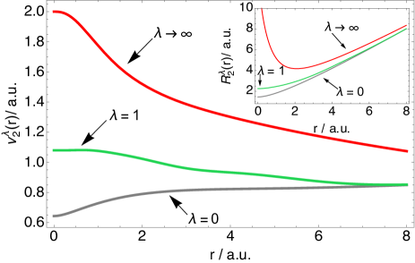
Figure 1: The $\nu_{2}^{\lambda}({\bf r})$ quantity of Eq (10) and the corresponding $R_{2}^{\lambda}({\bf r})$ radius at different coupling strengths for the hydride ion obtained from Eq. (11) using accurate xc energy densities $w_{\lambda}({\bf r})$ from Refs. Irons and Teale, 2015; Vuckovic et al., 2016.

We now turn to the construction the radii $R_{i}^{\lambda}([\rho];{\bf r})$. Motivated by the structure of Eq. (5), and similarly to the recent non-local approximations for the SCE functional for three-dimensional systems,Wagner and Gori-Giorgi (2014); Bahmann, Zhou, and Ernzerhof (2016) we introduce the spherically averaged density $\tilde{\rho}({\bf r},u)$ around a position ${\bf r}$,

$$\tilde{\rho}({\bf r},u)=\int\frac{1}{4\pi}\rho({\bf r}+\mathbf{u})\mathrm{d}\Omega_{\mathbf{u}},$$ (8)

and the function $N_{e}({\bf r},u)$,

$$N_{e}({\bf r},u)=\int_{0}^{u}4\pi x^{2}\,\tilde{\rho}({\bf r},x)\,{\rm d}x.$$ (9)

These functions have been studied and efficiently implemented by Ernzerhof and co-workers.Antaya, Zhou, and Ernzerhof (2014); Zhou, Bahmann, and Ernzerhof (2015); Bahmann, Zhou, and Ernzerhof (2016) We now want to find a physical approximation for the crucial quantities

$$\nu_{i}^{\lambda}({\bf r})=N_{e}({\bf r},R_{i}^{\lambda}({\bf r})),\qquad i=2,\dots,N$$ (10)

which give the expected number of electrons in a sphere of radius $R_{i}^{\lambda}({\bf r})$ centered at the reference electron in ${\bf r}$. We notice at this point that in an inhomogeneous system, even one-dimensional, it is not possible to write the exact SCE radii explicitly in terms of the function $N_{e}({\bf r},u)$ obtained by spherically averaging the density around a reference electron in ${\bf r}$ as in Eq. (8). An exception is an homogeneous 1D system, in which $\nu_{2}^{\rm SCE}=\nu_{3}^{\rm SCE}=2$, $\nu_{4}^{\rm SCE}=\nu_{5}^{\rm SCE}=4$, etc.

At the physical interaction strength $\lambda=1$, we expect a situation in which this extreme correlation is reduced, with all the $\nu_{i}$ close to $i-1$. To illustrate this fact, we consider first an $N=2$ system, for which we have only one radius, $R_{2}^{\lambda}$, which from Eq. (6) will be equal to

$$R_{2}^{\lambda}({\bf r})=\frac{1}{v_{H}({\bf r})+2w_{\lambda}({\bf r})},$$ (11)

showing that, for $N=2$, $R_{2}^{\lambda}({\bf r})$ is the screening length associated with the Hartree-exchange-correlation potential when its response part is removed.van Leeuwen, Gritsenko, and Baerends (1995); Gritsenko and Baerends (1996); Gritsenko, Mentel, and Baerends (2016) Given that for two-electron systems highly accurate $w_{\lambda}({\bf r})$ have been computed,Irons and Teale (2015); Vuckovic et al. (2016) we can use Eq. (11) to obtain the ‘exact’ $R_{2}^{\lambda}({\bf r})$. In Fig. 1 we show the corresponding $\nu_{2}^{\lambda}({\bf r})$ for the hydride ion at $\lambda=0$, $\lambda=1$, $\lambda\to\infty$. We clearly see that in the physical system $\nu_{2}^{\lambda=1}({\bf r})$ is much closer to 1 than in the SCE extreme case, which allows for much larger numbers $\nu_{2}^{\infty}({\bf r})$, getting equal to 2 at the nucleus, as in the homogeneous 1D solution.

It is clear that there are several ways to define approximations for $\nu_{i}^{\lambda}({\bf r})$, using different ingredients. Here, our aim is to show that already very simple approximations can yield rather accurate results, and we focus on the physical $\lambda=1$ case. As said, we expect that $\nu_{2}^{\lambda=1}({\bf r})\approx 1,\;\nu_{3}^{\lambda=1}({\bf r})\approx 2,\dots$, and we write

$$\nu_{i}^{1}({\bf r})=i-1+\sigma_{i}({\bf r}),\qquad i=2,\dots,N,$$ (12)

yielding for the radii $R_{i}^{\lambda=1}({\bf r})$ the equations

$$R_{i}^{1}({\bf r})=N_{e}^{-1}({\bf r},i-1+\sigma_{i}({\bf r})),\qquad i=2,\dots,N,$$ (13)

with $\sigma_{i}({\bf r})$ being the fluctuation function, which can push away or bring closer the $i$-th electron to the reference one with respect to the expected distance $a_{i}({\bf r})=N_{e}^{-1}({\bf r},i-1)$. In this first model, we consider only the case in which the $i$-th electron is pushed further, because for this case we can use again the mathematical structure of the SCE functional as a guide. More general models will be explored in future works. From the SCE theory for spherically symmetric systems,Seidl, Gori-Giorgi, and Savin (2007); Seidl et al. (2017) we know that the derivative of the radial co-motion function $f_{i}(r)$ at point $r$ is inversely proportional to $4\pi f_{i}(r)^{2}\rho(f_{i}(r))$. We thus introduce the quantity $S_{i}({\bf r})$

$$S_{i}({\bf r})=\frac{\partial N_{e}({\bf r},u)}{\partial u}\Big{|}_{u=N_{e}^{-1}({\bf r},i-1)}=4\pi a_{i}({\bf r})^{2}\,\tilde{\rho}({\bf r},a_{i}({\bf r})),$$ (14)

which, in analogy to the SCE structure, provides information on the derivative of the $R_{i}^{1}({\bf r})$ at $\sigma_{i}=0$. When $S_{i}({\bf r})$ is small, the derivative of the $R_{i}({\bf r})$ will be very large, and we expect the electron to be pushed further, with $\sigma_{i}$ approaching the average value $1/2$ (which is exactly in between two expected positions). When $S_{i}({\bf r})$ is large, the derivative of $R_{i}({\bf r})$ is very small and we expect it to stay close to $\sigma_{i}=0$ (or even become slightly negative, a possibility not considered here). Thus, for constructing the ${\rm{MRF}}$ functional at the full coupling strength, hereinafter the ${\rm{MRF}}$-1 functional, $W_{1}^{\rm{MRF}}[\rho]=\int\rho({\bf r})w_{1}^{\rm{MRF}}({\bf r})d{\bf r}$, we use a simple gaussian ansatz

$$\sigma_{i}({\bf r})=\frac{1}{2}\mathrm{e}^{-b\,S_{i}({\bf r})^{2}},$$ (15)

where $b=5$ has been chosen to optimize the He atom $W_{1}[\rho]$. Equations (6), (8), (9) and (12)-(15) completely define $w_{1}^{\rm{MRF}}({\bf r})$.

Table 1: Atomic (ionic) repulsion energies $W_{1}[\rho]$ obtained by the MRF-1 model and PBE are compared to reference $W_{1}[\rho]$, obtained with Gamess-US package Schmidt et al. (1993) using full-CI (for the first four systems) and CCSD wavefunctions (other systems). The aug-cc-pCVXZ basis set of DunningDunning (1989) has been used ($X=6$ for He and H^-, $X=5$ for F^- and Ne, $X=T$ for Be and Li^- and $X=Q$ for the other atoms). The SCE values $W_{\infty}[\rho]$ computed from the same densities are also reported.

atom/ion	Reference	MRF-1	PBE	SCE
He	-1.1029	-1.1844	-1.1047	-1.4982
H-	-0.4532	-0.4681	-0.4413	-0.5689
Be	-2.8341	-2.8044	-2.8430	-4.0195
Li-	-1.9462	-2.1170	-1.9617	-2.7308
F-	-10.889	-10.741	-10.997	-16.940
Ne	-12.765	-12.823	-12.876	-20.041
Mg	-16.701	-16.365	-16.913	-26.709
Cl-	-28.89	-28.48	-29.19	-47.26
Ar	-31.35	-31.19	-31.68	-51.49
Ca	-35.60	-35.92	-36.85	-60.34
MAE	-	0.17	0.24	-

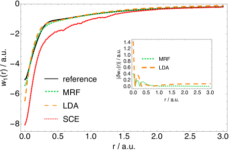
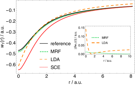
Figure 2: Energy densities at full coupling strength $w_{1}(r)$ as a function of distance from the nucleus, $r$/a.u., obtained from the present model (MRF), from the local-density approximation (LDA),Perdew and Wang (1992) and from the strictly-correlated electrons functional (SCE), all evaluated on accurate densities, for Ne (upper panel) and H^- (lower panel). The reference $w_{1}(r)$ are obtained at the full-CI and CCSD level of theory, as in Refs. Mirtschink, Seidl, and Gori-Giorgi, 2012; Vuckovic et al., 2016, by using the aug-cc-pCVTZ and aug-cc-pV6Z basis setsDunning (1989) for Ne and H^-, respectively. Insets show the absolute error of approximate energy densities, $\delta w_{1}(r)=w_{1}-w_{1}^{\rm apx}(r)$.

In Table 1 we compare $W_{1}[\rho]$ obtained with the MRF-1 model with corresponding reference values (full-CI/CCSD), PBE and SCE ones ($W_{\infty}[\rho]$) for several closed-shell atomic (ionic) systems evaluated on accurate (CCSD) densities. The PBE values have been obtained by using the scaling relationLevy and Perdew (1985, 1993), with $\rho_{\gamma}({\bf r})=\gamma^{3}\rho(\gamma\,{\bf r})$,

$$W_{1}^{\rm DFA}[\rho]=E_{x}^{\rm DFA}[\rho]+2E_{c}^{\rm DFA}[\rho]-\frac{\partial E_{c}^{\rm DFA}[\rho_{\gamma}]}{\partial\gamma}\Big{|}_{\gamma=1}.$$ (16)

From Table 1 we can see that our model, even with the very simple ansatz for $\sigma_{i}({\bf r})$ of Eq. (15), gives repulsion energy much closer to the physical ones with respect to SCE. Their quality is comparable to that of PBE, with MAE somewhat smaller (0.17 a.u. vs. 0.24 a.u.). The purpose here is not to reach high accuracy (which requires optimization and further studies of the $R_{i}$), but to show that functional approximations based on modeling the quantity $\sigma_{i}({\bf r})$ is a very promising strategy, because already a primitive non-optimized model performs very well. Even more interesting than the global $W_{1}^{\rm{MRF}}[\rho]$ values are the energy densities: in Fig. 2 we compare $w_{1}^{\rm MRF}({\bf r})$ with the reference $w_{1}({\bf r})$ for the neon atom (top panel) and the hydride ion (bottom panel). We also show $w_{1}({\bf r})$ obtained with the LDA functional from the PW92 parametrisation,Perdew and Wang (1992); March (1958) $w_{1}^{\rm LDA}(r_{s})=\frac{1}{r_{s}}\frac{\partial}{\partial{r_{s}}}\big{(}{r_{s}}^{2}\epsilon_{xc}(r_{s})\big{)}$. We see that $w_{1}^{\rm MRF}({\bf r})$ is in good agreement with the reference $w_{1}({\bf r})$ in the case of Ne, but also in the more correlated caseMirtschink, Seidl, and Gori-Giorgi (2012); Vuckovic et al. (2016) of H^-, again improving dramatically with respect to SCE. From the insets of the same figure we can see that the local error of our model is very small, vanishing for large ${\bf r}$ due to the correct $-\frac{1}{2|{\bf r}|}$ asymptotic behaviour, arising from the proper normalization of Eq. (7). The availability of DFAs energy densities in this gauge is rather limited, and beyond LDA it is restricted to few approximationsBecke and Roussel (1989); Tao, Bulik, and Scuseria (2016) to the exchange energy density ($\epsilon_{x}({\bf r})=w_{0}({\bf r})$). For instance, the gauge incompatibilityPerdew et al. (2014) of the generalized gradient approximation (GGA) exchange energy densities and the exact $\epsilon_{x}({\bf r})$, which is in the gauge of Eq. (3), has been a major hurdle for the development of local hybrid DFAs.Jaramillo, Scuseria, and Ernzerhof (2003); Arbuznikov and Kaupp (2007)

The main point of introducing the full non-local dependence is of course to treat static and strong correlation. In Fig. 3 we show the energy density $w_{1}^{\rm MRF}({\bf r})$ for the H₂ molecule at different bond lengths $L_{b}$ along the internuclear axis, compared with accurate ones from Ref. Vuckovic et al., 2016. For comparison, we also show $w_{1}({\bf r})$ obtained from the interpolation model of Liu and Burke (LB)Liu and Burke (2009) applied to energy densities, with the exact $w_{0}({\bf r})$, $w^{\prime}_{0}({\bf r})$ and $w_{\infty}({\bf r})$ as input ingredients.Vuckovic et al. (2016) As we can see from Fig. 3, in the equilibrium region the MRF-1 energy densities are still somewhat lower than the reference ones, whereas the LB is highly accurate, as it is also the case with atoms.Vuckovic et al. (2016, 2017) However, we can also see that in the stretched case ($L_{b}=10$ a.u.) the MRF-1 energy densities are very accurate, even more accurate than the LB interpolated ones (note again that they use the exact $w_{0}({\bf r})$, $w^{\prime}_{0}({\bf r})$ and $w_{\infty}({\bf r})$ as input for the interpolation, whose error is already small). While in the stretched H₂ molecule the static correlation effects are dominant, at intermediate bond lengths, around $L_{b}\sim 5.0$ a.u., there is a subtle interplay between dynamic and static correlation effects.Vuckovic et al. (2017) This region can be even more challenging for DFAs than the stretched case, given that certain DFAs which dissociate H₂ correctly fail in this scenario yielding a positive “bump” (see, e.g., Refs Fuchs et al., 2005; Peach et al., 2008; Vuckovic et al., 2016; Zhang et al., 2016). We can see that the MRF-1 energy densities are very accurate at $L_{b}=5.0$ a.u., hardly distinguishable from the reference ones.

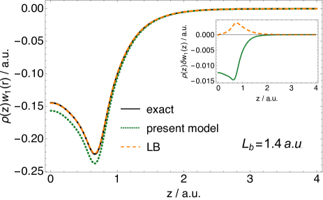
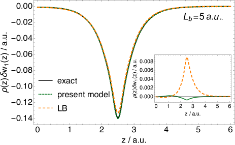
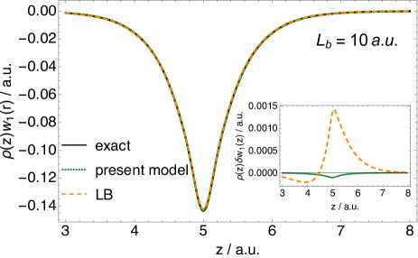
Figure 3: Energy densities at full coupling strength as a function of the distance from the bond midpoint $z$ along the internuclear axis for the H₂ molecule at different bond-lengths $L_{b}$ obtained with MRF-1 using accurate FCI/aug-cc-pCVTZ densities. Reference energy densities and those obtained with the LB local interpolation scheme are from Ref. Vuckovic et al., 2016.

In Fig. 4 we show the dissociation curve for the H₂ molecule obtained using the MRF-1 functional evaluated on the accurate FCI/aug-cc-pCVTZ densities. We can see that around equilibrium MRF-1 underestimates the total energy, because it misses the positive kinetic correlation component $T_{c}[\rho]$ and slightly underestimates the exact $W_{1}[\rho]$, as already shown in Fig. 3. Despite missing $T_{c}[\rho]$, MRF-1 dissociates H₂ correctly, because $T_{c}[\rho]$ vanishes as the H₂ dissociates into atoms. To recover the missing $T_{c}[\rho]$ component, one can combine $W_{1}^{\rm MRF}[\rho]$ with the quantities from the weak coupling limit, namely $W_{0}[\rho]$ and $W^{\prime}_{0}[\rho]$, to interpolate $W_{\lambda}[\rho]$ and thus obtain $E_{\rm xc}[\rho]$. For this purpose, we employ a very simple interpolation form, the two-legged representation,Burke, Ernzerhof, and Perdew (1997); Vuckovic et al. (2016, 2017) which has recently been used to construct a tight lower bound to correlation energies.Vuckovic et al. (2017) This form reads as

$$W_{\lambda}[\rho] =\begin{cases}W_{0}[\rho]+\lambda W^{\prime}_{0}[\rho],&\lambda\leqslant X_{c}\\ W_{1}[\rho],&\lambda>X_{c}\end{cases}$$ (17a)

$$X_{c} =\frac{W_{1}[\rho]-W_{0}[\rho]}{W^{\prime}_{0}[\rho]}.$$ (17b)

As in this work we use $W_{1}^{\rm MRF}[\rho]$ as an approximation to $W_{1}[\rho]$, we call this approach the “2-leg MRF”, and from Fig. 4 we can see that it substantially improves the MRF-1 energies. In this case very similar results are obtained if we do the interpolation on the energy densities rather than on integrated quantities. Besides dissociating correctly H₂, the dissociation of H${}_{2}^{+}$ is also correctly described within the MRF-1 and 2-leg MRF approaches, because our model of Eq. (7) is equal to $0$ for all $N=1$ systems.

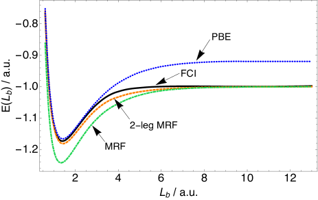
Figure 4: The H₂ molecule dissociation curve as a function of the internuclear distance $L_{b}$/a.u. obtained with the MRF-1 and 2-leg MRF approaches presented in this work, compared to restricted PBE and FCI. All the curves have been obtained using the aug-cc-pCVTZ basis setDunning (1989)

Finally, one may wonder if the MRF would encounter problems for extended systems. As a paradigmatic example, we consider the uniform electron gas (UEG) with density $\rho=(\frac{4}{3}\pi r_{s}^{3})^{-1}$, for which $N_{e}({\bf r},u)=N_{e}(u)=u^{3}/r_{s}^{3}$ and $N_{e}^{-1}(i-1)=r_{s}(i-1)^{1/3}$. Then, by using the model pair density of Eq. (7) we obtain $w_{1}^{\rm{MRF}}(r_{s})=\tilde{w}(r_{s})/r_{s}$ with

$$\tilde{w}(r_{s})=\lim_{N\to\infty}\frac{1}{2}\left[\sum_{i=2}^{N}\frac{1}{(i-1+\sigma_{i}(r_{s}))^{1/3}}-\frac{3}{2}N^{2/3}\right],$$ (18)

where $\sigma_{i}(r_{s})$ is given by Eq. (15) and, from Eq. (14), $S_{i}=3(i-1)^{2/3}/r_{s}$. This expression has a fast $N\to\infty$ convergence and when $\sigma_{i}=0$ can be evaluated in closed form. It yields reasonable values for the UEG, with a maximum relative error of 23%. The function $\tilde{w}(r_{s})$ of Eq. (18) has the same qualitative behavior of the exact one: it is monotonically decreasing with $r_{s}$, bounded between the two limting values $\tilde{w}(0)=-0.487$ and $\tilde{w}(\infty)=-0.7564$, not so far (considering the simplicity of the model for $\sigma_{i}(r_{s})$) from the exact ones, $-\frac{3}{4}(\frac{3}{2\pi})^{2/3}\approx-0.458$ and $\approx-0.876$, respectively (this latter value is currently a matter of discussion, see Refs. Lewin and Lieb, 2015; Seidl, Vuckovic, and Gori-Giorgi, 2016). The UEG also illustrates the physics of the model: when $r_{s}\to 0$ (weak correlation) $\sigma_{i\geq 2}\to 0$, while when $r_{s}\to\infty$ (strong correlation), $\sigma_{i}\neq 0$ for $i$ larger and larger (long-range fluctuations become more and more important). It also suggests that for extended systems the explicit functional can be confined to a set $i<i_{\rm max}$, and the rest can be resummed. The value $i_{\rm max}$ is determined by correlation (for example, in the UEG it is automatically determined by $\sigma_{i}(r_{s})$).

In summary, we have proposed a strategy to build fully non-local DFAs inspired by the mathematical structure of the exact XC functional in the strong coupling limit, reducing the problem to the construction of the fluctation function $\sigma_{i}({\bf r})$ in terms of $S_{i}({\bf r})$ of Eq. (14). Already an extremely simple model such as the one of Eq. (15) is locally accurate, it is able to dissociate correctly the H₂ and H${}_{2}^{+}$ molecules, and gives very reasonable results for the uniform electron gas. We thus believe that the nonlocal structure of our functional, which goes beyond the Jacob’s ladder framework, opens up new perspectives for the development of XC functionals able to tackle strong correlation. Although the functional is highly nonlocal, it can be obtained at a computational cost comparable to that of the NLR and shell functionals, which have been recently implemented in a very efficient way.Bahmann, Zhou, and Ernzerhof (2016) Many strategies to improve the accuracy can be pursued: the inclusion of kinetic correlation through interpolation along the adiabatic connection (as in Fig. 4); trying to model directly the $\lambda$-dependence of $\sigma_{i}$; the generalisation to non-integer number of electronsMirtschink, Seidl, and Gori-Giorgi (2013) and spin densities; improving the accuracy for the UEG, and adding the dependence on the gradient of $S_{i}({\bf r})$. The functional can also be readily applied to other dimensionalities, e.g. electrons confined in quasi-1D and quasi-2D geometries, for which the SCE approach has already proven very useful.Malet et al. (2013); Mendl, Malet, and Gori-Giorgi (2014) It can be also applied to other isotropic interactions, such as the error function used in range separationSavin (1996) but also effective interactions for ultracold quantum gases.Malet et al. (2015)

This work was supported by the Netherlands Organization for Scientific Research (NWO) through an ECHO grant (717.013.004) and the European Research Council under H2020/ERC Consolidator Grant corr-DFT (Grant No. 648932).

References

- Kohn and Sham (1965) W. Kohn and L. J. Sham, Phys. Rev. 140, A 1133 (1965).
- Cohen, Mori-Sánchez, and Yang (2012) A. J. Cohen, P. Mori-Sánchez, and W. Yang, Chem. Rev. 112, 289 (2012).
- Burke (2012) K. Burke, J. Chem. Phys. 136, 150901 (2012).
- Becke (2014) A. D. Becke, J. Chem. Phys. 140, 18A301 (2014).
- Savin (1996) A. Savin, in Recent Developments of Modern Density Functional Theory, edited by J. M. Seminario (Elsevier, Amsterdam, 1996) pp. 327–357.
- Perdew et al. (2005) J. P. Perdew, A. Ruzsinszky, J. Tao, V. N. Staroverov, G. E. Scuseria, and G. I. Csonka, J. Chem. Phys. 123, 062201 (2005).
- Medvedev et al. (2017) M. G. Medvedev, I. S. Bushmarinov, J. Sun, J. P. Perdew, and K. A. Lyssenko, Science 355, 49 (2017).
- Hammes-Schiffer (2017) S. Hammes-Schiffer, Science 355, 28 (2017).
- Zhao and Truhlar (2008) Y. Zhao and D. G. Truhlar, Accounts of chemical research 41, 157 (2008).
- Sun et al. (2016) J. Sun, R. C. Remsing, Y. Zhang, Z. Sun, A. Ruzsinszky, H. Peng, Z. Yang, A. Paul, U. Waghmare, X. Wu, M. L. Klein, and J. Perdew, Nature Chemistry 8, 831 (2016).
- Erhard, Bleiziffer, and Görling (2016) J. Erhard, P. Bleiziffer, and A. Görling, Physical Review Letters 117, 143002 (2016).
- Mori-Sánchez and Cohen (2014) P. Mori-Sánchez and A. J. Cohen, Phys. Chem. Chem. Phys. 16, 14378 (2014).
- Cohen, Mori-Sanchez, and Yang (2008) A. J. Cohen, P. Mori-Sanchez, and W. Yang, Science 321, 792 (2008).
- Vuckovic et al. (2016) S. Vuckovic, T. Irons, A. Savin, A. M. Teale, and P. Gori-Giorgi, J. Chem. Theory Comput. (2016).
- Seidl (1999) M. Seidl, Phys. Rev. A 60, 4387 (1999).
- Seidl, Gori-Giorgi, and Savin (2007) M. Seidl, P. Gori-Giorgi, and A. Savin, Phys. Rev. A 75, 042511 (2007).
- Gori-Giorgi, Vignale, and Seidl (2009) P. Gori-Giorgi, G. Vignale, and M. Seidl, J. Chem. Theory Comput. 5, 743 (2009).
- Buttazzo, De Pascale, and Gori-Giorgi (2012) G. Buttazzo, L. De Pascale, and P. Gori-Giorgi, Phys. Rev. A 85, 062502 (2012).
- Malet et al. (2013) F. Malet, A. Mirtschink, J. C. Cremon, S. M. Reimann, and P. Gori-Giorgi, Phys. Rev. B 87, 115146 (2013).
- Mendl, Malet, and Gori-Giorgi (2014) C. B. Mendl, F. Malet, and P. Gori-Giorgi, Phys. Rev. B 89, 125106 (2014).
- Malet et al. (2015) F. Malet, A. Mirtschink, C. B. Mendl, J. Bjerlin, E. O. Karabulut, S. M. Reimann, and P. Gori-Giorgi, Phys. Rev. Lett. 115, 033006 (2015).
- Mirtschink, Seidl, and Gori-Giorgi (2013) A. Mirtschink, M. Seidl, and P. Gori-Giorgi, Phys. Rev. Lett. 111, 126402 (2013).
- Vuckovic et al. (2015) S. Vuckovic, L. Wagner, A. Mirtschink, and P. Gori-Giorgi, J. Chem. Theory Comput. 11, 3153 (2015).
- Malet et al. (2014) F. Malet, A. Mirtschink, K. Giesbertz, L. Wagner, and P. Gori-Giorgi, Phys. Chem. Chem. Phys. 16, 14551 (2014).
- Chen, Friesecke, and Mendl (2014) H. Chen, G. Friesecke, and C. B. Mendl, J. Chem. Theory Comput 10, 4360 (2014).
- Wagner and Gori-Giorgi (2014) L. O. Wagner and P. Gori-Giorgi, Phys. Rev. A 90, 052512 (2014).
- Bahmann, Zhou, and Ernzerhof (2016) H. Bahmann, Y. Zhou, and M. Ernzerhof, J. Chem. Phys. 145, 124104 (2016).
- Zhou, Bahmann, and Ernzerhof (2015) Y. Zhou, H. Bahmann, and M. Ernzerhof, J. Chem. Phys. 143, 124103 (2015).
- Vuckovic et al. (2017) S. Vuckovic, T. J. P. Irons, L. O. Wagner, A. M. Teale, and P. Gori-Giorgi, Phys. Chem. Chem. Phys. 19, 6169 (2017).
- Malet and Gori-Giorgi (2012) F. Malet and P. Gori-Giorgi, Phys. Rev. Lett. 109, 246402 (2012).
- Lani et al. (2016) G. Lani, S. Di Marino, A. Gerolin, R. van Leeuwen, and P. Gori-Giorgi, Phys. Chem. Chem. Phys. 18, 21092 (2016).
- Seidl et al. (2017) M. Seidl, S. Di Marino, A. Gerolin, L. Nenna, K. J. Giesbertz, and P. Gori-Giorgi, arXiv preprint arXiv:1702.05022 (2017).
- Perdew and Schmidt (2001) J. P. Perdew and K. Schmidt, in Density Functional Theory and Its Application to Materials, edited by V. Van Doren et al. (AIP Press, Melville, New York, 2001).
- Becke (2005) A. D. Becke, J. Chem. Phys. 122, 064101 (2005).
- Perdew et al. (2008) J. P. Perdew, V. N. Staroverov, J. Tao, and G. E. Scuseria, Phys. Rev. A 78, 052513 (2008).
- Kong and Proynov (2015) J. Kong and E. Proynov, J. Chem. Theory Comput. 12, 133 (2015).
- Jaramillo, Scuseria, and Ernzerhof (2003) J. Jaramillo, G. E. Scuseria, and M. Ernzerhof, J. Chem. Phys. 118, 1068 (2003).
- Arbuznikov and Kaupp (2007) A. V. Arbuznikov and M. Kaupp, Chem. Phys. Lett. 440, 160 (2007).
- Clementi and Chakravorty (1990) E. Clementi and S. J. Chakravorty, J. Chem. Phys. 93, 2591 (1990).
- Becke (1993) A. D. Becke, J. Chem. Phys. 98, 1372 (1993).
- Langreth and Perdew (1975) D. C. Langreth and J. P. Perdew, Solid State Commun. 17, 1425 (1975).
- Gunnarsson and Lundqvist (1976) O. Gunnarsson and B. I. Lundqvist, Phys. Rev. B 13, 4274 (1976).
- Burke, Cruz, and Lam (1998) K. Burke, F. G. Cruz, and K.-C. Lam, J. Chem. Phys. 109, 8161 (1998).
- Cruz, Lam, and Burke (1998) F. G. Cruz, K.-C. Lam, and K. Burke, J. Phys. Chem. A 102, 4911 (1998).
- Tao et al. (2008) J. Tao, V. N. Staroverov, G. E. Scuseria, and J. P. Perdew, Phys. Rev. A 77, 012509 (2008).
- Becke and Johnson (2007) A. D. Becke and E. R. Johnson, J. Chem. Phys. 127, 124108 (2007).
- Gori-Giorgi, Angyan, and Savin (2009) P. Gori-Giorgi, J. G. Angyan, and A. Savin, Canad. J. of Chem. 87, 1444 (2009).
- Mirtschink, Seidl, and Gori-Giorgi (2012) A. Mirtschink, M. Seidl, and P. Gori-Giorgi, J. Chem. Theory Comput. 8, 3097 (2012).
- Colombo, De Pascale, and Di Marino (2015) M. Colombo, L. De Pascale, and S. Di Marino, Canad. J. Math 67, 350 (2015).
- Irons and Teale (2015) T. J. Irons and A. M. Teale, Mol. Phys. , 1 (2015).
- Antaya, Zhou, and Ernzerhof (2014) H. Antaya, Y. Zhou, and M. Ernzerhof, Phys. Rev. A 90, 032513 (2014).
- van Leeuwen, Gritsenko, and Baerends (1995) R. van Leeuwen, O. Gritsenko, and E. J. Baerends, Zeitschrift für Physik D Atoms, Molecules and Clusters 33, 229 (1995).
- Gritsenko and Baerends (1996) O. V. Gritsenko and E. J. Baerends, Phys. Rev. A 54, 1957 (1996).
- Gritsenko, Mentel, and Baerends (2016) O. Gritsenko, Ł. Mentel, and E. Baerends, J. Chem. Phys. 144, 204114 (2016).
- Schmidt et al. (1993) M. W. Schmidt, K. K. Baldridge, J. A. Boatz, S. T. Elbert, M. S. Gordon, J. J. Jensen, S. Koseki, N. Matsunaga, K. A. Nguyen, S. Su, T. L. Windus, M. Dupuis, and J. A. Montgomery, J. Comput. Chem. 14, 1347 (1993).
- Dunning (1989) T. H. Dunning, J. Chem. Phys. 90, 1007 (1989).
- Perdew and Wang (1992) J. P. Perdew and Y. Wang, Phys. Rev. B 45, 13244 (1992).
- Levy and Perdew (1985) M. Levy and J. P. Perdew, Phys. Rev. A 32, 2010 (1985).
- Levy and Perdew (1993) M. Levy and J. P. Perdew, Phys. Rev. B 48, 11638 (1993).
- March (1958) N. H. March, Phys. Rev. 110, 604 (1958).
- Becke and Roussel (1989) A. D. Becke and M. R. Roussel, Phys. Rev. A 39, 3761 (1989).
- Tao, Bulik, and Scuseria (2016) J. Tao, I. W. Bulik, and G. E. Scuseria, arXiv preprint arXiv:1609.04839 (2016).
- Perdew et al. (2014) J. P. Perdew, A. Ruzsinszky, J. Sun, and K. Burke, The Journal of chemical physics 140, 18A533 (2014).
- Liu and Burke (2009) Z. F. Liu and K. Burke, Phys. Rev. A 79, 064503 (2009).
- Fuchs et al. (2005) M. Fuchs, Y. M. Niquet, X. Gonze, and K. Burke, J. Chem. Phys. 122, 094116 (2005).
- Peach et al. (2008) M. J. G. Peach, A. M. Miller, A. M. Teale, and D. J. Tozer, J. Chem. Phys. 129, 064105 (2008).
- Zhang et al. (2016) I. Y. Zhang, P. Rinke, J. P. Perdew, and M. Scheffler, Phys. Rev. Lett. 117, 133002 (2016).
- Burke, Ernzerhof, and Perdew (1997) K. Burke, M. Ernzerhof, and J. P. Perdew, Chem. Phys. Lett. 265, 115 (1997).
- Lewin and Lieb (2015) M. Lewin and E. H. Lieb, Phys. Rev. A 91, 022507 (2015).
- Seidl, Vuckovic, and Gori-Giorgi (2016) M. Seidl, S. Vuckovic, and P. Gori-Giorgi, Mol. Phys. 114, 1076 (2016).