The adaptive interpolation method: A simple scheme
to prove replica formulas in Bayesian inference

Abstract

In recent years important progress has been achieved towards proving the validity of the replica predictions for the (asymptotic) mutual information (or “free energy”) in Bayesian inference problems. The proof techniques that have emerged appear to be quite general, despite they have been worked out on a case-by-case basis. Unfortunately, a common point between all these schemes is their relatively high level of technicality. We present a new proof scheme that is quite straightforward with respect to the previous ones. We call it the adaptive interpolation method because it can be seen as an extension of the interpolation method developped by Guerra and Toninelli in the context of spin glasses, with an interpolation path that is adaptive. In order to illustrate our method we show how to prove the replica formula for three non-trivial inference problems. The first one is symmetric rank-one matrix estimation (or factorisation), which is the simplest problem considered here and the one for which the method is presented in full details. Then we generalize to symmetric tensor estimation and random linear estimation. We believe that the present method has a much wider range of applicability and also sheds new insights on the reasons for the validity of replica formulas in Bayesian inference.

1  Introduction

A very interesting development in probability theory in recent years has been the progress on a coherent mathematical theory [1, 2, 3, 4] of the predictions of the replica and cavity methods [5] in statistical physics of spin glasses. In this respect one of the most important tools is the invention of the interpolation method by Guerra and Toninelli [6, 7] which eventually led Talagrand to a remarkable proof [8] of the Parisi formula [9] for the free energy of the Sherrington-Kirkpatrick model [10].

In more recent years the interpolation method has been fruitfully extended and adapted to problems of interest in a wide range of applications such as in coding theory, communications, signal processing and theoretical computer science, well beyond the realm of traditional statistical mechanics. Among these we highlight applications of the interpolation method to error correcting codes [11, 12, 13, 14], random linear estimation and compressive sensing [15, 16, 17, 18, 19], low-rank matrix and tensor factorization [20, 21, 22] and constraint satisfaction problems [23, 24, 25, 26]. Most of these problems are inference problems and when a Bayesian framework is adopted, they can be solved with a replica symmetric scheme (constraint satisfaction is not, as such at least, an inference problem and does not fall in this category). The replica symmetric formulas for the free energies, mutual informations and error performance measures typically predict interesting first order phase transitions, with associated “metastable states with infinite lifetime”, which pose interesting algorithmic challenges of great importance in practical applications as well as challenges from the analysis point of view. It has turned out that one can learn a great deal about the fundamental limitations for important classes of (message-passing) algorithms by studying these replica solutions (we refer to [27] for a general reference and come back to this point in the conclusion).

In spite of their complexity, for all the inference problems cited above, complete proofs of the replica symmetric formulas have been found. These proofs usually combine Guerra-Toninelli interpolation bounds with some other non-trivial idea or method, namely algorithmic approaches involving so-called spatially coupled models [28, 22, 17, 18], information theoretic methods [29, 30] or rigorous versions of the cavity method [31, 32, 33, 34] using the Aizenman-Sims-Starr principle [35]. While each of these methods has its own merit and sheds interesting light, they all lead to quite long and technically involved proofs. Besides, although each method can probably be taylored for each problem, it would clearly be more satisfactory to have a more or less unified approach.

In this paper we develop a new unified and self-contained interpolation method. We illustrate how it works for three different problems, namely rank-one symmetric matrix and tensor factorization, as well as random linear estimation and compressive sensing. Our method allows to prove at the same time matching lower and upper bounds on the free energy with much less effort than all known current proofs. All these problems are “spin systems” defined for “dense graphs” (complete graphs or hypergraphs). The ideas of this paper can also be adapted to error correcting codes that are akin to spin systems on “sparse” random graphs and we plan to come back to this aspect elsewhere.

Roughly speaking, our new scheme interpolates between the original problem and the mean-field replica solution in small steps, each step involving its own set of trials parameters and Gaussian mean-fields in the spirit of Guerra and Toninelli (this idea of interpolating in small steps originated in the sub-extensive interpolation method developed by the authors in [18, 19]). We are then able to choose the set of trial parameters in various ways so that we get both upper and lower bounds that eventually match. One can interpret the set of trial parameters as a suitable “interpolation path” that we “adapt” to obtain suitable bounds, and thus we call this method the adaptive interpolation method.

An important aspect of our method is the need for concentration properties of the suitable “overlap”. It was already proven long ago in [42, 43] that a concentration hypothesis for overlaps implies that the replica symmetric solution is exact (an implication that was known to physicists). However for typical spin glass systems (e.g. the Sherrington-Kirkpatrick or $p$-spin spin glass) this hypothesis can only hold in some high temperature phase, and it is also difficult to prove. We refer to [44, 43] and [1] for pioneering works on such proofs with the help of cavity-like methods. In the framework of Bayesian inference the situation is more favourable. The Bayes rule immediately implies a special set of identities obeyed by suitable “correlation functions” often known as Nishimori identities [45, 46]. These identities then allow to deduce the concentration of overlaps from the concentration of the free energy in the whole phase diagram. This is also the reason why Bayesian inference problems generally lead to replica symmetric solutions.

The paper is organized as follows. Section 2 gives a pedagogic introduction to the adaptive interpolation method for one of the simplest, yet non-trivial problems, namely rank-one symmetric matrix factorization. The replica symmetric formula for the free energy or mutual information is completely proven in a self contained and direct way (see Theorem 1). As explained in the previous paragraph, for all these problems our analysis also rests on concentration properties of the overlap parameters in the whole phase diagram (Lemma 2). This analysis is the subject of sections 5, 6 and 7, and can be read independently from the rest of the paper. We then sketch the same method for symmetric tensors (see Theorem 2). Section 4 presents the method for a more difficult problem, namely random linear estimation. In particular, we provide a much simpler and transparent proof than all other existing proofs [17, 18, 29, 30] of the replica formula (see Theorem 3).

2  The adaptive interpolation method: Main ideas

Before starting let us introduce a few notations used all along this paper: Vectorial quantities will be denoted by boldface letters, random variables by capital letters and their realizations by small letters. Expectations with respect to “quenched” variables (i.e. the variables that are fixed by the realization of the problem) are denoted $\mathbb{E}$ and those with respect to “annealed” variables (i.e. the dynamical variables) are denoted by Gibbs brackets $\langle-\rangle$ possibly with appropriate subscripts. This choice follows the standards of statistical mechanics.

2.1 Symmetric rank-one matrix estimation: Setting and main result

Consider the following probabilistic rank-one matrix estimation problem: One has access to noisy observations ${\mathbf{w}}=[w_{ij}]_{i,j=1}^{n}$ of the pair-wise product of the components of a vector ${\mathbf{s}}=[s_{1},\dots,s_{n}]^{\intercal}\in\mathbb{R}^{n}$ with i.i.d components distributed as $S_{i}\sim P_{0}$, $i=1,\dots,n$ (that we simply denote ${\mathbf{S}}\overset{\text{\tiny i.i.d.}}{\mathrel{\raisebox{-2.0pt}{$\sim$}}}P_{0}$). A standard and natural setting is the case of additive white Gaussian noise of known variance $\Delta$,

$$w_{ij}=\frac{s_{i}s_{j}}{\sqrt{n}}+z_{ij}\sqrt{\Delta}\quad\text{for}\quad 1\leq i\leq j\leq n,$$ (1)

where ${\mathbf{z}}=[z_{ij}]_{i,j=1}^{n}$ is a symmetric matrix with i.i.d entries $Z_{ij}\sim\mathcal{N}(0,1)$ for $1\leq i\leq j\leq n$. This is denoted ${\mathbf{Z}}\overset{\text{\tiny i.i.d.}}{\mathrel{\raisebox{-2.0pt}{$\sim$}}}{\cal N}(0,1)$. The goal is to estimate the ground truth ${\mathbf{s}}$ from ${\mathbf{w}}$ assuming that both $P_{0}$ and $\Delta$ are known and independent of $n$ (the noise is symmetric so that $w_{ij}=w_{ji}$).

We consider a Bayesian setting and associate to the model (1) its posterior distribution. The likelihood of the (component-wise independent) observation matrix ${\mathbf{w}}$ given ${\mathbf{s}}$ is

$$P({\mathbf{w}}|{\mathbf{s}})=\frac{\exp\Big{\{}-\frac{1}{2\Delta}\sum_{i\leq j}\big{(}w_{ij}-\frac{s_{i}s_{j}}{\sqrt{n}}\big{)}^{2}\Big{\}}}{(2\pi\Delta)^{\frac{n(n+1)}{2}}}.$$ (2)

From the Bayes formula we then get the posterior distribution for ${\mathbf{x}}=[x_{1},\ldots,x_{n}]^{\intercal}\in\mathbb{R}^{n}$ given the observations (it is convenient to explicitely distinguish between the ground truth signal vector ${\mathbf{s}}$ and its estimate ${\mathbf{x}}$ sampled from the posterior)

$$P({\mathbf{x}}|{\mathbf{w}})=\frac{\prod_{i=1}^{n}P_{0}(x_{i})P({\mathbf{w}}|{\mathbf{x}})}{\int\big{\{}\prod_{i=1}^{n}dx_{i}P_{0}(x_{i})\big{\}}P({\mathbf{w}}|{\mathbf{x}})}.$$ (3)

Replacing the observation ${\mathbf{w}}$ by its explicit expression (1) as a function of the signal and the noise we obtain

$$P\Big{(}{\mathbf{x}}\Big{|}{\mathbf{w}}=\frac{{\mathbf{s}}{\mathbf{s}}^{\intercal}}{\sqrt{n}}+{\mathbf{z}}\sqrt{\Delta}\Big{)}=\frac{\prod_{i=1}^{n}P_{0}(x_{i})e^{-{\cal H}({\mathbf{x}};{\mathbf{s}},{\mathbf{z}})}}{\int\big{\{}\prod_{i=1}^{n}dx_{i}P_{0}(x_{i})\big{\}}e^{-{\cal H}({\mathbf{x}};{\mathbf{s}},{\mathbf{z}})}}$$ (4)

where we call

$${\cal H}({\mathbf{x}};{\mathbf{s}},{\mathbf{z}})\vcentcolon=\frac{1}{\Delta}\sum_{i\leq j=1}^{n}\Big{(}\frac{x_{i}^{2}x_{j}^{2}}{2n}-\frac{x_{i}x_{j}s_{i}s_{j}}{n}-\frac{x_{i}x_{j}z_{ij}\sqrt{\Delta}}{\sqrt{n}}\Big{)}$$ (5)

the Hamiltonian of the model. In order to obtain the last form of the posterior distribution we replaced $w_{ij}$ using (1), developed the square in $P({\mathbf{w}}|{\mathbf{x}})$, and simplified the ${\mathbf{x}}$-independent terms in the numerator and denominator. The normalization factor is by definition the partition function

$${\cal Z}({\mathbf{s}},{\mathbf{z}})\vcentcolon=\int\big{\{}\prod_{i=1}^{n}dx_{i}P_{0}(x_{i})\big{\}}e^{-{\cal H}({\mathbf{x}};{\mathbf{s}},{\mathbf{z}})}.$$ (6)

Our principal quantity of interest is the average free energy per component defined by

$$f_{n}\vcentcolon=-\frac{1}{n}\mathbb{E}_{{\mathbf{S}},{\mathbf{Z}}}[\ln{\cal Z}({\mathbf{S}},{\mathbf{Z}})]$$ (7)

where ${\mathbf{S}}\overset{\text{\tiny i.i.d.}}{\mathrel{\raisebox{-2.0pt}{$\sim$}}}P_{0}$ and ${\mathbf{Z}}\overset{\text{\tiny i.i.d.}}{\mathrel{\raisebox{-2.0pt}{$\sim$}}}{\cal N}(0,1)$.

Define the replica symmetric (RS) potential $f_{\rm RS}(m;\Delta)$ as

$$f_{\rm RS}(m;\Delta)\vcentcolon=\frac{m^{2}}{4\Delta}+f_{\rm den}\big{(}\Sigma(m;\Delta)\big{)},$$ (8)

with

$$\Sigma(m;\Delta)\vcentcolon=\sqrt{\frac{\Delta}{m}}.$$ (9)

Here $f_{\rm den}(\Sigma)$ is the free energy associated with a scalar Gaussian denoising model: $y=s+\widetilde{z}\,\Sigma$ where $S\sim P_{0}$, $\widetilde{Z}\sim{\cal N}(0,1)$. The free energy $f_{\rm den}(\Sigma)$ is minus the average logarithm of the normalization of the posterior distribution $P(x|s+\widetilde{z}\,\Sigma)\propto\exp(-\Sigma^{-2}(x^{2}/2-xs-x\widetilde{z}\,\Sigma))P_{0}(x)$:

$$f_{\rm den}(\Sigma)\vcentcolon=-\mathbb{E}_{S,\widetilde{Z}}\Big{[}\ln\int dxP_{0}(x)e^{-\frac{1}{\Sigma^{2}}\big{(}\frac{x^{2}}{2}-xS-x\widetilde{Z}\,\Sigma\big{)}}\Big{]}.$$ (10)

Our first theorem illustrating the adaptive interpolation method is

Theorem 1 (RS formula for symmetric rank-one matrix estimation).

Fix $\Delta>0$. For any $P_{0}$ with bounded support, the asymptotic free energy of the symmetric rank-one matrix estimation model (1) verifies

$$\lim_{n\to\infty}f_{n}=\min_{m\geq 0}f_{\rm RS}(m;\Delta).$$ (11)

Proof.

The theorem follows from Proposition 1 in section 2.5 and Proposition 2 in section 2.6. ∎

The bounded support property hypothesis for $P_{0}$ is not really a requisite of the adaptive interpolation method, but simply makes the necessary concentration proofs for the free energy simpler. There is no condition on the size of the support, and it is presumably possible to take a support equal to the whole real line by a limiting process applied to (11), as long as the first four moments of $P_{0}$ are finite.

Formulas such as (11), where a complicated statistical model is related to a scalar (and thus analyzable) statistical model are at the root of the mean-field theory in statistical mechanics. A possible intuition behind this formula (and all formulas of the same type in this article) is as follows: The estimation problem (1) is effectively “replaced” by a decoupled estimation model ${\mathbf{y}}={\mathbf{s}}+\widetilde{{\mathbf{z}}}\,\Sigma(m;\Delta)$ where the noise variance is perfectly tuned through the minimization problem (11) in order to faithfully “summarize” the complex interactions among variables in the original model; $\Sigma(m;\Delta)$ thus plays the role of a “mean-field”. See e.g. [5, 47] for more details on the mean-field theory and its applications.

This theorem has already been obtained recently in [22, 31] (with varying hypothesis on $P_{0}$) by the more elaborate methods mentionned in the introduction. In the next paragraphs we introduce the adaptive interpolation method through a pedagogical and new proof of this theorem.

Remark 1 (Free energy, mutual information and algorithms).

In Bayesian inference the average free energy is related to the mutual information $I({\mathbf{S}};{\mathbf{W}})$ between the observation and the unknown vector (which is formally expressed as a difference of Shannon entropies: $I({\mathbf{S}};{\mathbf{W}})=H({\mathbf{W}})-H({\mathbf{W}}|{\mathbf{S}})$). For model (1), a straightforward computation shows that when $P_{0}$ has bounded first four moments

$$\frac{I({\mathbf{S}};{\mathbf{W}})}{n}=f_{n}+\frac{\mathbb{E}[S^{2}]^{2}}{4\Delta}+{\cal O}(n^{-1}),$$ (12)

where $S\sim P_{0}$. The $n\to\infty$ limit of the mutual information (or equivalently of the average free energy) is an interesting object to compute because it allows to locate the phase transition(s) occuring in the inference problem, which corresponds to its non-analyticity point(s) as a function of $\Delta$. This phase transition threshold usually separates a low-noise regime where inference is information theoretically possible from a high-noise regime where inference is impossible. In this high-noise regime the observation simply does not carry enough information for reconstructing the signal. Furthermore, remarkably, the replica formula for the mutual information (or average free energy) also allows to determine an algorithmic noise threshold, below the phase transition threshold, which separates the information theoretic possible phase in two regions: An “easy” phase where there exist low complexity message-passing algorithms for optimal inference and a “hard” phase where message-passing algorithms yield suboptimal inference. For further information and rigorous results on these issues for model (1) we refer to [22]. A few more pointers to the literature are given in the conclusion.

Remark 2 (Channel universality).

The Gaussian noise setting (1) is actually sufficient to completely characterize the generic model where the entries of ${\mathbf{w}}$ are observed through a noisy element-wise (possibly non-linear) output probabilistic channel $P_{\rm out}(w_{ij}|s_{i}s_{j}/\sqrt{n})$. This is made possible by a theorem of channel universality [21] (conjectured in [48] and already proven for community detection in [49]). Roughly speaking this theorem states that given an output channel $P_{\rm out}(w|y)$, such that at $y=0$ the function $y\mapsto\ln P_{\rm out}(w|y)$ is three times differentiable, with bounded second and third derivatives, then the mutual information satisfies

$$I({\mathbf{S}};{\mathbf{W}})=I({\mathbf{S}};{\mathbf{S}}{\mathbf{S}}^{\intercal}/\sqrt{n}+{\mathbf{Z}}\sqrt{\Delta})+\mathcal{O}(\sqrt{n}),$$ (13)

where $\Delta$ is the inverse Fisher information (at $y=0$) of the output channel:

$$\Delta^{-1}\vcentcolon=\int dwP_{\rm out}(w|0)(\partial_{y}\ln P_{\rm out}(w|y)|_{y=0})^{2}.$$

Informally, this means that we only have to compute the mutual information for a Gaussian channel to take care of a wide range of problems, which can be expressed in terms of their Fisher information.

2.2 The $(k,t)$–interpolating model

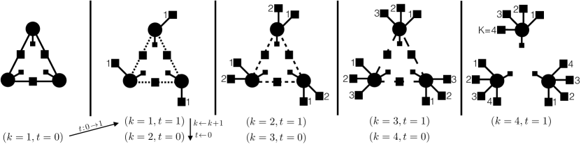
Figure 1: Factor graph representation of the $(k,t)$–interpolating model $P_{k,t;\epsilon=0}({\mathbf{x}}|\bm{\theta})$ for $k=1,\ldots,K=4$. The adaptive interpolation is parametrized by two distinct “time” parameters: A discrete one $k=1,\ldots,K$ that controls the interpolation at a global level. Then for a fixed $k$ we define a continuous $t\in[0,1]$ that controls the interpolation at a local level. The adaptive interpolation iteratively “constructs” the mean-field (decoupled) model, corresponding to $(k=K,t=1)$, by starting from the original model $(k=1,t=0)$ and then incrementally reducing the interaction strength of the edges associated with the original model, while compensating by adding mean-field decoupled factors to the graph (the small factors acting independently on each nodes that represent the factorized prior $P_{0}$ remain unchanged). This works as follows. At a fixed discrete step $k$, letting $t$ increase from $0$ to $1$ continuously decreases the strength of all the interactions of the original model by a factor $K^{-1}$, while continuously adding the $k$-th Gaussian mean-field factors (one equivalent factor per node). This corresponds to the local interpolation. Then $k$ is increased by one unit, $t$ is set to $0$ and the local interpolation process is then repeated. At the end of the adaptive interpolation, the set of all interactions of the original model have been replaced by $K$ Gaussian mean-fields per node. An important matching property is that the $(k,t=1)$ and $(k+1,t=0)$ models are statistically equivalent.

Let ${\mathbf{z}}^{(k)}=[z_{ij}^{(k)}]_{i,j=1}^{n},\widetilde{{\mathbf{z}}}^{(k)}=[\widetilde{z_{i}}^{(k)}]_{i=1}^{n}$, $Z_{ij}^{(k)}=Z_{ji}^{(k)}\sim{\cal N}(0,1)$, $\widetilde{Z}_{i}^{(k)}\sim{\cal N}(0,1)$ for $k=1,\ldots,K$ be Gaussian noise symmetric matrices and vectors. It is important to keep in mind that these are indexed both by the vertex indices $i,j$ and the discrete global interpolation parameter $k$.

The $(k,t)$–interpolating Hamiltonian is

$${\cal H}_{k,t}({\mathbf{x}})\vcentcolon= \sum_{k^{\prime}=k+1}^{K}h\Big{(}{\mathbf{x}},{\mathbf{s}},{\mathbf{z}}^{(k^{\prime})},K\Delta\Big{)}+\sum_{k^{\prime}=1}^{k-1}h_{\rm mf}\Big{(}{\mathbf{x}},{\mathbf{s}},\widetilde{{\mathbf{z}}}^{(k^{\prime})},\frac{K\Delta}{m_{k^{\prime}}}\Big{)}$$

$$\qquad+h\Big{(}{\mathbf{x}},{\mathbf{s}},{\mathbf{z}}^{(k)},\frac{K\Delta}{1-t}\Big{)}+h_{\rm mf}\Big{(}{\mathbf{x}},{\mathbf{s}},\widetilde{{\mathbf{z}}}^{(k)},\frac{K\Delta}{t\,m_{k}}\Big{)},$$ (14)

where the trial parameters $\{m_{k}\}_{k=1}^{K}$ are to be fixed later (these will be chosen ${\cal O}(1)$ with respect to (w.r.t) $n$ and can be interpreted as signal-to-noise ratios), $t\in[0,1]$ the continuous local interpolation parameter, and

$$h({\mathbf{x}},{\mathbf{s}},{\mathbf{z}},\sigma^{2}) \vcentcolon=\frac{1}{\sigma^{2}}\sum_{i\leq j=1}^{n}\Big{(}\frac{x_{i}^{2}x_{j}^{2}}{2n}-\frac{x_{i}x_{j}s_{i}s_{j}}{n}-\frac{\sigma x_{i}x_{j}z_{ij}}{\sqrt{n}}\Big{)},$$ (15)

$$h_{\rm mf}({\mathbf{x}},{\mathbf{s}},\widetilde{{\mathbf{z}}},\sigma^{2}) \vcentcolon=\frac{1}{\sigma^{2}}\sum_{i=1}^{n}\Big{(}\frac{x_{i}^{2}}{2}-x_{i}s_{i}-\sigma x_{i}\widetilde{z}_{i}\Big{)}.$$ (16)

Here the subscript “mf” stands for “mean-field”.

A possible interpretation of the scheme is the following. The $(k,t)$–interpolating model corresponds to the following inference model. One has access to the following sets of noisy observations about the signal ${\mathbf{s}}$ where each noise realization is independent:

$$\Big{\{} {\mathbf{w}}^{(k^{\prime})}=\frac{{\mathbf{s}}{\mathbf{s}}^{\intercal}}{\sqrt{n}}+{\mathbf{z}}^{(k^{\prime})}\sqrt{K\Delta}\Big{\}}_{k^{\prime}=k+1}^{K},$$ (17)

$$\Big{\{} {\mathbf{y}}^{(k^{\prime})}={\mathbf{s}}+\widetilde{\mathbf{z}}^{(k^{\prime})}\sqrt{\frac{K\Delta}{m_{k^{\prime}}}}\Big{\}}_{k^{\prime}=1}^{k-1},$$ (18)

$${\mathbf{w}}^{(k)}=\frac{{\mathbf{s}}{\mathbf{s}}^{\intercal}}{\sqrt{n}}+{\mathbf{z}}^{(k)}\sqrt{\frac{K\Delta}{1-t}},$$ (19)

$${\mathbf{y}}^{(k)}={\mathbf{s}}+\widetilde{\mathbf{z}}^{(k)}\sqrt{\frac{K\Delta}{t\,m_{k}}}.$$ (20)

The first and third sets of observations correspond to similar inference channels as the original model (1) but with a much higher noise variance proportional to $K$. These correspond to the first and third terms, respectively, of the $(k,t)$–interpolating Hamiltonian (2.2). The second and fourth sets instead correspond to decoupled Gaussian denoising models, with associated “mean-field” second and fourth terms in (2.2). The noise variances are proportional to $K$ because the total number of observations is $K$ and we want the total signal-to-noise ratio to be ${\cal O}(1)$. At fixed $k$, letting $t$ increase from $0$ to $1$ increases by one unit the number of decoupled observations (18) by continuously adding the observation (20): Its signal-to-noise ratio that vanishes at $t=0$ (which is equivalent to not having access to this observation) becomes finite and equal to the signal-to-noise ratio of the individual observations in the set (18) at $t=1$. Simultaneously it reduces by one the number of observations of the form (17) by “removing” the observation (19): its signal-to-noise ratio, which is finite at $t=0$, vanishes at $t=1$. From (17)–(20) it is clear that the $(k,t=1)$ and $(k+1,t=0)$–interpolating models are statistically equivalent. A complementary and more graphical illustration of the interpolation scheme is found on Figure 1.

In order to use an important concentration lemma later on, we will need a slightly more general Hamiltonian, and consider the following perturbed version of (2.2):

$${\cal H}_{k,t;\epsilon}({\mathbf{x}};\bm{\theta})\vcentcolon={\cal H}_{k,t}({\mathbf{x}})+\epsilon\sum_{i=1}^{n}\Big{(}\frac{x_{i}^{2}}{2}-x_{i}s_{i}-\frac{x_{i}\widehat{z}_{i}}{\sqrt{\epsilon}}\Big{)},$$ (21)

with i.i.d $\widehat{Z}_{i}\sim{\cal N}(0,1)$ and $\bm{\Theta}\vcentcolon=\{{\mathbf{S}},\{{\mathbf{Z}}^{(k)},\widetilde{{\mathbf{Z}}}^{(k)}\}_{k=1}^{K},\widehat{\mathbf{Z}}\}$ is the collection of all quenched random variables. It should be kept in mind that the signal-to-noise ratio $\epsilon$ of this additional Gaussian “side-channel” ${\mathbf{y}}={\mathbf{s}}\sqrt{\epsilon}+\widehat{\mathbf{z}}$ will tend to $0$ at the end of the proof. Therefore we always consider $\epsilon\in[0,1]$.

The $(k,t)$–interpolating model has an associated posterior distribution, Gibbs expectation $\langle-\rangle_{k,t;\epsilon}$ and $(k,t)$–interpolating free energy $f_{k,t;\epsilon}$:

$$P_{k,t;\epsilon}({\mathbf{x}}|\bm{\theta}) \vcentcolon=\frac{\prod_{i=1}^{n}P_{0}(x_{i})e^{-{\cal H}_{k,t;\epsilon}({\mathbf{x}};\bm{\theta})}}{\int\bigl{\{}\prod_{i=1}^{n}dx_{i}P_{0}(x_{i})\bigr{\}}e^{-{\cal H}_{k,t;\epsilon}({\mathbf{x}};\bm{\theta})}},$$ (22)

$$\langle A({\mathbf{X}})\rangle_{k,t;\epsilon} \vcentcolon=\int d{\mathbf{x}}\,A({\mathbf{x}})P_{k,t;\epsilon}({\mathbf{x}}|\bm{\theta}),$$ (23)

$$f_{k,t;\epsilon} \vcentcolon=-\frac{1}{n}\mathbb{E}_{\bm{\Theta}}\Big{[}\ln\int\big{\{}\prod_{i=1}^{n}dx_{i}P_{0}(x_{i})\big{\}}e^{-{\cal H}_{k,t;\epsilon}({\mathbf{x}};\bm{\Theta})}\Big{]}.$$ (24)

In the following, we simply denote $\mathbb{E}_{\bm{\Theta}}$ by $\mathbb{E}$.

Lemma 1 (Linking the perturbed and plain free energies).

Let $P_{0}$ have finite second moment. Then for the initial and final systems

$$|f_{1,0;\epsilon}-f_{1,0;0}|\leq\frac{\epsilon}{2}\mathbb{E}[S^{2}]\,,\quad\text{and}\quad|f_{K,1;\epsilon}-f_{K,1;0}|\leq\frac{\epsilon}{2}\mathbb{E}[S^{2}]\,.$$ (25)

A short and generic proof is found in Appendix A. This statement shows in particular that if the thermodynamic limit $n\to+\infty$ exists, then it can be exchanged with the limit $\epsilon\to 0_{+}$ (as long as $P_{0}$ has bounded second moment). We stress that the existence of the thermodynamic limit is not directly used in our subsequent analysis, but rather, follows as a consequence.

2.3 The initial and final models

Let us compute the $(k,t)$–interpolating free energy $f_{1,0;0}$ associated with the initial $(k=1,t=0)$ model. Using (2.2) and (15),

$${\cal H}_{1,0;0}({\mathbf{x}};\bm{\theta})= \sum_{k=1}^{K}h\Big{(}{\mathbf{x}},{\mathbf{s}},{\mathbf{z}}^{(k)},K\Delta\Big{)}=\frac{1}{\Delta}\sum_{i\leq j=1}^{n}\Big{(}\frac{x_{i}^{2}x_{j}^{2}}{2n}-\frac{x_{i}x_{j}s_{i}s_{j}}{n}-\frac{x_{i}x_{j}}{\sqrt{n}}\sqrt{\Delta}\sum_{k=1}^{K}\frac{z_{ij}^{(k)}}{\sqrt{K}}\Big{)}.$$ (26)

As the $Z_{ij}^{(k)}$, $1\leq i\leq j\leq n$, are i.i.d ${\cal N}(0,1)$ random variables, they possess the stability property, namely $Z_{ij}\vcentcolon=\sum_{k=1}^{K}Z_{ij}^{(k)}/\sqrt{K}$ are i.i.d ${\cal N}(0,1)$ random variables as well (and symmetric). Let ${\mathbf{z}}=[z_{ij}]_{i,j=1}^{n}$. Using this we obtain

$$f_{1,0;0}=-\frac{1}{n}\mathbb{E}_{{\mathbf{S}},{\mathbf{Z}}}\Big{[}\ln\int\big{\{}\prod_{i=1}^{n}dx_{i}P_{0}(x_{i})\big{\}}e^{-{\cal H}_{1,0;0}({\mathbf{x}};{\mathbf{S}},{\mathbf{Z}})}\Big{]}$$ (27)

which is actually the free energy (7) of the original model. We thus have:

$$f_{1,0;0}=f_{n}.$$ (28)

Let us now consider the free energy $f_{K,1;0}$ of the final model. Using (2.2) and (16) we get

$${\cal H}_{K,1;0}({\mathbf{x}};\bm{\theta})= \sum_{k=1}^{K}h_{\rm mf}\Big{(}{\mathbf{x}},{\mathbf{s}},\widetilde{{\mathbf{z}}}^{(k)},\frac{K\Delta}{m_{k}}\Big{)}=\sum_{k=1}^{K}\frac{m_{k}}{K\Delta}\sum_{i=1}^{n}\Big{(}\frac{x_{i}^{2}}{2}-x_{i}s_{i}-x_{i}\widetilde{z}_{i}^{(k)}\sqrt{\frac{K\Delta}{m_{k}}}\Big{)}.$$ (29)

Define

$$m_{\rm mf}^{(K)}\vcentcolon=\frac{1}{K}\sum_{k=1}^{K}m_{k}.$$ (30)

Simple algebra leads to

$${\cal H}_{K,1;0}({\mathbf{x}};\bm{\theta})=\frac{m_{\rm mf}^{(K)}}{\Delta}\sum_{i=1}^{n}\Big{(}\frac{x_{i}^{2}}{2}-x_{i}s_{i}-x_{i}\sqrt{\frac{\Delta}{m_{\rm mf}^{(K)}}}\sum_{k=1}^{K}\widetilde{z}_{i}^{(k)}\sqrt{\frac{m_{k}}{Km_{\rm mf}^{(K)}}}\Big{)}.$$ (31)

We now proceed as previously using again the stability property of the Gaussian noise variables. Since $\widetilde{Z}_{i}^{(k)}$ are i.i.d ${\cal N}(0,1)$, then $\widetilde{Z}_{i}\vcentcolon=\sum_{k=1}^{K}\widetilde{Z}_{i}^{(k)}\sqrt{m_{k}/(Km_{\rm mf}^{(K)})}\sim{\cal N}(0,1)$ and are i.i.d. Let $\widetilde{\mathbf{z}}=[\widetilde{z}_{i}]_{i=1}^{n}$. Using (24) we find that $f_{K,1;0}$ can also be expressed as

$$f_{K,1;0} =-\frac{1}{n}\mathbb{E}_{{\mathbf{S}},\widetilde{\mathbf{Z}}}\Big{[}\ln\int\big{\{}\prod_{i=1}^{n}dx_{i}P_{0}(x_{i})\big{\}}\exp\Big{\{}-\frac{m_{\rm mf}^{(K)}}{\Delta}\sum_{i=1}^{n}\big{(}\frac{x_{i}^{2}}{2}-x_{i}S_{i}-x_{i}\widetilde{Z}_{i}\sqrt{\frac{\Delta}{m_{\rm mf}^{(K)}}}\big{)}\Big{\}}\Big{]}$$

$$=-\mathbb{E}_{S,\widetilde{Z}}\Big{[}\ln\int dxP_{0}(x)\exp\Big{\{}-\frac{m_{\rm mf}^{(K)}}{\Delta}\big{(}\frac{x^{2}}{2}-xS-x\widetilde{Z}\sqrt{\frac{\Delta}{m_{\rm mf}^{(K)}}}\big{)}\Big{\}}\Big{]}.$$ (32)

Expression (32) is nothing else than the free energy (10) associated with the following scalar denoising model: $y=s+\widetilde{z}\,\Sigma(m_{\rm mf}^{(K)};\Delta)$, which leads to

$$f_{K,1;0}=f_{\rm den}\big{(}\Sigma(m_{\rm mf}^{(K)};\Delta)\big{)}.$$ (33)

2.4 Free energy change along the adaptive interpolation path

By construction of (2.2) we have the following coherency property (see Figure 1): The $(k,t=1)$ and $(k+1,t=0)$ models are equivalent (the Hamiltonian (2.2) is invariant under this change) and thus $f_{k,1;\epsilon}=f_{k+1,0;\epsilon}$ for any $k$. This implies that the $(k,t)$–interpolating free energy (24) verifies

$$f_{1,0;\epsilon}=f_{K,1;\epsilon}+\sum_{k=1}^{K}(f_{k,0;\epsilon}-f_{k,1;\epsilon})=f_{K,1;\epsilon}-\sum_{k=1}^{K}\int_{0}^{1}dt\frac{df_{k,t;\epsilon}}{dt}.$$ (34)

Let us evaluate $df_{k,t;\epsilon}/dt$. Define the overlap $q_{{\mathbf{x}},{\mathbf{s}}}\vcentcolon=n^{-1}\sum_{i=1}^{n}x_{i}s_{i}$. Starting from (24), lenghty but simple algebra (see sec. 2.7 for the details) shows that as long as $P_{0}$ has bounded first four moments,

$$\frac{df_{k,t;\epsilon}}{dt}=\frac{1}{4\Delta K}\mathbb{E}[\langle q_{{\mathbf{X}},{\mathbf{S}}}^{2}-2m_{k}q_{{\mathbf{X}},{\mathbf{S}}}\rangle_{k,t;\epsilon}]+{\cal O}((nK)^{-1}).$$ (35)

This, with (34) and (33) yields

$$f_{1,0;\epsilon} =f_{K,1;\epsilon}-\frac{1}{4\Delta K}\sum_{k=1}^{K}\int_{0}^{1}dt\,\mathbb{E}[\langle q_{{\mathbf{X}},{\mathbf{S}}}^{2}-2m_{k}q_{{\mathbf{X}},{\mathbf{S}}}\rangle_{k,t;\epsilon}]+{\cal O}(n^{-1})$$

$$=(f_{K,1;\epsilon}-f_{K,1;0})+f_{\rm den}\big{(}\Sigma(m_{\rm mf}^{(K)};\Delta)\big{)}$$

$$\qquad-\frac{1}{4\Delta}\Big{\{}-\frac{1}{K}\sum_{k=1}^{K}m_{k}^{2}+\frac{1}{K}\sum_{k=1}^{K}\int_{0}^{1}dt\,\mathbb{E}[\langle(q_{{\mathbf{X}},{\mathbf{S}}}-m_{k})^{2}\rangle_{k,t;\epsilon}]\Big{\}}+{\cal O}(n^{-1})$$

$$=(f_{K,1;\epsilon}-f_{K,1;0})+f_{\rm RS}(m_{\rm mf}^{(K)};\Delta)+\frac{V_{K}(\{m_{k}\}_{k=1}^{K})}{4\Delta}$$

$$\qquad-\frac{1}{4\Delta K}\sum_{k=1}^{K}\int_{0}^{1}dt\,\mathbb{E}[\langle(q_{{\mathbf{X}},{\mathbf{S}}}-m_{k})^{2}\rangle_{k,t;\epsilon}]+{\cal O}(n^{-1}),$$ (36)

where in the last equality we used (8) and introduced the non-negative variance

$$V_{K}(\{m_{k}\}_{k=1}^{K})\vcentcolon=\frac{1}{K}\sum_{k=1}^{K}m_{k}^{2}-\Big{(}\frac{1}{K}\sum_{k=1}^{K}m_{k}\Big{)}^{2}.$$ (37)

The fundamental sum rule (36) can now be used to prove the replica symmetric formula.

2.5 Upper bound

From (36) we recover the upper bound usually obtained by the classical method of Guerra and Toninelli [50] and applied in [21] to symmetric rank-one matrix estimation (but see also [20] which already fully proved the replica formula in the binary case). Choose $m_{k}={\rm argmin}_{m\geq 0}f_{\rm RS}(m;\Delta)$ for all $k=1,\ldots,K$. This implies $m_{\rm mf}^{(K)}={\rm argmin}_{m\geq 0}f_{\rm RS}(m;\Delta)$ as well as $V_{K}(\{m_{k}\})=0$. Thus since the integrand in (36) is non-negative we get the bound

$$f_{1,0;\epsilon}\leq(f_{K,1;\epsilon}-f_{K,1;0})+\min_{m\geq 0}f_{\rm RS}(m;\Delta)+{\cal O}(n^{-1}).$$ (38)

Now we apply this inequality to a sequence $\epsilon_{n}\to 0$ as $n\to+\infty$. From Lemma 1 and (28) we obtain the upper bound:

Proposition 1 (Upper bound).

Fix $\Delta>0$. For any $P_{0}$ with bounded first four moments,

$$\limsup_{n\to\infty}f_{n}\leq\min_{m\geq 0}f_{\rm RS}(m;\Delta).$$ (39)

2.6 Lower bound

The converse bound is generally the one requiring extra technical tools, such as the use of spatial coupling [51, 28, 22, 17, 18] or the Aizenman-Sims-Starr scheme, see [35, 33, 32, 31]. Thanks to the adaptive interpolation method the proof is quite straightforward. As in all of the existing methods, we need a concentration lemma which takes the following form in the present context (see sec. 5 for the proof).

Lemma 2 (Overlap concentration).

Let $P_{0}$ have bounded support. For any sequences $K_{n}\to+\infty$, $0<a_{n}<b_{n}<1$, and any choice of the trial parameters $m_{k}:\epsilon\mapsto m_{k}^{(n)}(\epsilon)$, $k=1,\cdots,K$ differentiable, bounded, non-decreasing with respect to $\epsilon$, we have

$$\int_{a_{n}}^{b_{n}}d\epsilon\,\frac{1}{K_{n}}\sum_{k=1}^{K_{n}}\int_{0}^{1}dt\,\mathbb{E}\big{[}\big{\langle}(q_{{\mathbf{X}},{\mathbf{S}}}-\mathbb{E}[\langle q_{{\mathbf{X}},{\mathbf{S}}}\rangle_{k,t;\epsilon}])^{2}\big{\rangle}_{k,t;\epsilon}\big{]}\leq\frac{C}{a_{n}^{2}n^{\alpha}},$$ (40)

for any $0<\alpha<1/4$ and some constant $C>0$ independent of $n$, $K_{n}$, $b_{n}$ and the set of trial parameters ($C$ depends on the second moment and the support of $P_{0}$).

Remark 3.

In applications of this lemma the sequence $a_{n}$ tends to zero as slowly as we wish. In practice we will set later on $b_{n}=2a_{n}$ and take $a_{n}\to 0$ slowly enough so that $a_{n}^{-3}n^{-\alpha}\to 0$. In particular the r.h.s of (40) tends to zero.

For sequences $K_{n}$, $0<a_{n}<b_{n}<1$, and $\{m_{k}=m_{k}^{(n)}(\epsilon)\}_{k=1}^{K}$ as in Lemma 2, (36) becomes

$$\int_{a_{n}}^{b_{n}}d\epsilon\,f_{1,0;\epsilon} =\int_{a_{n}}^{b_{n}}d\epsilon\,(f_{K_{n},1;\epsilon}-f_{K_{n},1;0})+\int_{a_{n}}^{b_{n}}d\epsilon\,\biggl{\{}f_{\rm RS}(m_{\rm mf}^{(K_{n})};\Delta)+\frac{V_{K_{n}}(\{m_{k}\}_{k=1}^{K_{n}})}{4\Delta}\biggr{\}}$$

$$\qquad-\frac{1}{4\Delta}\int_{a_{n}}^{b_{n}}d\epsilon\,\frac{1}{K_{n}}\sum_{k=1}^{K_{n}}\int_{0}^{1}dt\,\big{(}\mathbb{E}[\langle q_{{\mathbf{X}},{\mathbf{S}}}\rangle_{k,t;\epsilon}]-m_{k}\big{)}^{2}+\mathcal{O}(a_{n}^{-2}n^{-\alpha})$$ (41)

where ${\cal O}(a_{n}^{-2}n^{-\alpha})$ is uniform in the choice of $K_{n}$, $b_{n}$ and trial parameters. At this point we need another important Lemma (see Appendix B for the proof) which is made possible by construction of the adaptive interpolation method.

Lemma 3 (Weak $t$-dependence at fixed $k$).

Fix $K$, $\epsilon$ and $\{m_{k}\}_{k=1}^{K}$. For $P_{0}$ with bounded first four moments and any $k\in\{1,\ldots,K\}$ and $t\in[0,1]$,

$$\big{|}\mathbb{E}[\langle q_{{\mathbf{X}},{\mathbf{S}}}\rangle_{k,t;\epsilon}]-\mathbb{E}[\langle q_{{\mathbf{X}},{\mathbf{S}}}\rangle_{k,0;\epsilon}]\big{|}={\cal O}\Big{(}\frac{n}{K}\Big{)}.$$ (42)

uniformly in $\epsilon$ and $\{m_{k}\}_{k=1}^{K}$. This result also applies when fixed $K$ is replaced by $K_{n}$ and $\{m_{k}=m_{k}^{(n)}(\epsilon)\}$.

Using this lemma for a sequence $K_{n}=\Omega(n^{b})$ with $b>1$ large enough, say $b=2$, (2.6) takes the following convenient form:

$$\int_{a_{n}}^{b_{n}}d\epsilon\,f_{1,0;\epsilon}= \,\int_{a_{n}}^{b_{n}}d\epsilon\,(f_{K_{n},1;\epsilon}-f_{K_{n},1;0})+\int_{a_{n}}^{b_{n}}d\epsilon\,\biggl{\{}f_{\rm RS}(m_{\rm mf}^{(K_{n})};\Delta)+\frac{V_{K_{n}}(\{m_{k}\}_{k=1}^{K_{n}})}{4\Delta}\biggr{\}}$$

$$\qquad-\frac{1}{4\Delta}\int_{a_{n}}^{b_{n}}d\epsilon\,\frac{1}{K_{n}}\sum_{k=1}^{K_{n}}\big{(}\mathbb{E}[\langle q_{{\mathbf{X}},{\mathbf{S}}}\rangle_{k,0;\epsilon}]-m_{k}\big{)}^{2}+\mathcal{O}(a_{n}^{-2}n^{-\alpha}).$$ (43)

We now use the last crucial lemma which is a fundamental property of the adaptive interpolation.

Lemma 4 (Choice for the trial parameters).

For a given $n$ one can freely select differentiable and non-decreasing trial parameters $\{m_{k}=m_{k}^{(n)}(\epsilon)\}_{k=1}^{K}$ as

$$m_{k}=\mathbb{E}[\langle q_{{\mathbf{X}},{\mathbf{S}}}\rangle_{k,0;\epsilon}],\quad k=1,\cdots,K_{n}.$$ (44)

Proof.

This is authorized by construction of the adaptive interpolation method. Indeed, the $(k=1,t=0)$–interpolating model (see the Hamiltonian ${\cal H}_{1,0;\epsilon}({\mathbf{x}};\bm{\theta})$ in (2.2)) is independent of $\{m_{k}\}_{k=1}^{K_{n}}$. Thus we can freely set $m_{1}=m_{1}^{(n)}(\epsilon)=\mathbb{E}[\langle q_{{\mathbf{X}},{\mathbf{S}}}\rangle_{1,0;\epsilon}]$. Once $m_{1}$ is fixed to this value $m_{1}^{(n)}(\epsilon)$, we go to the next step and set $m_{2}=m_{2}^{(n)}(\epsilon)=\mathbb{E}[\langle q_{{\mathbf{X}},{\mathbf{S}}}\rangle_{2,0;\epsilon}]$, which again is possible due to the fact that the Hamiltonian ${\cal H}_{2,0;\epsilon}({\mathbf{x}};\bm{\theta})$ and the Gibbs average $\langle-\rangle_{2,0;\epsilon}$ as well depend only on $m_{1}$ which has already been fixed. And so forth: As seen from Fig. 1, the Gibbs average $\langle-\rangle_{k,0;\epsilon}$ depends only on $\{m_{k^{\prime}}\}_{k^{\prime}=1}^{k-1}$ which were already fixed in the previous steps so that the choice (44) is valid. Note that $\mathbb{E}[\langle q_{{\mathbf{X}},{\mathbf{S}}}\rangle_{k,0;\epsilon}]\geq 0$ which is important as the $m_{k}^{(n)}(\epsilon)$’s play the role of signal-to-noise ratios, and thus must be positive. Moreover the maps $\epsilon\mapsto m_{k}^{(n)}(\epsilon)$ are differentiable and non-decreasing. They are obviously differentiable since we work with $n$ finite. To see that they are non-decreasing we look at their derivative. It is easy to see from the construction of the Gibbs bracket that $\mathbb{E}[\langle q_{{\mathbf{X}},{\mathbf{S}}}\rangle_{k,0;\epsilon}]$ is a function $\epsilon\mapsto G_{k}^{(n)}(\epsilon+\frac{1}{K}\sum_{l=1}^{k-1}m_{l})$ so that

$$\frac{d}{d\epsilon}m_{k}^{(n)}(\epsilon)=G_{k}^{(n)\prime}\biggl{(}\epsilon+\frac{1}{K}\sum_{l=1}^{k-1}m_{l}^{(n)}(\epsilon)\biggr{)}\biggl{(}1+\frac{1}{K}\sum_{l=1}^{k-1}\frac{d}{d\epsilon}m_{l}^{(n)}(\epsilon)\biggr{)}\,.$$

Now, $G_{k}^{(n)\prime}$ is an expected variance, and is therefore positive, as can be directly shown from a direct calculation (see equations (118) and (119) in section 5). This implies by induction that $\frac{d}{d\epsilon}m_{k}^{(n)}(\epsilon)\geq 0$. ∎

With this particular choice of trial parameters $\{m_{k}=m_{k}^{(n)}(\epsilon)\}_{k=1}^{K_{n}}$ the sum over $k=1,\ldots,K_{n}$ in (2.6) is set to zero: The interpolation path has been adapted (thus the name of the method). Since $V_{K_{n}}$ is non-negative, (2.6) directly implies the following lower bound:

$$\int_{a_{n}}^{b_{n}}d\epsilon\,f_{1,0;\epsilon} =\int_{a_{n}}^{b_{n}}d\epsilon\,\biggl{\{}(f_{K_{n},1;\epsilon}-f_{K_{n},1;0})+f_{\rm RS}\Big{(}K_{n}^{-1}\sum_{k=1}^{K_{n}}m_{k}^{(n)};\Delta\Big{)}+\frac{V_{K_{n}}(\{m_{k}^{(n)}\}_{k=1}^{K_{n}})}{4\Delta}\biggr{\}}+\mathcal{O}(a_{n}^{-2}n^{-\alpha})$$

$$\geq\int_{a_{n}}^{b_{n}}d\epsilon\,(f_{K_{n},1;\epsilon}-f_{K_{n},1;0})+(b_{n}-a_{n})\min_{m\geq 0}f_{\rm RS}(m;\Delta)+\mathcal{O}(a_{n}^{-2}n^{-\alpha}).$$ (45)

Finally, setting $b_{n}=2a_{n}$ and taking $a_{n}\to 0$ slowly enough as $n\to+\infty$ so that $a_{n}^{-3}n^{-\alpha}\to 0$, using Lemma 1 and (28) and the mean value theorem, we deduce

Proposition 2 (Lower bound).

Fix $\Delta>0$. For any $P_{0}$ with bounded support,

$$\liminf_{n\to\infty}f_{n}\geq\min_{m\geq 0}f_{\rm RS}(m;\Delta).$$ (46)

Remark 4 (The overlap must concentrate).

Note that it is not obvious that one can find $\{m_{k}^{(n)}(\epsilon)\}_{k=1}^{K_{n}}$ which directly cancel the integrals in the fundamental identity (36) without using the overlap concentration of Lemma 2. Overlap concentration is a fundamental requirement of the above proof. This agrees with the statistical physics assumption that a necessary condition for the validity of the replica symmetric method is precisely the overlap concentration [5].

In Appendix C we present an alternative useful, albeit not completely rigorous, argument to obtain the lower bound.

2.7 Proof of the fundamental sum rule

In this paragraph we derive the formula (35). We will need a simple but fundamental identity which is a straightforward consequence of the Bayes law. Let ${\mathbf{X}}$, ${\mathbf{X}}^{\prime}$ be two i.i.d “replicas” drawn according to the product distribution $P_{k,t;\epsilon}({\mathbf{x}}|\bm{\theta})P_{k,t;\epsilon}({\mathbf{x}}^{\prime}|\bm{\theta})$. Recall the notation $\bm{\theta}\vcentcolon=\{{\mathbf{s}},\{{\mathbf{z}}^{(k)},\widetilde{{\mathbf{z}}}^{(k)}\}_{k=1}^{K},\widehat{\mathbf{z}}\}$ for the quenched variables and $\mathbb{E}=\mathbb{E}_{\bm{\Theta}}$ for the expectation with respect to these. Then for any function $g$ which does not depend on the Gaussian noise random variables,

$$\mathbb{E}[\langle g({\mathbf{X}},{\mathbf{S}})\rangle_{k,t;\epsilon}]=\mathbb{E}[\langle g({\mathbf{X}},{\mathbf{X}}^{\prime})\rangle_{k,t;\epsilon}].$$ (47)

We give a proof of this identity in Appendix D for completeness.

Let us now compute $df_{k,t;\epsilon}/dt$. Starting from (2.2), (21), (24) one obtains

$$\frac{df_{k,t;\epsilon}}{dt} =\frac{1}{n}\mathbb{E}\Big{[}\Big{\langle}\frac{d{\cal H}_{k,t;\epsilon}({\mathbf{X}};\bm{\Theta})}{dt}\Big{\rangle}_{k,t;\epsilon}\Big{]}$$

$$=\frac{1}{n}\mathbb{E}\Big{[}\Big{\langle}\frac{d}{dt}h_{\rm mf}\Big{(}{\mathbf{x}},{\mathbf{s}},\widetilde{{\mathbf{z}}}^{(k)},\frac{K\Delta}{t\,m_{k}}\Big{)}+\frac{d}{dt}h\Big{(}{\mathbf{x}},{\mathbf{s}},{{\mathbf{z}}}^{(k)},\frac{K\Delta}{1-t}\Big{)}\Big{\rangle}_{k,t;\epsilon}\Big{]}$$

$$=\frac{1}{nK\Delta}\mathbb{E}\Big{[}\Big{\langle}m_{k}\sum_{i=1}^{n}\Big{(}\frac{X_{i}^{2}}{2}-X_{i}S_{i}-\frac{X_{i}\widetilde{Z}_{i}^{(k)}}{2}\sqrt{\frac{K\Delta}{t\,m_{k}}}\Big{)}$$

$$\qquad-\sum_{i\leq j=1}^{n}\Big{(}\frac{X_{i}^{2}X_{j}^{2}}{2n}-\frac{X_{i}X_{j}S_{i}S_{j}}{n}-\frac{X_{i}X_{j}Z_{ij}^{(k)}}{2\sqrt{n}}\sqrt{\frac{K\Delta}{1-t}}\Big{)}\Big{\rangle}_{k,t;\epsilon}\Big{]}.$$

Now we integrate by part the Gaussian noise using the elementary formula $\mathbb{E}_{Z}[Zf(Z)]=\mathbb{E}_{Z}[f^{\prime}(Z)]$ where $f^{\prime}$ is the derivative of $f$. This leads to

$$\frac{df_{k,t;\epsilon}}{dt} =\frac{1}{nK\Delta}\mathbb{E}\Big{[}\Big{\langle}m_{k}\sum_{i=1}^{n}\Big{(}\frac{X_{i}X_{i}^{\prime}}{2}-X_{i}S_{i}\Big{)}-\sum_{i\leq j=1}^{n}\Big{(}\frac{X_{i}X_{j}X_{i}^{\prime}X_{j}^{\prime}}{2n}-\frac{X_{i}X_{j}S_{i}S_{j}}{n}\Big{)}\Big{\rangle}_{k,t;\epsilon}\Big{]},$$ (48)

where ${\mathbf{X}}$, ${\mathbf{X}}^{\prime}$ are the two i.i.d replicas drawn according to (22). An application of identity (47) then leads to

$$\frac{df_{k,t;\epsilon}}{dt} =\frac{1}{2K\Delta}\mathbb{E}\Big{[}\Big{\langle}\frac{1}{n^{2}}\sum_{i\leq j=1}^{n}X_{i}X_{j}S_{i}S_{j}-\frac{m_{k}}{n}\sum_{i=1}^{n}X_{i}S_{i}\Big{\rangle}_{k,t;\epsilon}\Big{]}$$

$$=\frac{1}{2K\Delta}\mathbb{E}\Big{[}\Big{\langle}\frac{1}{2n^{2}}\sum_{i,j=1}^{n}X_{i}X_{j}S_{i}S_{j}+\frac{1}{2n^{2}}\sum_{i=1}^{n}X_{i}^{2}S_{i}^{2}-\frac{m_{k}}{n}\sum_{i=1}^{n}X_{i}S_{i}\Big{\rangle}_{k,t;\epsilon}\Big{]}.$$ (49)

The Cauchy-Schwarz inequality and (47) imply that $\mathbb{E}[\langle n^{-2}\sum_{i=1}^{n}X_{i}^{2}S_{i}^{2}\rangle_{k,t;\epsilon}]={\cal O}(n^{-1})$ as long as $P_{0}$ has bounded fourth moment. Indeed, by Cauchy-Schwarz

$$\mathbb{E}\Big{[}\Big{\langle}n^{-1}\sum_{i=1}^{n}X_{i}^{2}S_{i}^{2}\Big{\rangle}_{k,t;\epsilon}\Big{]}\leq\Big{(}\mathbb{E}\Big{[}\Big{\langle}n^{-1}\sum_{i=1}^{n}X_{i}^{4}\Big{\rangle}_{k,t;\epsilon}\Big{]}\Big{)}^{1/2}\Big{(}\mathbb{E}\Big{[}n^{-1}\sum_{i=1}^{n}S_{i}^{4}\Big{]}\Big{)}^{1/2}$$ (50)

and by (47) we have $\mathbb{E}[\langle X_{i}^{4}\rangle_{k,t;\epsilon}]=\mathbb{E}[S_{i}^{4}]$ for $i=1,\dots,n$, thus we get

$$\mathbb{E}\Big{[}\Big{\langle}n^{-1}\sum_{i=1}^{n}X_{i}^{2}S_{i}^{2}\Big{\rangle}_{k,t;\epsilon}\Big{]}\leq\mathbb{E}[S^{4}].$$ (51)

Finally, expressing the two other terms in (49) uisng the overlap $q_{{\mathbf{x}},{\mathbf{s}}}=n^{-1}\sum_{i=1}^{n}x_{i}s_{i}$ we find (35).

3  Application to rank-one symmetric tensor estimation

The present method can be extended to cover rank-one symmetric tensor estimation, which amounts to treat the $p$-spin model on the Nishimori line. For binary spins the Guerra-Toninelli bound was proven in [20] for any value of $p$, the replica symmetric formula was proved in the whole phase diagram for $p=2$, and also in a restricted region away from the first order phase transition for $p\geq 3$. A complete proof for $p=2$ and general spins (that can thus be real) was achieved using the spatial coupling technique in [22] and in [32] by a rigorous version of the cavity method. The case $p\geq 2$ and general spins has been treated using again the cavity method in [31].

3.1 Symmetric rank-one tensor estimation: Setting and main result

The symmetric tensor problem is very close to the matrix case presented in full details in sec. 2 so we only sketch the main steps. The observed symmetric tensor ${\mathbf{w}}\in\mathbb{R}^{n_{1}\times n_{2}\times\ldots\times n_{p}}$ is obtained through the following estimation model:

$$w_{i_{1}i_{2}\ldots i_{p}}=\sqrt{\frac{(p-1)!}{n^{p-1}}}s_{i_{1}}s_{i_{2}}\ldots s_{i_{p}}+z_{i_{1}i_{2}\ldots i_{p}}\sqrt{\Delta}\quad\text{for}\quad 1\leq i_{1}\leq i_{2}\leq\ldots\leq i_{p}\leq n,$$ (52)

where ${\mathbf{s}}\in\mathbb{R}^{n}$ with i.i.d components distributed according to a known prior $P_{0}$, ${\mathbf{Z}}\in\mathbb{R}^{n_{1}\times n_{2}\times\ldots\times n_{p}}$ is a symmetric Gaussian noise tensor with i.i.d (up to the symmetry constraint) ${\cal N}(0,1)$ entries. We note that, like in the case of symmetric matrix estimation of sec. 2.1, the channel universality property (see remark 2) is valid in the present setting. This means that by covering the case of additive white Gaussian noise (52), we actually treat a wide range of (component-wise) inference channels

$$P_{\rm out}(w_{i_{1}i_{2}\ldots i_{p}}|\sqrt{(p-1)!n^{1-p}}s_{i_{1}}s_{i_{2}}\ldots s_{i_{p}}).$$

We refer to [48, 53, 32] for more details on this point. The free energy of the model is

$$f_{n}\vcentcolon= -\frac{1}{n}\mathbb{E}_{{\mathbf{S}},{\mathbf{Z}}}\Big{[}\ln\int\big{\{}\prod_{i=1}^{n}dx_{i}P_{0}(x_{i})\big{\}}e^{-\mathcal{H}({\mathbf{x}};{\mathbf{S}},{\mathbf{Z}})}\Big{]}$$ (53)

where the Hamiltonian $\mathcal{H}({\mathbf{x}};{\mathbf{s}},{\mathbf{z}})$ is

$$\frac{1}{\Delta}\sum_{i_{1}\leq i_{2}\leq\ldots\leq i_{p}}\Big{(}\frac{(p-1)!}{2n^{p-1}}x_{i_{1}}^{2}\ldots x_{i_{p}}^{2}-\frac{(p-1)!}{n^{p-1}}x_{i_{1}}s_{i_{1}}\ldots x_{i_{p}}s_{i_{p}}-\sqrt{\frac{\Delta(p-1)!}{n^{p-1}}}z_{i_{1}i_{2}\ldots i_{p}}x_{i_{1}}\ldots x_{i_{p}}\Big{)}.$$ (54)

For a $P_{0}$ with bounded first four moments the free energy is related to the mutual information $I({\mathbf{S}};{\mathbf{W}})$ through

$$\frac{I({\mathbf{S}};{\mathbf{W}})}{n}=f_{n}+\frac{\mathbb{E}[S^{2}]^{p}}{2p\Delta}+{\cal O}(n^{-1}).$$ (55)

We define the replica symmetric potential for symmetric tensor estimation as

$$f_{\rm RS}(m;\Delta)\vcentcolon=\frac{(p-1)m^{p}}{2p\Delta}+f_{{\rm den}}\big{(}\Sigma(m;\Delta)\big{)}$$ (56)

where $\Sigma(m;\Delta)^{2}\vcentcolon=\Delta/m^{p-1}$ and $f_{{\rm den}}(\Sigma)$ is given by (10). Next we prove the RS formula.

Theorem 2 (RS formula for symmetric rank-one tensor estimation).

Fix $\Delta>0$. For any $P_{0}$ with bounded support, the asymptotic free energy of the symmetric tensor estimation model (52) verifies

$$\lim_{n\to\infty}f_{n}=\min_{m\geq 0}f_{\rm RS}(m;\Delta).$$ (57)

Again, we note that the bounded support property of $P_{0}$ is only needed for concentration proofs and does not impose any upper limit on the size of the support. We believe this can be removed by a limiting process as long as $P_{0}$ has bounded first four moments.

3.2 Sketch of proof of the replica symmetric formula

We prove Theorem 2. Since this proof is similar to the one of Theorem 1 for the matrix case, we only give the main ideas. The starting point is the introduction of a (perturbed) $(k,t)$–interpolating Hamiltonian:

$${\cal H}_{k,t;\epsilon}({\mathbf{x}};\bm{\theta}) \vcentcolon=\sum_{k^{\prime}=k+1}^{K}h\Big{(}{\mathbf{x}},{\mathbf{s}},{\mathbf{z}}^{(k^{\prime})},K\Delta\Big{)}+\sum_{k^{\prime}=1}^{k-1}h_{\rm mf}\Big{(}{\mathbf{x}},{\mathbf{s}},\widetilde{{\mathbf{z}}}^{(k^{\prime})},K\,\Sigma(m_{k};\Delta)^{2}\Big{)}$$

$$\quad+h\Big{(}{\mathbf{x}},{\mathbf{s}},{\mathbf{z}}^{(k)},\frac{K\Delta}{1-t}\Big{)}+h_{\rm mf}\Big{(}{\mathbf{x}},{\mathbf{s}},\widetilde{{\mathbf{z}}}^{(k)},\frac{K\,\Sigma(m_{k};\Delta)^{2}}{t}\Big{)}+\epsilon\sum_{i=1}^{n}\Big{(}\frac{x_{i}^{2}}{2}-x_{i}s_{i}-\frac{x_{i}\widehat{z}_{i}}{\sqrt{\epsilon}}\Big{)},$$ (58)

where the trial parameters $\{m_{k}\}_{k=1}^{K}$ are to be fixed later and

$$h({\mathbf{x}},{\mathbf{s}},{\mathbf{z}},\sigma^{2}) \vcentcolon=\frac{1}{\sigma^{2}}\sum_{i_{1}\leq i_{2}\leq\ldots\leq i_{p}}\Big{(}\frac{(p-1)!}{2n^{p-1}}x_{i_{1}}^{2}\ldots x_{i_{p}}^{2}-\frac{(p-1)!}{n^{p-1}}x_{i_{1}}s_{i_{1}}\ldots x_{i_{p}}s_{i_{p}}$$

$$\qquad\qquad-\sigma\sqrt{\frac{(p-1)!}{n^{p-1}}}z_{i_{1}i_{2}\ldots i_{p}}x_{i_{1}}\ldots x_{i_{p}}\Big{)},$$ (59)

$$h_{\rm mf}({\mathbf{x}},{\mathbf{s}},\widetilde{{\mathbf{z}}},\sigma^{2}) \vcentcolon=\frac{1}{\sigma^{2}}\sum_{i=1}^{n}\Big{(}\frac{x_{i}^{2}}{2}-x_{i}s_{i}-\sigma\widetilde{z}_{i}x_{i}\Big{)}.$$ (60)

The associated $(k,t)$–interpolating model, Gibbs expectation and $(k,t)$–interpolating free energy are defined respectively by (22), (23) and (24). Using the stability property of the Gaussian noise variables, one can check that the intial and final $(k,t)$–interpolating models are such that

$$f_{1,0;0} =f_{n},$$ (61)

$$f_{K,1;0} =f_{\rm den}\big{(}\Sigma_{\rm mf}(\{m_{k}\}_{k=1}^{K};\Delta)\big{)},$$ (62)

where

$$\Sigma_{\rm mf}(\{m_{k}\}_{k=1}^{K};\Delta)^{-2}\vcentcolon=\frac{1}{K}\sum_{k=1}^{K}\Sigma(m_{k};\Delta)^{-2}=\frac{1}{\Delta K}\sum_{k=1}^{K}m_{k}^{p-1}.$$ (63)

By a trivial generalization of the calculations of sec. 2.7, we obtain the variation of the $(k,t)$–interpolating free energy:

$$\frac{df_{k,t;\epsilon}}{dt}=\frac{1}{2p\Delta K}\mathbb{E}[\langle q_{{\mathbf{X}},{\mathbf{S}}}^{p}-p\,m_{k}^{p-1}q_{{\mathbf{X}},{\mathbf{S}}}\rangle_{k,t;\epsilon}]+{\cal O}((nK)^{-1}),$$ (64)

where the overlap is again $q_{{\mathbf{x}},{\mathbf{s}}}\vcentcolon=n^{-1}\sum_{i}^{n}x_{i}s_{i}$. This result holds as long as $P_{0}$ has finite first four moments. Proceeding similarly to section 2.4 we get the sum rule

$$f_{1,0;\epsilon} =(f_{K,1;\epsilon}-f_{K,1;0})+f_{\rm den}(\Sigma_{\rm mf}(\{m_{k}\}_{k=1}^{K};\Delta))+\frac{p-1}{2p\Delta K}\sum_{k=1}^{K}m_{k}^{p}$$

$$\qquad-\frac{1}{2p\Delta K}\sum_{k=1}^{K}\int_{0}^{1}dt\Big{(}\mathbb{E}[\langle q_{{\mathbf{X}},{\mathbf{S}}}^{p}\rangle_{k,t;\epsilon}]-p\,m_{k}^{p-1}\mathbb{E}[\langle q_{{\mathbf{X}},{\mathbf{S}}}\rangle_{k,t;\epsilon}]+(p-1)m_{k}^{p}\Big{)}+\mathcal{O}(n^{-1})$$

$$=(f_{K,1;\epsilon}-f_{K,1;0})+f_{\rm den}(\Sigma_{\rm mf}(\{m_{k}\}_{k=1}^{K};\Delta))+\frac{p-1}{2p\Delta^{-\frac{1}{p-1}}}\Big{(}\Sigma_{\rm mf}(\{m_{k}\}_{k=1}^{K};\Delta))^{-2}\Big{)}^{\frac{p}{p-1}}$$

$$\qquad+\frac{p-1}{2p\Delta}V_{K,p}(\{m_{k}\}_{k=1}^{K})$$

$$\qquad-\frac{1}{2p\Delta K}\sum_{k=1}^{K}\int_{0}^{1}dt\Big{(}\mathbb{E}[\langle q_{{\mathbf{X}},{\mathbf{S}}}^{p}\rangle_{k,t;\epsilon}]-p\,m_{k}^{p-1}\mathbb{E}[\langle q_{{\mathbf{X}},{\mathbf{S}}}\rangle_{k,t;\epsilon}]+(p-1)m_{k}^{p}\Big{)}+\mathcal{O}(n^{-1})$$ (65)

where

$$V_{K,p}(\{m_{k}\}_{k=1}^{K})\vcentcolon=\frac{1}{K}\sum_{k=1}^{K}m_{k}^{p}-\Big{(}\frac{1}{K}\sum_{k=1}^{K}m_{k}^{p-1}\Big{)}^{\frac{p}{p-1}}.$$ (66)

Note that $V_{K,p}$ is non-negative by Jensen’s inequality applied to the convex function $x\in\mathbb{R}_{+}\mapsto x^{\frac{p}{p-1}}\in\mathbb{R}_{+}$ (here the trial parameters are all non-negative). For $p=2$ the identity (65) reduces to (36).

The proof of Theorem 2 proceeds from this fundamental sum rule in much the same way as in the case $p=2$ of sections 2.5 and 2.6. Here we only give a brief summary of the arguments insisting only on the essential differences. We start with the upper bound.

For the case of even $p$ it is straightforward to derive an upper bound. One chooses all trial parameters as $m_{k}=m_{*}={\rm argmin}_{m\geq 0}f_{\rm RS}(m;\Delta)$, $k=1,\cdots,K$, which yields $V_{K,p}(\{m_{k}\}_{k=1}^{K})=0$. From there one can use the classic argument of Guerra-Toninelli: By convexity of $x\in\mathbb{R}\mapsto x^{p}\in\mathbb{R}_{+}$ for even $p$ we see that $q_{{\mathbf{X}},{\mathbf{S}}}^{p}-p\,m_{*}^{p-1}q_{{\mathbf{X}},{\mathbf{S}}}+(p-1)m_{*}^{p}\geq 0$, which implies the upper bound analogous to (38). Since Lemma 1 holds verbatim here, by taking a sequence $\epsilon_{n}\to 0_{+}$, $n\to+\infty$, we deduce as before the upper bound $\limsup_{n\to+\infty}f_{n}\leq\min_{m\geq 0}f_{\rm RS}(m;\Delta)$ (when $P_{0}$ has finite first four moments).

For the case of odd $p$ we cannot immediately apply the convexity argument. We first need to apply a concentration result. As it will become clear from its proof, Lemma 2 is generic and the same statement applies to the present tensor setting. Therefore for any sequence $K_{n}\to+\infty$, $0<a_{n}<b_{n}<1$, $b_{n}\to 0$, and trial parameters $\{m_{k}=m_{k}^{(n)}(\epsilon)\}_{k=1}^{K}$ which are non-decreasing functions of $\epsilon$ we have

$$\int_{a_{n}}^{b_{n}}d\epsilon\,f_{1,0;\epsilon}=\int_{a_{n}}^{b_{n}}d\epsilon\,(f_{K_{n},1;\epsilon}-f_{K_{n},1;0})+\int_{a_{n}}^{b_{n}}d\epsilon\,\biggl{\{}f_{\rm den}(\Sigma_{\rm mf}(\{m_{k}\}_{k=1}^{K_{n}};\Delta))$$

$$+\frac{p-1}{2p\Delta^{-\frac{1}{p-1}}}\Big{(}\Sigma_{\rm mf}(\{m_{k}\}_{k=1}^{K_{n}};\Delta))^{-2}\Big{)}^{\frac{p}{p-1}}+\frac{p-1}{2p\Delta}V_{K_{n},p}(\{m_{k}\}_{k=1}^{K_{n}})\biggr{\}}$$

$$-\frac{1}{2p\Delta}\int_{a_{n}}^{b_{n}}d\epsilon\,\frac{1}{K_{n}}\sum_{k=1}^{K_{n}}\int_{0}^{1}dt\Big{(}\mathbb{E}[\langle q_{{\mathbf{X}},{\mathbf{S}}}\rangle_{k,t;\epsilon}]^{p}-p\,m_{k}^{p-1}\mathbb{E}[\langle q_{{\mathbf{X}},{\mathbf{S}}}\rangle_{k,t;\epsilon}]+(p-1)m_{k}^{p}\Big{)}+\mathcal{O}(a_{n}^{-2}n^{-\alpha}),$$ (67)

for $0<\alpha<1/4$ and ${\cal O}(a_{n}^{-2}n^{-\alpha})$ uniform in $K_{n}$, $b_{n}$, and trial parameters. Furthermore by the Nishimori identity (47) we see that $\mathbb{E}[\langle q_{{\mathbf{X}},{\mathbf{S}}}\rangle_{k,t;\epsilon}]\geq 0$, so convexity of $x\in\mathbb{R}_{+}\mapsto x^{p}\in\mathbb{R}_{+}$ shows that the term under the integral is positive, which allows to deduce the upper bound as above (of course this argument works for any $p$ even or odd).

let us finally briefly discuss the lower bound. Lemma 3 and its proof hold for the tensor setting as well which means that in (67) we can replace $\mathbb{E}[\langle q_{{\mathbf{X}},{\mathbf{S}}}\rangle_{k,t;\epsilon}]$ by $\mathbb{E}[\langle q_{{\mathbf{X}},{\mathbf{S}}}\rangle_{k,0;\epsilon}]$. This then allows to choose (adapt) the sequence of trial parameters as $\{m_{k}=m_{k}^{(n)}(\epsilon)\}$ where $m_{k}=\mathbb{E}[\langle q_{{\mathbf{X}},{\mathbf{S}}}\rangle_{k,0;\epsilon}]$, $k=1,\cdots,K_{n}$ just as in Lemma 4. Thus we obtain

$$\int_{a_{n}}^{b_{n}}d\epsilon\,f_{1,0;\epsilon} =\int_{a_{n}}^{b_{n}}d\epsilon\,(f_{K_{n},1;\epsilon}-f_{K_{n},1;0})$$

$$\qquad+\int_{a_{n}}^{b_{n}}d\epsilon\,\biggl{\{}f_{\rm den}(\Sigma_{\rm mf}(\{m_{k}\}_{k=1}^{K_{n}};\Delta))+\frac{p-1}{2p\Delta^{-\frac{1}{p-1}}}\Big{(}\Sigma_{\rm mf}(\{m_{k}\}_{k=1}^{K_{n}};\Delta))^{-2}\Big{)}^{\frac{p}{p-1}}$$

$$\qquad+\frac{p-1}{2p\Delta}V_{K_{n},p}(\{m_{k}^{(n)}\}_{k=1}^{K_{n}})\biggr{\}}+\mathcal{O}(a_{n}^{-2}n^{-\alpha})$$

$$\geq\int_{a_{n}}^{b_{n}}d\epsilon\,(f_{K_{n},1;\epsilon}-f_{K_{n},1;0})+(b_{n}-a_{n})\min_{\Sigma\geq 0}\Big{\{}f_{\rm den}(\Sigma)+\frac{p-1}{2p\Delta^{-\frac{1}{p-1}}}\big{(}\Sigma^{-2}\big{)}^{\frac{p}{p-1}}\Big{\}}+\mathcal{O}(a_{n}^{-2}n^{-\alpha})$$

$$=\int_{a_{n}}^{b_{n}}d\epsilon\,(f_{K_{n},1;\epsilon}-f_{K_{n},1;0})+(b_{n}-a_{n})\min_{m\geq 0}f_{\rm RS}(m;\Delta)+\mathcal{O}(a_{n}^{-2}n^{-\alpha})$$ (68)

where we used the non-negativity of $V_{K,p}$ to get the inequality and the change of variable $\Sigma^{2}=\Delta/m^{p-1}$ to get the last line. The usual limiting argument, taking $b_{n}=2a_{n}$ with $a_{n}\to 0$ slowly enough so that $a_{n}^{-3}n^{-\alpha}\to 0$ when $n\to+\infty$, implies $\liminf_{n\to+\infty}f_{n}\geq\min_{m\geq 0}f_{\rm RS}(m;\Delta)$. We have proven this lower bound under the assumption of boundedness of the support of $P_{0}$ (used in the proof of overlap concentration)

Combining the upper and lower bounds yields Theorem 2. As a final note we remark that the alternative route to the lower bound proposed in Appendix C for the matrix case also holds essentially unchanged here.

4  Application to Gaussian random linear estimation

4.1 Gaussian random linear estimation: Setting and result

In Gaussian random linear estimation (RLE) one is interested in reconstructing a signal ${\mathbf{s}}=[s_{i}]_{i=1}^{n}\in\mathbb{R}^{n}$ from few noisy measurements ${\mathbf{y}}=[y_{\mu}]_{\mu=1}^{m}\in\mathbb{R}^{m}$ obtained from the projection of ${\mathbf{s}}$ by a random Gaussian measurement matrix $\bm{\phi}=[\phi_{\mu i}]_{\mu,i=1}^{m,n}\in\mathbb{R}^{m\times n}$ with i.i.d entries $\phi_{\mu i}\sim\mathcal{N}(0,1/n)$. The measurement rate is $\alpha\vcentcolon=m/n$. We consider i.i.d additive white Gaussian noise of known variance $\Delta$. Let the standardized noise components be $Z_{\mu}\sim\mathcal{N}(0,1)$, $\mu=1,\ldots,m$. Then the measurement model is

$${\mathbf{y}}=\bm{\phi}{{\mathbf{s}}}+{\mathbf{z}}\sqrt{\Delta},\qquad\text{or}\qquad y_{\mu}=\sum_{i=1}^{n}\phi_{\mu i}s_{i}+z_{\mu}\sqrt{\Delta}\quad\text{for}\quad 1\leq\mu\leq m.$$ (69)

The signal has i.i.d components distributed according to a discrete prior $P_{0}(s_{i})=\sum_{b=1}^{B}p_{b}\delta(s_{i}-a_{b})$ with a finite number $B$ of terms and $\max_{b}|a_{b}|\leq s_{\rm max}$. Note that the more general case where the signal has i.i.d vectorial components, as considered in [17, 18], can be tackled with our proof technique exactly in the same way but we consider the scalar case for the sake of notational simplicity.

The free energy of the RLE model (69) (which is also equal to the mutual information per component $I({\mathbf{S}};{\mathbf{Y}})/n$ between the noisy observation and the signal) is defined as

$$f_{n} \vcentcolon=-\frac{1}{n}\mathbb{E}_{{\mathbf{S}},{\mathbf{Z}},\bm{\Phi}}\Big{[}\ln\int\big{\{}\prod_{i=1}^{n}dx_{i}P_{0}(x_{i})\big{\}}\exp\Big{\{}-\frac{1}{\Delta}\sum_{\mu=1}^{m}\Big{(}\frac{1}{2}[\bm{\Phi}({\mathbf{x}}-{\mathbf{S}})]_{\mu}^{2}-[\bm{\Phi}({\mathbf{x}}-{\mathbf{S}})]_{\mu}Z_{\mu}\sqrt{\Delta}\Big{)}\Big{\}}\Big{]},$$ (70)

where $[\bm{\phi}({\mathbf{x}}-{\mathbf{s}})]_{\mu}\vcentcolon=\sum_{i=1}^{n}\bm{\phi}_{\mu i}(x_{i}-s_{i})$. Let

$$\Sigma(E;\Delta)^{-2} \vcentcolon=\frac{\alpha}{\Delta+E},$$ (71)

$$\psi(E;\Delta) \vcentcolon=\frac{\alpha}{2}\Big{(}\ln\Big{(}1+\frac{E}{\Delta}\Big{)}-\frac{E}{\Delta+E}\Big{)}.$$ (72)

Define the following RS potential:

$$f_{\rm RS}(E;\Delta)\vcentcolon=\psi(E;\Delta)+i_{\rm den}\big{(}\Sigma(E;\Delta)\big{)},$$ (73)

where $i_{\rm den}(\Sigma)=I(S;S+\widetilde{Z}\,\Sigma)$ is the mutual information of a scalar Gaussian denoising model $y=s+\widetilde{z}\,\Sigma$ with $S\sim P_{0}$, $\widetilde{Z}\sim{\cal N}(0,1)$, and $\Sigma^{-2}$ an effective signal to noise ratio:

$$i_{\rm den}(\Sigma)\vcentcolon=-\mathbb{E}_{S,\widetilde{Z}}\Big{[}\ln\int dxP_{0}(x)e^{-\frac{1}{\Sigma^{2}}\big{(}\frac{(x-S)^{2}}{2}-(x-S)\widetilde{Z}\,\Sigma\big{)}}\Big{]}.$$ (74)

We will prove the RS formula (already proven in [17, 18, 29, 30]):

Theorem 3 (RS formula for Gaussian RLE).

Fix $\Delta>0$. For any discrete $P_{0}$, the asymptotic free energy of the RLE model (69) verifies

$$\lim_{n\to\infty}f_{n}=\min_{E\geq 0}f_{\rm RS}(E;\Delta).$$ (75)

Proof.

The result follows from Propositions 3 and 4 in sec. 4.2. ∎

4.2 Proof of the RS formula

Let ${{\mathbf{z}}}^{(k)}=[z_{\mu}^{(k)}]_{\mu=1}^{m},\widetilde{{\mathbf{z}}}^{(k)}=[\widetilde{z_{i}}^{(k)}]_{i=1}^{n}$ and $\widehat{{\mathbf{z}}}=[\widehat{z_{i}}]_{i=1}^{n}$ all with i.i.d ${\cal N}(0,1)$ entries for $k=1,\ldots,K$. Define $\Sigma_{k}\vcentcolon=\Sigma(E_{k};\Delta)$ where the trial parameters $\{E_{k}\}_{k=1}^{K}$ are fixed later on. The (perturbed) $(k,t)$–interpolating Hamiltonian for the present problem is

$${\cal H}_{k,t;\epsilon}({\mathbf{x}};\bm{\theta})\vcentcolon= \sum_{k^{\prime}=k+1}^{K}h\Big{(}{\mathbf{x}},{\mathbf{s}},{\mathbf{z}}^{(k^{\prime})},\bm{\phi},K\Delta\Big{)}+\sum_{k^{\prime}=1}^{k-1}h_{\rm mf}\Big{(}{\mathbf{x}},{\mathbf{s}},\widetilde{{\mathbf{z}}}^{(k^{\prime})},K\,\Sigma_{k^{\prime}}^{2}\Big{)}$$

$$\qquad+h\Big{(}{\mathbf{x}},{\mathbf{s}},{\mathbf{z}}^{(k)},\bm{\phi},\frac{K}{\gamma_{k}(t)}\Big{)}+h_{\rm mf}\Big{(}{\mathbf{x}},{\mathbf{s}},\widetilde{{\mathbf{z}}}^{(k)},\frac{K}{\lambda_{k}(t)}\Big{)}+\epsilon\sum_{i=1}^{n}\Big{(}\frac{x_{i}^{2}}{2}-x_{i}s_{i}-\frac{x_{i}\widehat{z}_{i}}{\sqrt{\epsilon}}\Big{)}.$$ (76)

Again, the last term is a small perturbation needed to use an important concentration result (here equation (93)). Here $\bm{\theta}\vcentcolon=\{{\mathbf{s}},\{{\mathbf{z}}^{(k)},\widetilde{{\mathbf{z}}}^{(k)}\}_{k=1}^{K},\widehat{\mathbf{z}},\bm{\phi}\}$, $k\in\{1,\ldots,K\}$, $t\in[0,1]$ and

$$h({\mathbf{x}},{\mathbf{s}},{\mathbf{z}},\bm{\phi},\sigma^{2}) \vcentcolon=\frac{1}{\sigma^{2}}\sum_{\mu=1}^{m}\Big{(}\frac{[\bm{\phi}\bar{\mathbf{x}}]_{\mu}^{2}}{2}-\sigma[\bm{\phi}\bar{\mathbf{x}}]_{\mu}z_{\mu}\Big{)},$$ (77)

$$h_{\rm mf}({\mathbf{x}},{\mathbf{s}},\widetilde{{\mathbf{z}}},\sigma^{2}) \vcentcolon=\frac{1}{\sigma^{2}}\sum_{i=1}^{n}\Big{(}\frac{\bar{x}_{i}^{2}}{2}-\sigma\bar{x}_{i}\widetilde{z}_{i}\Big{)}$$ (78)

where $\bar{\mathbf{x}}={\mathbf{x}}-{\mathbf{s}}$, $\bar{x}_{i}=x_{i}-s_{i}$. Moreover the “signal-to-noise functions” $\{\gamma_{k}(t),\lambda_{k}(t)\}_{k=1}^{K}$ verify

$$\gamma_{k}(0) =\Delta^{-1},\qquad\gamma_{k}(1)=0,$$ (79)

$$\lambda_{k}(0) =0,\qquad\hskip 14.22636pt\lambda_{k}(1)=\Sigma_{k}^{-2},$$ (80)

as well as the following constraint (see [18] for an interpretation of this formula)

$$\frac{\alpha}{\gamma_{k}(t)^{-1}+E_{k}}+\lambda_{k}(t)=\Sigma_{k}^{-2}\quad\text{and thus}\quad\frac{d\lambda_{k}(t)}{dt}=-\frac{d\gamma_{k}(t)}{dt}\frac{\alpha}{(1+\gamma_{k}(t)E_{k})^{2}}.$$ (81)

We also require $\gamma_{k}(t)$ to be strictly decreasing with $t$. The associated $(k,t)$–interpolating model, Gibbs expectation and $(k,t)$–interpolating free energy are defined respectively by (22), (23) and (24) with the Hamiltonian (4.2). Note that Lemma 1 remains valid for the present model (with the same proof).

Similarly as in sec. 2.3, and using again the stability property of the Gaussian random noise variables, it is easy to verify that the initial and final $(k,t)$–interpolating models correspond to the RLE and denoising models respectively, that is

$$f_{1,0;0} =f_{n},$$ (82)

$$f_{K,1;0} =i_{\rm den}\bigl{(}\Sigma_{\rm mf}(\{E_{k}\}_{k=1}^{K};\Delta)\bigr{)},$$ (83)

where

$$\Sigma_{\rm mf}^{-2}(\{E_{k}\}_{k=1}^{K};\Delta)\vcentcolon=\frac{1}{K}\sum_{k=1}^{K}\Sigma_{k}^{-2}\,.$$ (84)

As before we use the identity (34) and compute the free energy change along the adaptive interpolation. Straightforward differentiation leads to (with $\bar{\mathbf{X}}={\mathbf{X}}-{\mathbf{S}}$)

$$\frac{df_{k,t;\epsilon}}{dt} =\frac{1}{K}\big{(}{\cal A}_{k,t;\epsilon}+{\cal B}_{k,t;\epsilon}\big{)},$$ (85)

$${\cal A}_{k,t;\epsilon} \vcentcolon=\frac{d\gamma_{k}(t)}{dt}\frac{1}{2n}\sum_{\mu=1}^{m}\mathbb{E}\Big{[}\Big{\langle}[\bm{\Phi}\bar{\mathbf{X}}]_{\mu}^{2}-\sqrt{\frac{K}{\gamma_{k}(t)}}[\bm{\Phi}\bar{\mathbf{X}}]_{\mu}Z_{\mu}^{(k)}\Big{\rangle}_{k,t;\epsilon}\Big{]},$$ (86)

$${\cal B}_{k,t;\epsilon} \vcentcolon=\frac{d\lambda_{k}(t)}{dt}\frac{1}{2n}\sum_{i=1}^{n}\mathbb{E}\Big{[}\Big{\langle}\bar{X}_{i}^{2}-\sqrt{\frac{K}{\lambda_{k}(t)}}\bar{X}_{i}\widetilde{Z}_{i}^{(k)}\Big{\rangle}_{k,t;\epsilon}\Big{]},$$ (87)

where as before $\mathbb{E}$ denotes the average w.r.t to all quenched random variables $\bm{\theta}$ and $\langle-\rangle_{k,t;\epsilon}$ the Gibbs average with Hamiltonian (4.2). The two quantities (86) and (87) can be simplified using Gaussian integration by parts. For example, integrating by parts w.r.t $Z_{\mu}^{(k)}$,

$$\sqrt{\frac{K}{\gamma_{k}(t)}}\mathbb{E}[\langle[\bm{\Phi}\bar{\mathbf{X}}]_{\mu}\rangle_{k,t;\epsilon}Z_{\mu}^{(k)}] =\mathbb{E}[\langle[\bm{\Phi}\bar{\mathbf{X}}]_{\mu}^{2}\rangle_{k,t;\epsilon}-\langle[\bm{\Phi}\bar{\mathbf{X}}]_{\mu}\rangle_{k,t;\epsilon}^{2}].$$ (88)

It allows to simplify $\mathcal{A}_{k,t;\epsilon}$ as follows,

$${\cal A}_{k,t;\epsilon} =\frac{d\gamma_{k}(t)}{dt}\frac{1}{2n}\sum_{\mu=1}^{m}\mathbb{E}[\langle[\bm{\Phi}\bar{\mathbf{X}}]_{\mu}\rangle_{k,t;\epsilon}^{2}]=\frac{d\gamma_{k}(t)}{dt}\frac{\alpha}{2m}\mathbb{E}[\|\bm{\Phi}(\langle{\mathbf{X}}\rangle_{k,t;\epsilon}-{\mathbf{S}})\|^{2}]=\frac{d\gamma_{k}(t)}{dt}\frac{\alpha}{2}{\rm ymmse}_{k,t;\epsilon},$$ (89)

where we recognized the “measurement minimum mean-square-error”

$${\rm ymmse}_{k,t;\epsilon}\vcentcolon=\frac{1}{m}\mathbb{E}[\|\bm{\Phi}(\langle{\mathbf{X}}\rangle_{k,t;\epsilon}-{\mathbf{S}})\|^{2}].$$ (90)

For $\mathcal{B}_{k,t;\epsilon}$ we proceed similarly with an integration by parts w.r.t $\widetilde{Z}_{i}^{(k)}$, and find

$${\cal B}_{k,t;\epsilon} =\frac{d\lambda_{k}(t)}{dt}\frac{1}{2n}\sum_{i=1}^{n}\mathbb{E}[\langle\bar{X}_{i}\rangle_{k,t;\epsilon}]=\frac{d\lambda_{k}(t)}{dt}\frac{1}{2n}\mathbb{E}[\|\langle{\mathbf{X}}\rangle_{k,t;\epsilon}-{\mathbf{S}}\|^{2}]$$

$$=-\frac{d\gamma_{k}(t)}{dt}\frac{1}{(1+\gamma_{k}(t)E_{k})^{2}}\frac{\alpha}{2}{\rm mmse}_{k,t;\epsilon},$$ (91)

using (81) for the last equality, and the minimum mean-square-error (MMSE) defined as

$${\rm mmse}_{k,t;\epsilon}\vcentcolon=\frac{1}{n}\mathbb{E}[\|\langle{\mathbf{X}}\rangle_{k,t;\epsilon}-{\mathbf{S}}\|^{2}].$$ (92)

The free energy can be shown to concentrate by generalizing the computations of Appendix E in [18] taking into account that the noise variables $\{Z_{\mu}^{(k)},\widetilde{Z}_{i}^{(k)}\}$ are indexed by the discrete interpolation parameter (the techniques of [18] use a discrete $P_{0}$ with bounded support for the free energy concentration). Since the free energy at fixed quenched random variables realization concentrates, both sec. VIII of [18] or sec. 5 of the present paper apply here (these are perfectly equivalent analyses and only require the identity (47) and the free energy concentration to be valid). Thus the overlap $q_{{\mathbf{x}},{\mathbf{s}}}\vcentcolon=n^{-1}\sum_{i}x_{i}s_{i}$ concentrates too. As a consequence an analog of Lemma 4.6 in [18] can be shown here: Fix a discrete $P_{0}$ with bounded support. For any sequence $K_{n}\to+\infty$, and $0<a_{n}<b_{n}<1$ (that tend to zero slowly enough in the application), and trial parameters $\{E_{k}=E_{k}^{(n)}(\epsilon)\}_{k=1}^{K_{n}}$ which are differentiable, bounded and non-increasing in $\epsilon$, we have

$$\int_{a_{n}}^{b_{n}}d\epsilon\,\frac{1}{K_{n}}\sum_{k=1}^{K_{n}}\int_{0}^{1}dt\frac{d\gamma_{k}(t)}{dt}\biggl{\{}{\rm ymmse}_{k,t;\epsilon}-\frac{{\rm mmse}_{k,t;\epsilon}}{1+\gamma_{k}(t){\rm mmse}_{k,t;\epsilon}}\biggr{\}}=\mathcal{O}(a_{n}^{-2}n^{-\alpha}),$$ (93)

for some $0<\alpha<1$ and $C>0$.

Now combining (34), (82), (83), (85) and (89), (91), together with (93), we obtain

$$\int_{a_{n}}^{b_{n}}d\epsilon\,f_{1,0;\epsilon} =\int_{a_{n}}^{b_{n}}d\epsilon\,\biggl{\{}(f_{K_{n},1;\epsilon}-f_{K_{n},1;0})+i_{\rm den}\big{(}\Sigma_{\rm mf}(\{E_{k}\}_{k=1}^{K_{n}};\Delta)\big{)}$$

$$-\frac{\alpha}{2K_{n}}\sum_{k=1}^{K_{n}}\int_{0}^{1}dt\frac{d\gamma_{k}(t)}{dt}\Big{(}\frac{{\rm mmse}_{k,t;\epsilon}}{1+\gamma_{k}(t){\rm mmse}_{k,t;\epsilon}}-\frac{{\rm mmse}_{k,t;\epsilon}}{(1+\gamma_{k}(t)E_{k})^{2}}\Big{)}\biggr{\}}+\mathcal{O}(a_{n}^{-2}n^{-\alpha}).$$ (94)

We need the following useful identity which can easily be checked using (72), (79), (80), (81):

$$\psi(E_{k};\Delta)=\frac{\alpha}{2}\int_{0}^{1}dt\,\frac{d\gamma_{k}(t)}{dt}\Big{(}\frac{E_{k}}{(1+\gamma_{k}(t)E_{k})^{2}}-\frac{E_{k}}{1+\gamma_{k}(t)E_{k}}\Big{)}.$$ (95)

Let us define

$$\widetilde{f}_{\rm RS}(\{E_{k}\}_{k=1}^{K};\Delta)\vcentcolon=i_{\rm den}\big{(}\Sigma_{\rm mf}(\{E_{k}\}_{k=1}^{K};\Delta)\big{)}+\frac{1}{K}\sum_{k=1}^{K}\psi(E_{k};\Delta).$$ (96)

With the help of (95) and (96) the identity (94) becomes

$$\int_{a_{n}}^{b_{n}}d\epsilon\,f_{1,0;\epsilon} =\int_{a_{n}}^{b_{n}}d\epsilon\,\biggl{\{}(f_{K_{n},1;\epsilon}-f_{K_{n},1;0})+\widetilde{f}_{\rm RS}(\{E_{k}\}_{k=1}^{K_{n}};\Delta)-\frac{\alpha}{2K_{n}}\sum_{k=1}^{K_{n}}\int_{0}^{1}dt\frac{d\gamma_{k}(t)}{dt}$$

$$\times\Big{(}\frac{{\rm mmse}_{k,t;\epsilon}}{1+\gamma_{k}(t){\rm mmse}_{k,t;\epsilon}}-\frac{{\rm mmse}_{k,t;\epsilon}}{(1+\gamma_{k}(t)E_{k})^{2}}+\frac{E_{k}}{(1+\gamma_{k}(t)E_{k})^{2}}-\frac{E_{k}}{1+\gamma_{k}(t)E_{k}}\Big{)}\biggr{\}}+\mathcal{O}(a_{n}^{-2}n^{-\alpha})$$

$$=\int_{a_{n}}^{b_{n}}d\epsilon\,\biggl{\{}(f_{K_{n},1;\epsilon}-f_{K_{n},1;0})+\widetilde{f}_{\rm RS}(\{E_{k}\}_{k=1}^{K_{n}};\Delta)$$

$$\quad+\frac{\alpha}{2K_{n}}\sum_{k=1}^{K_{n}}\int_{0}^{1}dt\frac{d\gamma_{k}(t)}{dt}\frac{\gamma_{k}(t)(E_{k}-{\rm mmse}_{k,t;\epsilon})^{2}}{(1+\gamma_{k}(t)E_{k})^{2}(1+\gamma_{k}(t){\rm mmse}_{k,t;\epsilon})}\biggr{\}}+\mathcal{O}(a_{n}^{-2}n^{-\alpha}).$$ (97)

This is the fundamental sum rule which forms the basis for the proof of Theorem 3.

We start with the upper bound. As in sec. 2.5 we choose $E_{k}=E_{*}\vcentcolon={\rm argmin}_{E\geq 0}f_{\rm RS}(E;\Delta)$ for all $k=1,\ldots,K_{n}$ (here $\epsilon$-independent) which implies that $\Sigma_{\rm mf}(\{E_{k}=E_{*}\}_{k=1}^{K_{n}};\Delta)=\Sigma(E_{*};\Delta)$ and thus, as seen from (96), $\widetilde{f}_{\rm RS}(\{E_{k}=E_{*}\}_{k=1}^{K_{n}};\Delta)=\min_{E\geq 0}f_{\rm RS}(E;\Delta)$. Thus since the integrand in (97) is non-positive (recall that $d\gamma_{k}(t)/dt\leq 0$) and using the arguments similar to sec. 2 in order to take the $n\to+\infty$ limit, we get:

Proposition 3 (Upper bound).

Fix $\Delta>0$. For $P_{0}$ discrete and with bounded support:

$$\limsup_{n\to\infty}f_{n}\leq\min_{E\geq 0}f_{\rm RS}(E;\Delta).$$ (98)

Let us now prove the lower bound. This bound required the use of spatial coupling in [17, 18] or “conditional central limit theorems” in [29, 30]. Here we derive the bound in a direct and much simpler manner following the same steps as in sec. 2.6. We first need the following identity: For any discrete $P_{0}$ with bounded support, any $k\in\{1,\ldots,K\}$ and $\epsilon,t\in[0,1]$,

$$|{\rm mmse}_{k,t;\epsilon}-{\rm mmse}_{k,0;\epsilon}|={\cal O}\Big{(}\frac{n}{K}\Big{)}.$$ (99)

Its proof is very similar to the one of Lemma 3. Using this identity with $K_{n}=\Omega(n^{b})$, $b>2$, in (97) and constructing $E_{k}^{(n)}(\epsilon)={\rm mmse}_{k,0;\epsilon}$ (which is indeed non-increasing with $\epsilon$ being a MMSE) for all $k=1,\ldots,K_{n}$ (by the same arguments than those in the proof of Lemma 4), we reach

$$\int_{a_{n}}^{b_{n}}d\epsilon\,f_{1,0;\epsilon}=\int_{a_{n}}^{b_{n}}d\epsilon\,\biggl{\{}(f_{K_{n},1;\epsilon}-f_{K_{n},1;0})+\widetilde{f}_{\rm RS}(\{E_{k}^{(n)}\}_{k=1}^{K_{n}};\Delta)\biggr{\}}+\mathcal{O}(a_{n}^{-2}n^{-\alpha}).$$ (100)

Recall $\Sigma^{-2}\vcentcolon=\alpha/(E+\Delta)$ and thus $E=\alpha/\Sigma^{-2}-\Delta$. For given $\Delta$ we set $\widetilde{\psi}_{\Delta}(\Sigma^{-2})\vcentcolon=\psi(\alpha/\Sigma^{-2}-\Delta;\Delta)$ and note that $\widetilde{\psi}_{\Delta}(\cdot)$ is a convex function. Thus from (96)

$$\widetilde{f}_{\rm RS}(\{E_{k}\}_{k=1}^{K_{n}};\Delta) =i_{\rm den}\big{(}\Sigma_{\rm mf}(\{E_{k}\}_{k=1}^{K_{n}};\Delta)\big{)}+\frac{1}{K_{n}}\sum_{k=1}^{K_{n}}\widetilde{\psi}_{\Delta}(\Sigma_{k}^{-2})$$

$$\geq i_{\rm den}\big{(}\Sigma_{\rm mf}(\{E_{k}\}_{k=1}^{K_{n}};\Delta)\big{)}+\widetilde{\psi}_{\Delta}\big{(}\Sigma_{\rm mf}^{-2}(\{E_{k}\}_{k=1}^{K_{n}};\Delta)\big{)}$$

$$\geq\min_{\Sigma\geq 0}\Big{(}i_{\rm den}(\Sigma)+\widetilde{\psi}_{\Delta}(\Sigma^{-2})\Big{)}$$

$$=\min_{E\geq 0}f_{\rm RS}(E;\Delta).$$ (101)

Thus (100) becomes

$$\int_{a_{n}}^{b_{n}}d\epsilon\,f_{1,0;\epsilon}\geq\int_{a_{n}}^{b_{n}}d\epsilon\,(f_{K_{n},1;\epsilon}-f_{K_{n},1;0})+(b_{n}-a_{n})\min_{E\geq 0}f_{\rm RS}(E;\Delta)+\mathcal{O}(a_{n}^{-2}n^{-\alpha}).$$ (102)

Taking $b_{n}=2a_{n}$, $a_{n}\to 0$, such that $a_{n}^{-3}n^{-\alpha}\to 0$ as $n\to+\infty$ we obtain (recall Lemma 1)

Proposition 4 (Lower bound).

Fix $\Delta>0$. For any dicrete $P_{0}$ with bounded support,

$$\liminf_{n\to\infty}f\geq\min_{E\geq 0}f_{\rm RS}(E;\Delta).$$ (103)

5  Concentration of overlaps

The main goal of this section is the proof of Lemma 2. The proof strategy outlined here is very general and it will appear to the reader that it applies to essentially any inference problem for which the identity (47) is valid and as long as the free energy can be shown to concentrate. In the framework of inference problems such proofs go back to [12, 16, 20] for binary signals (in coding, CDMA and the gauge symmetric p-spin model) and have been extended more recently in random linear estimation for arbitrary signal distributions [18]. The results and exposition given here slightly generalize and streamlines the one of the previous works.

From now on the trial parameters are chosen of the form $\{m_{k}=m_{k}^{(n)}(\epsilon)\}_{k=1}^{K}$. It will be convenient to adopt the notation $\tilde{\epsilon}=\epsilon+(K\Delta)^{-1}(\sum_{l=1}^{k-1}m_{l}^{(n)}(\epsilon)+tm_{k}^{(n)}(\epsilon))$. Here $\tilde{\epsilon}$ depends on $k,t$ but we do not write this dependence explicitly as it does not play a role (we work at fixed $k,t$ in the rest of this section). Let

$$\mathcal{L}\vcentcolon=\frac{1}{n}\sum_{i=1}^{n}\Big{(}\frac{x_{i}^{2}}{2}-x_{i}s_{i}-\frac{x_{i}\widehat{z}_{i}}{2\sqrt{\tilde{\epsilon}}}\Big{)}.$$ (104)

We will show that Lemma 2 is a direct consequence of the following:

Proposition 5 (Concentration of $\mathcal{L}$ on $\mathbb{E}\langle\mathcal{L}\rangle_{k,t;\epsilon}$ ).

Let $P_{0}$ with finite second moment and bounded support in $[-M,M]$. For any choice of trial parameters $\{m_{k}=m_{k}^{(n)}(\epsilon)\}_{k=1}^{K}$ that are non-decreasing bounded and differentiable functions of $\epsilon\in]0,1[$, and any sequences $0<a_{n}<b_{n}<1$, we have

$$\int_{a_{n}}^{b_{n}}d\epsilon\,\mathbb{E}\big{[}\big{\langle}(\mathcal{L}-\mathbb{E}[\langle\mathcal{L}\rangle_{k,t;\epsilon}])^{2}\big{\rangle}_{k,t;\epsilon}\big{]}\leq\frac{C}{a_{n}^{2}\,n^{\alpha}}$$ (105)

for any $0<\alpha<1/4$ with $C>0$ a constant uniform in $k,t$ and the trial parameters and depending only on the second moment of $P_{0}$ and $M$.

The proof of this proposition is broken in two parts. Notice that

$$\mathbb{E}\big{[}\big{\langle}(\mathcal{L}-\mathbb{E}[\langle\mathcal{L}\rangle_{k,t;\epsilon}])^{2}\big{\rangle}_{k,t;\epsilon}\big{]} =\mathbb{E}\big{[}\big{\langle}(\mathcal{L}-\langle\mathcal{L}\rangle_{k,t;\epsilon})^{2}\big{\rangle}_{k,t;\epsilon}\big{]}+\mathbb{E}\big{[}(\langle\mathcal{L}\rangle_{k,t;\epsilon}-\mathbb{E}[\langle\mathcal{L}\rangle_{k,t;\epsilon}])^{2}\big{]}.$$ (106)

Thus it suffices to prove the two following lemmas. The first lemma expresses concentration w.r.t the posterior distribution (or “thermal fluctuations”) and is an elementary consequence of concavity properties of the free energy.

Lemma 5 (Concentration of $\mathcal{L}$ on $\langle\mathcal{L}\rangle_{k,t;\epsilon}$ ).

Let $P_{0}$ with finite second moment. For any choice of trial parameters $\{m_{k}=m_{k}^{(n)}(\epsilon)\}_{k=1}^{K}$ that are non-decreasing bounded and differentiable functions of $\epsilon\in]0,1[$, and any sequences $0<a_{n}<b_{n}<1$,

$$\int_{a_{n}}^{b_{n}}d\epsilon\,\mathbb{E}\big{[}\big{\langle}(\mathcal{L}-\langle\mathcal{L}\rangle_{k,t;\epsilon})^{2}\big{\rangle}_{k,t;\epsilon}\big{]}\leq\frac{\mathbb{E}[S^{2}]}{n}\Big{(}1+\frac{|\ln a_{n}|}{4}\Big{)}\,.$$ (107)

The second lemma expresses the concentration of the Gibbs average w.r.t the realizations of quenched disorder variables.

Lemma 6 (Concentration of $\langle\mathcal{L}\rangle_{k,t;\epsilon}$ on $\mathbb{E}\langle\mathcal{L}\rangle_{k,t;\epsilon}$ ).

Let $P_{0}$ with finite second moment and bounded support in $[-M,M]$. For any choice of trial parameters $\{m_{k}=m_{k}^{(n)}(\epsilon)\}_{k=1}^{K}$ that are non-decreasing bounded and differentiable functions of $\epsilon\in]0,1[$, and any sequences $0<a_{n}<b_{n}<1$,

$$\int_{a_{n}}^{b_{n}}d\epsilon\,\mathbb{E}\big{[}(\langle\mathcal{L}\rangle_{k,t;\epsilon}-\mathbb{E}[\langle\mathcal{L}\rangle_{k,t;\epsilon}])^{2}\big{]}\leq\frac{C}{a_{n}^{2}n^{\frac{1}{4}-\frac{\eta}{2}}}$$ (108)

for any $0<\eta<1/2$ and where $C>0$ depends only on the second moment of $P_{0}$ and $M$. In particular $C$ is independent of $k,t$ and the trial parameters.

Remark 5.

Thanks to the identity (111) below, that we will show in section 6, the statements of Proposition 5 and Lemmas 5 and 6 hold if we replace $\mathcal{L}$ by the overlap $q_{{\mathbf{x}},{\mathbf{s}}}$.

The proof of this last lemma is based on an important but generic result concerning the concentration of the $(k,t)$–interpolating free energy for a single realization of quenched variables. Let

$$F_{k,t;\epsilon}(\bm{\theta})\vcentcolon=-\frac{1}{n}\ln\int\big{\{}\prod_{i=1}^{n}dx_{i}P_{0}(x_{i})\big{\}}e^{-\mathcal{H}_{k,t;\epsilon}({\mathbf{x}};\bm{\theta})}\,.$$ (109)

Recall that $f_{k,t;\epsilon}=\mathbb{E}[F_{k,t;\epsilon}(\bm{\Theta})]$.

Proposition 6 (Concentration of the $(k,t)$–interpolating free energy).

Let $P_{0}$ with bounded support in $[-M,M]$. One can find $c>0$ which depends only on $M$ and $\Delta$ such that for all $k=1,\ldots,K$, $t\in[0,1]$ and $\epsilon\in[0,1]$,

$$\mathbb{P}\big{[}|F_{k,t;\epsilon}(\bm{\Theta})-f_{k,t;\epsilon}|>u\big{]}\leq e^{-cnu^{2}}$$ (110)

where $u>0$. Explicit expressions for $c$ can be derived from (176) in sec. 7.

This proposition is proved in sec. 7. In the rest of this section we prove Lemmas 2, 5 and 6. The parameters $k$ and $t$ stay fixed and do not play any role, but it is important to be careful about the $\epsilon$ dependence.

Proof of Lemma 2

The proof is based on the remarkable identity (here $S\sim P_{0}$)

$$\mathbb{E}\big{[}\big{\langle}(\mathcal{L}-\mathbb{E}[\langle\mathcal{L}\rangle_{k,t;\epsilon}])^{2}\big{\rangle}_{k,t;\epsilon}\big{]}=\, \frac{1}{4}\big{(}\mathbb{E}[\langle q_{{\mathbf{X}},{\mathbf{S}}}^{2}\rangle_{k,t;\epsilon}]-\mathbb{E}[\langle q_{{\mathbf{X}},{\mathbf{S}}}\rangle_{k,t;\epsilon}]^{2}\big{)}+\frac{1}{2}\big{(}\mathbb{E}[\langle q_{{\mathbf{X}},{\mathbf{S}}}^{2}\rangle_{k,t;\epsilon}]-\mathbb{E}[\langle q_{{\mathbf{X}},{\mathbf{S}}}\rangle_{k,t;\epsilon}^{2}]\big{)}$$

$$\qquad+\frac{1}{4n\tilde{\epsilon}}\mathbb{E}[S^{2}]\,.$$ (111)

Its derivation is found in sec. 6 and involves lengthy algebra using identity (47) and integrations by parts w.r.t the Gaussian noise. This formula implies

$$\mathbb{E}\big{[}\big{\langle}(q_{{\mathbf{X}},{\mathbf{S}}}-\mathbb{E}[\langle q_{{\mathbf{X}},{\mathbf{S}}}\rangle_{k,t;\epsilon}])^{2}\big{\rangle}_{k,t;\epsilon}\big{]}\leq 4\mathbb{E}\big{[}\big{\langle}(\mathcal{L}-\mathbb{E}[\langle\mathcal{L}\rangle_{k,t;\epsilon}])^{2}\big{\rangle}_{k,t;\epsilon}\big{]}$$ (112)

and using Fubini’s theorem

$$\int_{a_{n}}^{b_{n}}d\epsilon\frac{1}{K_{n}}\sum_{k=1}^{K_{n}}\int_{0}^{1}dt\,\mathbb{E}\big{[}\big{\langle}(q_{{\mathbf{X}},{\mathbf{S}}}- \mathbb{E}[\langle q_{{\mathbf{X}},{\mathbf{S}}}\rangle_{k,t;\epsilon}])^{2}\big{\rangle}_{k,t;\epsilon}\big{]}$$

$$\leq\frac{4}{K_{n}}\sum_{k=1}^{K_{n}}\int_{0}^{1}dt\int_{a_{n}}^{b_{n}}d\epsilon\,\mathbb{E}\big{[}\big{\langle}(\mathcal{L}-\mathbb{E}[\langle\mathcal{L}\rangle_{k,t;\epsilon}])^{2}\big{\rangle}_{k,t;\epsilon}\big{]}\,.$$ (113)

Then applying Proposition 5 we obtain (since the bounds are uniform in $k,t$)

$$\int_{a_{n}}^{b_{n}}d\epsilon\frac{1}{K_{n}}\sum_{k=1}^{K_{n}}\int_{0}^{1}dt\,\mathbb{E}\big{[}\big{\langle}(q_{{\mathbf{X}},{\mathbf{S}}}-\mathbb{E}[\langle q_{{\mathbf{X}},{\mathbf{S}}}\rangle_{k,t;\epsilon}])^{2}\big{\rangle}_{k,t;\epsilon}\big{]}\leq\frac{4C}{a_{n}^{2}\,n^{\alpha}}\,.$$ (114)

so that (40) is verified for any $0<\alpha<1/4$. $\blacksquare$

We now turn to the proof of Lemmas 5 and 6. The main ingredient is a set of formulas for the first two derivatives of the free energy w.r.t $\tilde{\epsilon}$. For any given realisation of the quenched disorder we have the equalities (here $Z_{i}\sim\mathcal{N}(0,1)$ i.i.d)

$$\frac{dF_{k,t;\epsilon}(\bm{\theta})}{d\tilde{\epsilon}} =\langle\mathcal{L}\rangle_{k,t;\epsilon}\,,$$ (115)

$$\frac{1}{n}\frac{d^{2}F_{k,t;\epsilon}(\bm{\theta})}{d\tilde{\epsilon}^{2}} =-(\langle\mathcal{L}^{2}\rangle_{k,t;\epsilon}-\langle\mathcal{L}\rangle_{k,t;\epsilon}^{2})+\frac{1}{4n^{2}\tilde{\epsilon}^{3/2}}\sum_{i=1}^{n}\langle X_{i}\rangle_{k,t;\epsilon}z_{i}\,.$$ (116)

Averaging (115) and (116) and using a Gaussian integration by parts w.r.t $z_{i}$ and the identity $\mathbb{E}[\langle X_{i}\rangle_{k,t;\epsilon}S_{i}]=\mathbb{E}[\langle X_{i}\rangle_{k,t;\epsilon}^{2}]$ (again a special case of (47)), we find (see Appendix A)

$$\frac{df_{k,t;\epsilon}}{d\tilde{\epsilon}} =\mathbb{E}[\langle\mathcal{L}\rangle_{k,t;\epsilon}]=-\frac{1}{2n}\sum_{i=1}^{n}\mathbb{E}[\langle X_{i}\rangle_{k,t;\epsilon}^{2}]\,,$$ (117)

$$\frac{1}{n}\frac{d^{2}f_{k,t;\epsilon}}{d\tilde{\epsilon}^{2}} =-\mathbb{E}[\langle\mathcal{L}^{2}\rangle_{k,t;\epsilon}-\langle\mathcal{L}\rangle_{k,t;\epsilon}^{2}]+\frac{1}{4n^{2}\tilde{\epsilon}}\sum_{i=1}^{n}\mathbb{E}[\langle X_{i}^{2}\rangle_{k,t;\epsilon}-\langle X_{i}\rangle_{k,t;\epsilon}^{2}]\,.$$ (118)

There is another useful formula for $d^{2}f_{k,t;\epsilon}/d{\tilde{\epsilon}}^{2}$ that can be worked out directly (see sec. 6) by differentiating the second expression in (117) instead of the first:

$$\frac{1}{n}\frac{d^{2}f_{k,t;\epsilon}}{d\tilde{\epsilon}^{2}} =\frac{1}{2n}\sum_{i=1}^{n}\mathbb{E}[2\langle X_{i}\rangle_{k,t;\epsilon}\langle X_{i}\mathcal{L}\rangle_{k,t;\epsilon}-2\langle X_{i}\rangle_{k,t;\epsilon}^{2}\langle\mathcal{L}\rangle_{k,t;\epsilon}]$$

$$=-\frac{1}{2n^{2}}\sum_{i,j=1}^{n}\mathbb{E}[(\langle X_{i}X_{j}\rangle_{k,t;\epsilon}-\langle X_{i}\rangle_{k,t;\epsilon}\langle X_{j}\rangle_{k,t;\epsilon})^{2}]\,.$$ (119)

This formula clearly shows that $f_{k,t;\epsilon}$ is a concave function of $\tilde{\epsilon}$.

Proof of Lemma 5

From (118) we have

$$\mathbb{E}\big{[}\big{\langle}(\mathcal{L}-\langle\mathcal{L}\rangle_{k,t;\epsilon})^{2}\big{\rangle}_{k,t;\epsilon}\big{]} =-\frac{1}{n}\frac{d^{2}f_{k,t;\epsilon}}{d\tilde{\epsilon}^{2}}+\frac{1}{4n^{2}\tilde{\epsilon}}\sum_{i=1}^{n}\mathbb{E}[\langle X_{i}^{2}\rangle_{k,t;\epsilon}-\langle X_{i}\rangle_{k,t;\epsilon}^{2}]$$

$$\leq-\frac{1}{n}\frac{d^{2}f_{k,t;\epsilon}}{d\tilde{\epsilon}^{2}}+\frac{\mathbb{E}[S^{2}]}{4n\epsilon},$$ (120)

where we used $\tilde{\epsilon}\geq\epsilon$ and $\mathbb{E}[\langle X_{i}^{2}\rangle_{k,t;\epsilon}]=\mathbb{E}[S^{2}]$ (an application of (47)). We perform an integration of this inequality over $\epsilon\in[a_{n},b_{n}]$. Note that the map $\epsilon\in[a_{n},b_{n}]\mapsto\tilde{\epsilon}\in[\tilde{\epsilon}(a_{n}),\tilde{\epsilon}(b_{n})]$ is differentiable and the inverse map is well defined and also differentiable since we have assumed that the trial parameters are differentiable and non decreasing. Obviously the Jacobian $J=d\tilde{\epsilon}/d\epsilon\geq 1$ since the trial parameters are non-decreasing. Integrating over $\epsilon\in[a_{n},b_{n}]$ and performing the change of variables $\epsilon\mapsto\tilde{\epsilon}$, and using $J\geq 1$, we obtain

$$\int_{a_{n}}^{b_{n}}d\epsilon\,\mathbb{E}\big{[}\big{\langle}(\mathcal{L}-\langle\mathcal{L}\rangle_{k,t;\epsilon})^{2}\big{\rangle}_{k,t;\epsilon}\big{]} \leq-\frac{1}{n}\int_{a_{n}}^{b_{n}}d\epsilon\,\frac{d^{2}f_{k,t;\epsilon}}{d\tilde{\epsilon}^{2}}+\frac{\mathbb{E}[S^{2}]}{4n}\int_{a_{n}}^{b_{n}}\,\frac{d\epsilon}{\epsilon}$$

$$=-\frac{1}{n}\int_{\tilde{\epsilon}(a_{n})}^{\tilde{\epsilon}(b_{n})}\frac{d\tilde{\epsilon}}{J}\,\frac{d^{2}f_{k,t;\epsilon}}{d\tilde{\epsilon}^{2}}+\frac{\mathbb{E}[S^{2}]}{4n}\int_{a_{n}}^{b_{n}}\frac{d\epsilon}{\epsilon}$$

$$\leq-\frac{1}{n}\int_{\tilde{\epsilon}(a_{n})}^{\tilde{\epsilon}(b_{n})}d\tilde{\epsilon}\,\frac{d^{2}f_{k,t;\epsilon}}{d\tilde{\epsilon}^{2}}+\frac{\mathbb{E}[S^{2}]}{4n}\int_{a_{n}}^{b_{n}}\,\frac{d\epsilon}{\epsilon}$$

$$\leq\Big{(}\frac{1}{n}\frac{df_{k,t;\epsilon}}{d\tilde{\epsilon}}\Big{|}_{\tilde{\epsilon}(a_{n})}-\frac{1}{n}\frac{df_{k,t;\epsilon}}{d\tilde{\epsilon}}\Big{|}_{\tilde{\epsilon}(b_{n})}\Big{)}+\frac{\mathbb{E}[S^{2}]}{4n}(\ln b_{n}-\ln a_{n})\,.$$ (121)

From (117) combined with the convexity of the square and an application of the Nishimori identity, we see that the first term is certainly smaller in absolute value than $\frac{1}{n}\mathbb{E}[S^{2}]$. The second term is smaller than $\frac{\mathbb{E}[S^{2}]}{4n}|\ln a_{n}|$. This concludes the proof of Lemma 5. $\blacksquare$

Proof of Lemma 6

In what follows we view $F_{k,t;\epsilon}(\bm{\theta})$ and $f_{k,t;\epsilon}$ as functions of $\tilde{\epsilon}$. Recall that $P_{0}$ has bounded support in $[-M,M]$. Define the two functions of $\tilde{\epsilon}$

$$\widetilde{F}(\tilde{\epsilon})\vcentcolon=F_{k,t;\epsilon}(\bm{\theta})+\frac{\sqrt{\tilde{\epsilon}}}{n}\sum_{i=1}^{n}M|\widehat{z}_{i}|,\quad\widetilde{f}(\tilde{\epsilon})\vcentcolon=f_{k,t;\epsilon}+\frac{\sqrt{\tilde{\epsilon}}}{n}\sum_{i=1}^{n}M\,\mathbb{E}[|\widehat{z}_{i}|].$$ (122)

Because of (116) we see that the second derivative of $\widetilde{F}(\tilde{\epsilon})$ is negative, so this is a concave function of $\tilde{\epsilon}$ (without this extra term $F_{k,t;\epsilon}$ is not necessarily concave, although $f_{k,t;\epsilon}$ is concave). Note also that $\widetilde{f}(\tilde{\epsilon})$ is concave. Concavity implies for any $\delta>0$

$$\frac{d\widetilde{F}(\tilde{\epsilon})}{d\tilde{\epsilon}}-\frac{d\widetilde{f}(\tilde{\epsilon})}{d\tilde{\epsilon}}\leq\, \frac{\widetilde{F}(\tilde{\epsilon})-\widetilde{F}(\tilde{\epsilon}-\delta)}{\delta}-\frac{d\widetilde{f}(\tilde{\epsilon})}{d\tilde{\epsilon}}$$

$$\leq\, \frac{\widetilde{F}(\tilde{\epsilon})-\widetilde{f}(\tilde{\epsilon})}{\delta}-\frac{\widetilde{F}(\tilde{\epsilon}-\delta)-\widetilde{f}(\tilde{\epsilon}-\delta)}{\delta}+\frac{d\widetilde{f}(\tilde{\epsilon}-\delta)}{d\tilde{\epsilon}}-\frac{d\widetilde{f}(\tilde{\epsilon})}{d\tilde{\epsilon}},$$ (123)

$$\frac{d\widetilde{F}(\tilde{\epsilon})}{d\tilde{\epsilon}}-\frac{d\widetilde{f}(\tilde{\epsilon})}{d\tilde{\epsilon}}\geq\, \frac{\widetilde{F}(\tilde{\epsilon}+\delta)-\widetilde{f}(\tilde{\epsilon}+\delta)}{\delta}-\frac{\widetilde{F}(\tilde{\epsilon})-\widetilde{f}(\tilde{\epsilon})}{\delta}+\frac{d\widetilde{f}(\tilde{\epsilon}+\delta)}{d\tilde{\epsilon}}-\frac{d\widetilde{f}(\tilde{\epsilon})}{d\tilde{\epsilon}}.$$ (124)

The difference between the derivatives appearing on the r.h.s of these inequalities cannot be considered small because at a first order transition point the derivatives have jump discontinuities. Set

$$-C^{-}(\tilde{\epsilon}) \vcentcolon=\frac{d\widetilde{f}(\tilde{\epsilon}+\delta)}{d\tilde{\epsilon}}-\frac{d\widetilde{f}(\tilde{\epsilon})}{d\tilde{\epsilon}}\leq 0,\qquad C^{+}(\tilde{\epsilon})\vcentcolon=\frac{d\widetilde{f}(\tilde{\epsilon}-\delta)}{d\tilde{\epsilon}}-\frac{d\widetilde{f}(\tilde{\epsilon})}{d\tilde{\epsilon}}\geq 0,$$ (125)

where the signs of these quantities follow from concavity of $\widetilde{f}(\tilde{\epsilon})$. From (123), (124) and (125) we get

$$\frac{\widetilde{F}(\tilde{\epsilon}+\delta)-\widetilde{f}(\tilde{\epsilon}+\delta)}{\delta}-\frac{\widetilde{F}(\tilde{\epsilon})-\widetilde{f}(\tilde{\epsilon})}{\delta}-C^{-}(\tilde{\epsilon}) \leq\frac{d\widetilde{F}(\tilde{\epsilon})}{d\tilde{\epsilon}}-\frac{d\widetilde{f}(\tilde{\epsilon})}{d\tilde{\epsilon}}$$

$$\leq\frac{\widetilde{F}(\tilde{\epsilon})-\widetilde{f}(\tilde{\epsilon})}{\delta}-\frac{\widetilde{F}(\tilde{\epsilon}-\delta)-\widetilde{f}(\tilde{\epsilon}-\delta)}{\delta}+C^{+}(\tilde{\epsilon})\,.$$ (126)

Now we will cast this inequality in a more usable form. From (122)

$$\widetilde{F}(\tilde{\epsilon})-\widetilde{f}(\tilde{\epsilon})=F_{k,t;\epsilon}(\bm{\theta})-f_{k,t;\epsilon}+\sqrt{\tilde{\epsilon}}MA$$ (127)

with

$$A=\frac{1}{n}\sum_{i=1}^{n}\big{(}|\widehat{z}_{i}|-\mathbb{E}[|\widehat{z}_{i}|]\big{)}$$ (128)

and from (115), (117),

$$\frac{d\widetilde{F}(\tilde{\epsilon})}{d\tilde{\epsilon}}-\frac{d\widetilde{f}(\tilde{\epsilon})}{d\tilde{\epsilon}}=\langle\mathcal{L}\rangle_{k,t;\epsilon}-\mathbb{E}[\langle\mathcal{L}\rangle_{k,t;\epsilon}]+\frac{M}{2\sqrt{\tilde{\epsilon}}}A.$$ (129)

From (127), (129) it is easy to show that (5) implies

$$\big{|}\langle\mathcal{L}\rangle_{k,t;\epsilon}-\mathbb{E}[\langle\mathcal{L}\rangle_{k,t;\epsilon}]\big{|}$$

$$\qquad\qquad\leq\delta^{-1}\sum_{u\in\{\tilde{\epsilon}-\delta,\tilde{\epsilon},\tilde{\epsilon}+\delta\}}\big{(}|F_{k,t;u}(\bm{\theta})-f_{k,t;u}|+M|A|\sqrt{u}\big{)}+C^{+}(\tilde{\epsilon})+C^{-}(\tilde{\epsilon})+\frac{M}{2\sqrt{\tilde{\epsilon}}}|A|.$$ (130)

At this point we use Proposition 6. A standard argument given at the end of this proof shows that this proposition implies

$$\mathbb{E}[(F_{k,t;\epsilon}(\bm{\Theta})-f_{k,t;\epsilon})^{2}]=\mathcal{O}(n^{-1+\eta})$$ (131)

for any $0<\eta<1$. Squaring, then taking the expectation of (5) and using $\mathbb{E}[A^{2}]=\mathcal{O}(n^{-1})$, $\tilde{\epsilon}\geq\epsilon$, and $(\sum_{i=1}^{p}v_{i})^{2}\leq p\sum_{i=1}^{p}v_{i}^{2}$,

$$\frac{1}{9}\mathbb{E}\big{[}\big{(}\langle\mathcal{L}\rangle_{k,t;\epsilon}-\mathbb{E}[\langle\mathcal{L}\rangle_{k,t;\epsilon}]\big{)}^{2}\big{]}\leq \,\delta^{-2}\mathcal{O}(n^{-1+\eta})+3\delta^{-2}M^{2}(\tilde{\epsilon}+\delta)\mathcal{O}(n^{-1})$$

$$\quad+C^{+}(\tilde{\epsilon})^{2}+C^{-}(\tilde{\epsilon})^{2}+\frac{M^{2}}{4\epsilon}\mathcal{O}(n^{-1})\,.$$ (132)

We now take $\epsilon\in[a_{n},b_{n}]$ and $0<\delta<a_{n}$. Using the change of variables $\epsilon\mapsto\tilde{\epsilon}(\epsilon)$, that the Jacobian $J=d\tilde{\epsilon}/d\epsilon\geq 1$, $|d\widetilde{f}(\tilde{\epsilon})/d\tilde{\epsilon}|\leq(\mathbb{E}[S^{2}]+M/\sqrt{\tilde{\epsilon}})/2$ from (117) and (122), $C^{\pm}(\tilde{\epsilon})\geq 0$ from (125), and the mean value theorem

$$\int_{a_{n}}^{b_{n}}d\epsilon\,\big{(}C^{+}( \tilde{\epsilon})^{2}+C^{-}(\tilde{\epsilon})^{2}\big{)}=\int_{\tilde{\epsilon}(a_{n})}^{\tilde{\epsilon}(b_{n})}\frac{d\tilde{\epsilon}}{J}\,\big{(}C^{+}(\tilde{\epsilon})^{2}+C^{-}(\tilde{\epsilon})^{2}\big{)}$$

$$\leq\Big{(}\mathbb{E}[S^{2}]+\frac{M}{\sqrt{\tilde{\epsilon}(a_{n})}}\Big{)}\int_{\tilde{\epsilon}(a_{n})}^{\tilde{\epsilon}(b_{n})}d\tilde{\epsilon}\,\big{(}C^{+}(\tilde{\epsilon})+C^{-}(\tilde{\epsilon})\big{)}$$

$$=\Big{(}\mathbb{E}[S^{2}]+\frac{M}{\sqrt{\tilde{\epsilon}(a_{n})}}\Big{)}\Big{[}\Big{(}\widetilde{f}(\tilde{\epsilon}(b_{n})-\delta)-\widetilde{f}(\tilde{\epsilon}(b_{n})+\delta)\Big{)}+\Big{(}\widetilde{f}(\tilde{\epsilon}(a_{n})+\delta)-\widetilde{f}(\tilde{\epsilon}(a_{n})-\delta)\Big{)}\Big{]}$$

$$\leq 2\delta\Big{(}\mathbb{E}[S^{2}]+\frac{M}{\sqrt{\tilde{\epsilon}(a_{n})-\delta}}\Big{)}^{2}$$

$$\leq 2\delta\Big{(}\mathbb{E}[S^{2}]+\frac{M}{\sqrt{a_{n}-\delta}}\Big{)}^{2}\,.$$ (133)

Thus, integrating (5) over $\epsilon\in[a_{n},b_{n}]$ yields with $0<\delta<a_{n}$

$$\frac{1}{9}\int_{a_{n}}^{b_{n}}d\epsilon\,\mathbb{E}\big{[}\big{(}\langle\mathcal{L} \rangle_{k,t;\epsilon}-\mathbb{E}[\langle\mathcal{L}\rangle_{k,t;\epsilon}]\big{)}^{2}\big{]}$$

$$\leq\, \delta^{-2}\mathcal{O}(n^{-1+\eta})+3\delta^{-2}M^{2}(B+\delta)\mathcal{O}(n^{-1})+\frac{M^{2}}{4}|\ln a_{n}|\mathcal{O}(n^{-1})+2\delta\Big{(}\mathbb{E}[S^{2}]+\frac{M}{\sqrt{a_{n}-\delta}}\Big{)}^{2}$$

where $B\geq\tilde{\epsilon}$, because $\tilde{\epsilon}$ is bounded by assumption of the boundedness of the $m_{k}$’s and $\epsilon\leq 1$. Finally we choose $\delta=a_{n}n^{-\frac{1}{4}+\frac{\eta}{2}}$, $0<\eta<1/2$, and obtain for $n$ large enough (and $a$ fixed positive small)

$$\int_{a_{n}}^{b_{n}}d\epsilon\,\mathbb{E}\big{[}\big{(}\langle\mathcal{L}\rangle_{k,t;\epsilon}-\mathbb{E}[\langle\mathcal{L}\rangle_{k,t;\epsilon}]\big{)}^{2}\big{]}\leq Ca_{n}^{-2}n^{-\frac{1}{4}+\frac{\eta}{2}}$$ (134)

for some constant $C>0$ depending only on $M$ and $\mathbb{E}[S^{2}]$.

It remains to justify (131). By the Cauchy-Schwarz inequality and Proposition 6 we have

$$\mathbb{E}\bigl{[}(F_{k,t;\epsilon}(\bm{\Theta})-f_{k,t;\epsilon})^{2}\bigr{]} =\mathbb{E}\bigl{[}(F_{k,t;\epsilon}(\bm{\Theta})-f_{k,t;\epsilon})^{2}\mathds{1}(|F_{k,t;\epsilon}(\bm{\Theta})-f_{k,t;\epsilon}|\leq u)\bigr{]}$$

$$\qquad+\mathbb{E}\bigl{[}(F_{k,t;\epsilon}(\bm{\Theta})-f_{k,t;\epsilon})^{2}\mathds{1}(|F_{k,t;\epsilon}(\bm{\Theta})-f_{k,t;\epsilon}|>u)\bigr{]}$$

$$\leq u^{2}+\sqrt{\mathbb{E}\big{[}(F_{k,t;\epsilon}(\bm{\Theta})-f_{k,t;\epsilon})^{4}\big{]}}\sqrt{\mathbb{E}\big{[}\mathds{1}(|F_{k,t;\epsilon}(\bm{\Theta})-f_{k,t;\epsilon}|>u)\big{]}}$$

$$\leq u^{2}+\sqrt{\mathbb{E}\big{[}(F_{k,t;\epsilon}(\bm{\Theta})-f_{k,t;\epsilon})^{4}\big{]}}e^{-cnu^{2}/2}.$$ (135)

If we can show that the moments of the (random) free energy $F_{k,t;\epsilon}(\bm{\Theta})$ are bounded uniformly in $n$, then the choice $u=n^{-1/2+\eta}$ for any $0<\eta<1/2$ allows to conclude the proof. Let us briefly show how the moments are estimated. By the Jensen’s inequality

$$F_{k,t;\epsilon}(\bm{\theta})\leq\frac{1}{n}\int\big{\{}\prod_{i=1}^{n}dx_{i}P_{0}(x_{i})\big{\}}\mathcal{H}_{k,t;\epsilon}({\mathbf{x}};\bm{\theta}).$$ (136)

The expectation over ${\mathbf{X}}$ is computed from (2.2) and one finds a polynomial in $\{s_{i},\{z_{ij}^{(k)},\widetilde{z}_{i}^{(k)}\}_{k=1}^{K},\widehat{z}_{i}\}_{i=1}^{n}$ which all have bounded moments. On the other hand from (15), (16) by completing the squares we have

$$h({\mathbf{x}},{\mathbf{s}},{\mathbf{z}},\sigma^{2}) \geq-\frac{1}{2\sigma^{2}}\sum_{i\leq j=1}^{n}\Big{(}\frac{s_{i}s_{j}}{\sqrt{n}}+z_{ij}\sigma\Big{)}^{2},$$ (137)

$$h_{\rm mf}({\mathbf{x}},{\mathbf{s}},\widetilde{{\mathbf{z}}},\sigma^{2}) \geq-\frac{1}{2\sigma^{2}}\sum_{i=1}^{n}(s_{i}+\widetilde{z}_{i})^{2},$$ (138)

and find that $\mathcal{H}_{k,t;\epsilon}({\mathbf{x}};\bm{\theta})$ is lower bounded by a polynomial in $\{s_{i},\{z_{ij}^{(k)},\widetilde{z}_{i}^{(k)}\}_{k=1}^{K},\widehat{z}_{i}\}_{i=1}^{n}$. This is also the case for $F_{k,t;\epsilon}(\bm{\theta})$. With these upper and lower bounds on $F_{k,t;\epsilon}(\bm{\theta})$ it is easy to show that for any integer $p$

$$\mathbb{E}[|F_{k,t;\epsilon}(\bm{\theta})|^{p}]\leq C_{p}$$ (139)

where $C_{p}$ is independent of $n$ and depends only on $\Delta$ and moments of $P_{0}$. $\blacksquare$

6  A fluctuation identity

The purpose of this appendix is to prove the identity (111) relating the various fluctuations. This identity is quite powerful and holds in quite some generality and in particular for the three applications presented in this paper. To alleviate the notation we denote $\langle-\rangle_{k,t;\epsilon}$ simply by $\langle-\rangle$. It actually follows from the exact formula

$$\mathbb{E}\big{[}\big{\langle}(\mathcal{L}-\mathbb{E}[\langle\mathcal{L}\rangle])^{2}\big{\rangle}\big{]}=\, \frac{1}{4n^{2}}\sum_{i,j=1}^{n}\big{\{}\mathbb{E}[\langle X_{i}X_{j}\rangle^{2}]-\mathbb{E}[\langle X_{i}\rangle^{2}]\mathbb{E}[\langle X_{j}\rangle^{2}]\big{\}}$$

$$\quad+\frac{1}{2n^{2}}\sum_{i,j=1}^{n}\big{\{}\mathbb{E}[\langle X_{i}X_{j}\rangle^{2}]-\mathbb{E}[\langle X_{i}X_{j}\rangle\langle X_{i}\rangle\langle X_{j}\rangle]\big{\}}+\frac{1}{4n^{2}\tilde{\epsilon}}\sum_{i=1}^{n}\mathbb{E}[\langle X_{i}^{2}\rangle]$$ (140)

that we derive next. But before doing so, let us show how (140) implies (111). First we note that by (47) the last subdominant sum equals $\mathbb{E}[S^{2}]/4n\tilde{\epsilon}={\cal O}(1/n)$. We then express the first two terms in terms of the overlap $q_{{\mathbf{x}},{\mathbf{s}}}$. From (47) we have $\mathbb{E}[\langle X_{i}X_{j}\rangle^{2}]=\mathbb{E}[S_{i}S_{j}\langle X_{i}X_{j}\rangle]$ and therefore

$$\frac{1}{n^{2}}\sum_{i,j=1}^{n}\mathbb{E}[\langle X_{i}X_{j}\rangle^{2}]=\frac{1}{n^{2}}\sum_{i,j=1}^{n}\mathbb{E}[S_{i}S_{j}\langle X_{i}X_{j}\rangle]=\mathbb{E}[\langle q_{{\mathbf{X}},{\mathbf{S}}}^{2}\rangle].$$ (141)

Similarly $\mathbb{E}[\langle X_{i}\rangle^{2}]=\mathbb{E}[S_{i}\langle X_{i}\rangle]$, so

$$\frac{1}{n^{2}}\sum_{i,j=1}^{n}\mathbb{E}[\langle X_{i}\rangle^{2}]\mathbb{E}[\langle X_{j}\rangle^{2}]=\mathbb{E}[\langle q_{{\mathbf{X}},{\mathbf{S}}}\rangle]^{2},$$ (142)

and $\mathbb{E}[\langle X_{i}X_{j}\rangle\langle X_{i}\rangle\langle X_{j}\rangle]=\mathbb{E}[S_{i}S_{j}\langle X_{i}\rangle\langle X_{j}\rangle]$ which implies

$$\frac{1}{n^{2}}\sum_{i,j=1}^{n}\mathbb{E}[\langle X_{i}X_{j}\rangle\langle X_{i}\rangle\langle X_{j}\rangle]=\mathbb{E}[\langle q_{{\mathbf{X}},{\mathbf{S}}}\rangle^{2}].$$ (143)

Replacing the three last identities in (140) leads to (111).

We now summarise the main steps leading to the formula (140), using the identity (47) and integrations by parts w.r.t the Gaussian noise. This formula follows by summing the two following identities

$$\mathbb{E}[\langle\mathcal{L}^{2}\rangle]-\mathbb{E}[\langle\mathcal{L}\rangle^{2}] =\frac{1}{2n^{2}}\sum_{i,j=1}^{n}\big{\{}\mathbb{E}[\langle X_{i}X_{j}\rangle^{2}]-2\mathbb{E}[\langle X_{i}X_{j}\rangle\langle X_{i}\rangle\langle X_{j}\rangle]+\mathbb{E}[\langle X_{i}\rangle^{2}\langle X_{j}\rangle^{2}]\big{\}}$$

$$\qquad+\frac{1}{4n^{2}\tilde{\epsilon}}\sum_{i=1}^{n}\mathbb{E}[\langle X_{i}^{2}\rangle-\langle X_{i}\rangle^{2}],$$ (144)

$$\mathbb{E}[\langle\mathcal{L}\rangle^{2}]-\mathbb{E}[\langle\mathcal{L}\rangle]^{2} =\frac{1}{4n^{2}}\sum_{i,j=1}^{n}\big{\{}\mathbb{E}[\langle X_{i}X_{j}\rangle^{2}]-\mathbb{E}[\langle X_{i}\rangle^{2}]\mathbb{E}[\langle X_{j}\rangle^{2}]\big{\}}$$

$$\qquad+\frac{1}{2n^{2}}\sum_{i,j=1}^{n}\big{\{}\mathbb{E}[\langle X_{i}\rangle\langle X_{j}\rangle\langle X_{i}X_{j}\rangle]-\mathbb{E}[\langle X_{i}\rangle^{2}\langle X_{j}\rangle^{2}]\big{\}}+\frac{1}{4n^{2}\tilde{\epsilon}}\sum_{i=1}^{n}\mathbb{E}[\langle X_{i}\rangle^{2}].$$ (145)

We first derive the second identity which requires somewhat longer calculations.

Derivation of (145)

First we compute $\mathbb{E}[\langle\mathcal{L}\rangle]^{2}$. From (104) we have

$$\mathbb{E}[\langle\mathcal{L}\rangle]=\frac{1}{n}\sum_{i=1}^{n}\Big{\{}\frac{1}{2}\mathbb{E}[\langle X_{i}^{2}\rangle]-\mathbb{E}[\langle X_{i}\rangle S_{i}]-\frac{1}{2\sqrt{\tilde{\epsilon}}}\mathbb{E}[\langle X_{i}\rangle\widehat{Z}_{i}]\Big{\}}.$$ (146)

From (47) we have $\mathbb{E}[\langle X_{i}\rangle S_{i}]=\mathbb{E}[\langle X_{i}\rangle^{2}]$ and by an integration by parts

$$\frac{1}{\sqrt{\tilde{\epsilon}}}\mathbb{E}[\langle X_{i}\rangle\widehat{Z}_{i}]=\frac{1}{\sqrt{{\tilde{\epsilon}}}}\mathbb{E}\Big{[}\frac{\partial}{\partial\widehat{Z}_{i}}\langle X_{i}\rangle\Big{]}=\mathbb{E}[\langle X_{i}^{2}\rangle-\langle X_{i}\rangle^{2}].$$ (147)

Thus we find

$$\mathbb{E}[\langle\mathcal{L}\rangle]=-\frac{1}{2n}\sum_{i=1}^{n}\mathbb{E}[\langle X_{i}\rangle^{2}],\qquad$$ (148)

which is formula (117). Squaring, we have

$$\mathbb{E}[\langle\mathcal{L}\rangle]^{2}=\frac{1}{4n^{2}}\sum_{i,j=1}^{n}\mathbb{E}[\langle X_{i}\rangle^{2}]\mathbb{E}[\langle X_{j}\rangle^{2}]\,.$$ (149)

Now we compute $\mathbb{E}[\langle\mathcal{L}\rangle^{2}]$. From (104) we have

$$\langle\mathcal{L}\rangle^{2}=\frac{1}{n^{2}}\sum_{i,j=1}^{n} \Big{\{}\frac{1}{4}\langle X_{i}^{2}\rangle\langle X_{j}^{2}\rangle-\frac{1}{2}\langle X_{i}^{2}\rangle\langle X_{j}\rangle s_{j}-\frac{1}{4\sqrt{\tilde{\epsilon}}}\langle X_{i}^{2}\rangle\langle X_{j}\rangle\widehat{z}_{j}$$

$$-\frac{1}{2}\langle X_{i}\rangle s_{i}\langle X_{j}^{2}\rangle+\langle X_{i}\rangle s_{i}\langle X_{j}\rangle s_{j}+\frac{1}{2\sqrt{\tilde{\epsilon}}}\langle X_{i}\rangle s_{i}\langle X_{j}\rangle\widehat{z}_{j}$$

$$-\frac{1}{4\sqrt{\tilde{\epsilon}}}\langle X_{i}\rangle\langle X_{j}^{2}\rangle\widehat{z}_{i}+\frac{1}{2\sqrt{\tilde{\epsilon}}}\langle X_{i}\rangle\langle X_{j}\rangle s_{j}\widehat{z}_{i}+\frac{1}{4\tilde{\epsilon}}\langle X_{i}\rangle\langle X_{j}\rangle\widehat{z}_{i}\widehat{z}_{j}\Big{\}}.$$ (150)

Taking the expectation and using (47) (for the terms that do not contain explicit $z$-factors) we find

$$\mathbb{E}[\langle\mathcal{L}\rangle^{2}]=\frac{1}{n^{2}}\sum_{i,j=1}^{n} \Big{\{}\frac{1}{4}\mathbb{E}[\langle X_{i}^{2}\rangle\langle X_{j}^{2}\rangle]-\frac{1}{2}\mathbb{E}[\langle X_{i}^{2}\rangle\langle X_{j}\rangle^{2}]-\frac{1}{4\sqrt{\tilde{\epsilon}}}\mathbb{E}[\langle X_{i}^{2}\rangle\langle X_{j}\rangle\widehat{Z}_{j}]$$

$$-\frac{1}{2}\mathbb{E}[\langle X_{i}\rangle^{2}\langle X_{j}^{2}\rangle]+\mathbb{E}[\langle X_{i}X_{j}\rangle\langle X_{i}\rangle\langle X_{j}\rangle]+\frac{1}{2\sqrt{\tilde{\epsilon}}}\mathbb{E}[\langle X_{i}\rangle S_{i}\langle X_{j}\rangle\widehat{Z}_{j}]$$

$$-\frac{1}{4\sqrt{\tilde{\epsilon}}}\mathbb{E}[\langle X_{i}\rangle\langle X_{j}^{2}\rangle\widehat{Z}_{i}]+\frac{1}{2\sqrt{\tilde{\epsilon}}}\mathbb{E}[\langle X_{i}\rangle\langle X_{j}\rangle S_{j}\widehat{Z}_{i}]+\frac{1}{4{\tilde{\epsilon}}}\mathbb{E}[\langle X_{i}\rangle\langle X_{j}\rangle\widehat{Z}_{i}\widehat{Z}_{j}]\Big{\}}.$$ (151)

In order to simplify this expression we now integrate by parts all terms that contain explicit $Z$-factors:

$$\frac{1}{4{\tilde{\epsilon}}}\mathbb{E}[\langle X_{i}\rangle\langle X_{j}\rangle\widehat{Z}_{i}\widehat{Z}_{j}] =\frac{1}{4{\tilde{\epsilon}}}\mathbb{E}\Big{[}\frac{\partial}{\partial\widehat{Z}_{j}}(\langle X_{i}\rangle\langle X_{j}\rangle\widehat{Z}_{i})\Big{]}$$

$$=\frac{1}{4\sqrt{\tilde{\epsilon}}}\Big{(}\mathbb{E}[\langle X_{i}^{2}\rangle\langle X_{j}\rangle\widehat{Z}_{j}]-2\mathbb{E}[\langle X_{i}\rangle^{2}\langle X_{j}\rangle\widehat{Z}_{j}]+\mathbb{E}[\langle X_{i}\rangle\langle X_{j}X_{i}\rangle\widehat{Z}_{j}]\Big{)}+\frac{1}{4{\tilde{\epsilon}}}\mathbb{E}[\langle X_{i}\rangle^{2}]\delta_{ij}$$

$$=\frac{1}{4}\mathbb{E}[\langle X_{i}^{2}X_{j}\rangle\langle X_{j}\rangle]-\frac{1}{4}\mathbb{E}[\langle X_{i}^{2}\rangle\langle X_{j}\rangle^{2}]+\frac{1}{4}\mathbb{E}[\langle X_{i}^{2}\rangle\langle X_{j}^{2}\rangle]-\frac{1}{4}\mathbb{E}[\langle X_{i}^{2}\rangle\langle X_{j}\rangle^{2}]$$

$$\qquad-\mathbb{E}[\langle X_{i}\rangle\langle X_{j}\rangle\langle X_{i}X_{j}\rangle]+\mathbb{E}[\langle X_{i}\rangle^{2}\langle X_{j}\rangle^{2}]-\frac{1}{2}\mathbb{E}\langle X_{i}\rangle^{2}\langle X_{j}^{2}\rangle]+\frac{1}{2}\mathbb{E}[\langle X_{i}\rangle^{2}\langle X_{j}\rangle^{2}]$$

$$\qquad+\frac{1}{4}\mathbb{E}[\langle X_{i}X_{j}\rangle^{2}]-\frac{1}{4}\mathbb{E}[\langle X_{i}\rangle\langle X_{j}\rangle\langle X_{i}X_{j}\rangle]+\frac{1}{4}\mathbb{E}[\langle X_{i}\rangle\langle X_{i}X_{j}^{2}\rangle]$$

$$\qquad-\frac{1}{4}\mathbb{E}[\langle X_{i}\rangle\langle X_{j}\rangle\langle X_{i}X_{j}\rangle]+\frac{1}{4{\tilde{\epsilon}}}\mathbb{E}[\langle X_{i}\rangle^{2}]\delta_{ij}$$

$$=\frac{1}{4}\mathbb{E}[\langle X_{i}X_{j}\rangle^{2}]+\frac{1}{4}\mathbb{E}[\langle X_{i}^{2}X_{j}\rangle\langle X_{j}\rangle]+\frac{1}{4}\mathbb{E}[\langle X_{i}\rangle\langle X_{i}X_{j}^{2}\rangle]+\frac{1}{4}\mathbb{E}[\langle X_{i}^{2}\rangle\langle X_{j}^{2}\rangle]$$

$$\qquad+\frac{3}{2}\mathbb{E}[\langle X_{i}\rangle^{2}\langle X_{j}\rangle^{2}]-\frac{1}{2}\mathbb{E}\langle X_{i}\rangle^{2}\langle X_{j}^{2}\rangle]-\frac{1}{2}\mathbb{E}[\langle X_{i}^{2}\rangle\langle X_{j}\rangle^{2}]-\frac{3}{2}\mathbb{E}[\langle X_{i}\rangle\langle X_{j}\rangle\langle X_{i}X_{j}\rangle]$$

$$\qquad+\frac{1}{4{\tilde{\epsilon}}}\mathbb{E}[\langle X_{i}\rangle^{2}]\delta_{ij}.$$ (152)

Then

$$-\frac{1}{4\sqrt{\tilde{\epsilon}}}\mathbb{E}[\langle X_{i}\rangle\langle X_{j}^{2}\rangle\widehat{Z}_{i}] =-\frac{1}{4}\mathbb{E}[\langle X_{i}^{2}\rangle\langle X_{j}^{2}\rangle]+\frac{1}{2}\mathbb{E}[\langle X_{i}\rangle^{2}\langle X_{j}^{2}\rangle]-\frac{1}{4}\mathbb{E}[\langle X_{i}\rangle\langle X_{j}^{2}X_{i}\rangle],$$ (153)

$$-\frac{1}{4\sqrt{\tilde{\epsilon}}}\mathbb{E}[\langle X_{i}^{2}\rangle\langle X_{j}\rangle\widehat{Z}_{j}] =-\frac{1}{4}\mathbb{E}[\langle X_{i}^{2}\rangle\langle X_{j}^{2}\rangle]+\frac{1}{2}\mathbb{E}[\langle X_{i}^{2}\rangle\langle X_{j}\rangle^{2}]-\frac{1}{4}\mathbb{E}[\langle X_{j}\rangle\langle X_{i}^{2}X_{j}\rangle],$$ (154)

$$\frac{1}{2\sqrt{\tilde{\epsilon}}}\mathbb{E}[\langle X_{i}\rangle\langle X_{j}\rangle S_{i}\widehat{Z}_{j}] =\frac{1}{2}\mathbb{E}[S_{i}\langle X_{i}X_{j}\rangle\langle X_{j}\rangle]-\mathbb{E}[S_{i}\langle X_{i}\rangle\langle X_{j}\rangle^{2}]+\frac{1}{2}\mathbb{E}[S_{i}\langle X_{i}\rangle\langle X_{j}^{2}\rangle]$$

$$=\frac{1}{2}\mathbb{E}[\langle X_{i}X_{j}\rangle\langle X_{i}\rangle\langle X_{j}\rangle]-\mathbb{E}[\langle X_{i}\rangle^{2}\langle X_{j}\rangle^{2}]+\frac{1}{2}\mathbb{E}[\langle X_{i}\rangle^{2}\langle X_{j}^{2}\rangle],$$ (155)

and finally

$$\frac{1}{2\sqrt{\tilde{\epsilon}}}\mathbb{E}[\langle X_{i}\rangle\langle X_{j}\rangle S_{j}\widehat{Z}_{i}] =\frac{1}{2}\mathbb{E}[S_{j}\langle X_{i}X_{j}\rangle\langle X_{i}\rangle]-\mathbb{E}[S_{j}\langle X_{j}\rangle\langle X_{i}\rangle^{2}]+\frac{1}{2}\mathbb{E}[S_{j}\langle X_{j}\rangle\langle X_{i}^{2}\rangle]$$

$$=\frac{1}{2}\mathbb{E}[\langle X_{i}X_{j}\rangle\langle X_{i}\rangle\langle X_{j}\rangle]-\mathbb{E}[\langle X_{i}\rangle^{2}\langle X_{j}\rangle^{2}]+\frac{1}{2}\mathbb{E}[\langle X_{j}\rangle^{2}\langle X_{i}^{2}\rangle]$$ (156)

where in the last two identities we used (47) after the integration by parts. Replacing the last five identities (152)–(156) into (151) we get

$$\mathbb{E}[\langle\mathcal{L}\rangle^{2}] =\frac{1}{n^{2}}\sum_{i,j=1}^{n}\Big{\{}\frac{1}{4}\mathbb{E}[\langle X_{i}X_{j}\rangle^{2}]+\frac{1}{2}\mathbb{E}[\langle X_{i}\rangle\langle X_{j}\rangle\langle X_{i}X_{j}\rangle]-\frac{1}{2}\mathbb{E}[\langle X_{i}\rangle^{2}\langle X_{j}\rangle^{2}]\Big{\}}$$

$$\qquad+\frac{1}{4{\tilde{\epsilon}}n^{2}}\sum_{i=1}^{n}\mathbb{E}[\langle X_{i}\rangle^{2}].$$ (157)

Subtracting (157) and (149) we finally find (145). $\blacksquare$

Derivation of (144)

Acting with $n^{-1}d/d{\tilde{\epsilon}}$ on both sides of (148) we find

$$-\mathbb{E}[\langle\mathcal{L}^{2}\rangle-\langle\mathcal{L}\rangle^{2}]+\frac{1}{n}\mathbb{E}\Big{[}\Big{\langle}\frac{d\mathcal{L}}{d{\tilde{\epsilon}}}\Big{\rangle}\Big{]}=\frac{1}{n}\sum_{i=1}^{n}\mathbb{E}[\langle X_{i}\rangle(\langle X_{i}\mathcal{L}\rangle-\langle X_{i}\rangle\langle\mathcal{L}\rangle)].$$ (158)

Computing the derivative of $\mathcal{L}$ and using (147) we find that (158) is equivalent to

$$\mathbb{E}[\langle\mathcal{L}^{2}\rangle-\langle\mathcal{L}\rangle^{2}]=-\frac{1}{n}\sum_{i=1}^{n}\mathbb{E}[\langle X_{i}\rangle(\langle X_{i}\mathcal{L}\rangle-\langle X_{i}\rangle\langle\mathcal{L}\rangle)]+\frac{1}{4n^{2}{\tilde{\epsilon}}}\sum_{i=1}^{n}\mathbb{E}[\langle X_{i}^{2}\rangle-\langle X_{i}\rangle^{2}].$$ (159)

Now we compute the terms in the first sum. We have

$$\langle X_{i}\rangle(\langle X_{i}\mathcal{L}\rangle-\langle X_{i}\rangle\langle\mathcal{L}\rangle) =\frac{1}{n}\sum_{j=1}^{n}\Big{\{}\frac{1}{2}\langle X_{i}\rangle\langle X_{i}X_{j}^{2}\rangle-\langle X_{i}\rangle\langle X_{i}X_{j}\rangle s_{j}-\frac{1}{2\sqrt{\tilde{\epsilon}}}\langle X_{i}\rangle\langle X_{i}X_{j}\rangle\widehat{z}_{j}$$

$$\qquad-\frac{1}{2}\langle X_{i}\rangle^{2}\langle X_{j}^{2}\rangle+\langle X_{i}\rangle^{2}\langle X_{j}\rangle s_{j}+\frac{1}{2\sqrt{\tilde{\epsilon}}}\langle X_{i}\rangle^{2}\langle X_{j}\rangle\widehat{z}_{j}\Big{\}}.$$ (160)

Then from (47),

$$\mathbb{E}[\langle X_{i}\rangle(\langle X_{i}\mathcal{L}\rangle-\langle X_{i}\rangle\langle\mathcal{L}\rangle)] =\frac{1}{n}\sum_{j=1}^{n}\Big{\{}\frac{1}{2}\mathbb{E}[\langle X_{i}\rangle\langle X_{i}X_{j}^{2}\rangle]-\mathbb{E}[\langle X_{i}\rangle\langle X_{j}\rangle\langle X_{i}X_{j}\rangle]-\frac{1}{2\sqrt{\tilde{\epsilon}}}\mathbb{E}[\langle X_{i}\rangle\langle X_{i}X_{j}\rangle\widehat{Z}_{j}]$$

$$\qquad-\frac{1}{2}\mathbb{E}[\langle X_{i}\rangle^{2}\langle X_{j}^{2}\rangle]+\mathbb{E}[\langle X_{i}\rangle^{2}\langle X_{j}\rangle^{2}]+\frac{1}{2\sqrt{\tilde{\epsilon}}}\mathbb{E}[\langle X_{i}\rangle^{2}\langle X_{j}\rangle\widehat{Z}_{j}]\Big{\}}.$$ (161)

It remains to integrate by parts the two terms involving the explicit $\widehat{Z}_{j}$ dependence (these can be found in the previous integrations by parts). This leads to

$$\frac{1}{n}\sum_{i=1}^{n}\mathbb{E}[\langle X_{i}\rangle(\langle X_{i}\mathcal{L}\rangle-\langle X_{i}\rangle\langle\mathcal{L}\rangle)]$$

$$\qquad=-\frac{1}{2n^{2}}\sum_{i,j=1}^{n}\big{\{}\mathbb{E}[\langle X_{i}X_{j}\rangle^{2}]-2\mathbb{E}[\langle X_{i}X_{j}\rangle\langle X_{i}\rangle\langle X_{j}\rangle]+\mathbb{E}[\langle X_{i}\rangle^{2}\langle X_{j}\rangle^{2}]\big{\}}.$$ (162)

The formula (144) then follows from (159) and (6).

7  Concentration of the free energy

In this section we prove Proposition 6. We will call $\mathbb{E}_{{\mathbf{Z}}}$, $\mathbb{P}_{{\mathbf{Z}}}$ the expectation and probability law over all Gaussian variables, $\mathbb{E}_{{\mathbf{S}}}$, $\mathbb{P}_{{\mathbf{S}}}$ the ones over the input signal variables, and $\mathbb{E}$, $\mathbb{P}$ the ones over the joint law. The proof is broken up in two lemmas. We first show a lemma which expresses concentration w.r.t all Gaussian sources of disorder uniformly in the input signal.

Lemma 7 (Concentration w.r.t the Gaussian quenched disorder).

Take $P_{0}$ with bounded support in $[-M,M]$. For any signal realisation ${\mathbf{s}}$ and all $k=1,\ldots,K$, $t\in[0,1]$ and $\epsilon>0$ we have

$$\mathbb{P}_{{\mathbf{Z}}}\big{[}|F_{k,t;\epsilon}(\bm{\Theta})-\mathbb{E}_{{\mathbf{Z}}}[F_{k,t;\epsilon}(\bm{\Theta})]|>u/2\big{]}\leq 2\exp\Big{(}-\frac{nu^{2}}{16(\frac{2M^{4}}{\Delta}+\frac{\epsilon M^{2}}{2})}\Big{)},$$ (163)

where $u>0$.

Proof.

The proof method is again based on an interpolation (of a different kind) that goes back to a beautiful work of Guerra and Toninelli [54]. We fix the input signal realisation ${\mathbf{s}}$ and consider two i.i.d copies for the Gaussian quenched variables ${\mathbf{z}}^{(k,1)}=[z_{ij}^{(k,1)}]_{i,j=1}^{n},\widetilde{{\mathbf{z}}}^{(k,1)}=[\widetilde{z_{i}}^{(k,1)}]_{i=1}^{n}$ and ${\mathbf{z}}^{(k,2)}=[z_{ij}^{(k,2)}]_{i,j=1}^{n},\widetilde{{\mathbf{z}}}^{(k,2)}=[\widetilde{z_{i}}^{(k,2)}]_{i=1}^{n}$. We also need two copies of the extra Gaussian noise introduced in the perturbation term (21), namely $\widehat{{\mathbf{z}}}^{(1)}=[\widehat{z}_{i}^{(1)}]_{i=1}^{n}$ and $\widehat{{\mathbf{z}}}^{(2)}=[\widehat{z}_{i}^{(2)}]_{i=1}^{n}$. We define an Hamiltonian interpolating between the two realizations of the Gaussian disorder, with new interpolating parameter $\tau\in[0,1]$:

$${\cal H}_{k,t,\tau;\epsilon}\vcentcolon= \sum_{k^{\prime}>k}h\Big{(}{\mathbf{x}},{\mathbf{s}},\sqrt{\tau}\,{\mathbf{z}}^{(k^{\prime},1)}+\sqrt{1-\tau}\,{\mathbf{z}}^{(k^{\prime},2)},K\Delta\Big{)}+\sum_{k^{\prime}<k}h_{\rm mf}\Big{(}{\mathbf{x}},{\mathbf{s}},\sqrt{\tau}\,\widetilde{{\mathbf{z}}}^{(k^{\prime},1)}+\sqrt{1-\tau}\,\widetilde{{\mathbf{z}}}^{(k^{\prime},2)},\frac{K\Delta}{m_{k^{\prime}}}\Big{)}$$

$$\quad+h\Big{(}{\mathbf{x}},{\mathbf{s}},\sqrt{\tau}\,{\mathbf{z}}^{(k,1)}+\sqrt{1-\tau}\,{\mathbf{z}}^{(k,2)},\frac{K\Delta}{1-t}\Big{)}+h_{\rm mf}\Big{(}{\mathbf{x}},{\mathbf{s}},\sqrt{\tau}\,\widetilde{{\mathbf{z}}}^{(k,1)}+\sqrt{1-\tau}\,\widetilde{{\mathbf{z}}}^{(k,2)},\frac{K\Delta}{t\,m_{k}}\Big{)}$$

$$\quad+\epsilon\sum_{i=1}^{n}\Big{(}\frac{x_{i}^{2}}{2}-x_{i}s_{i}-\frac{1}{\sqrt{\epsilon}}x_{i}(\sqrt{\tau}\,\widehat{z}_{i}^{(1)}+\sqrt{1-\tau}\widehat{z}_{i}^{(2)})\Big{)}.$$

Let ${\cal Z}_{k,t;\epsilon}(\tau)\vcentcolon=\int\{\prod_{i=1}^{n}dx_{i}P_{0}(x_{i})\}\exp(-{\cal H}_{k,t,\tau;\epsilon})$ the partition function associated to ${\cal H}_{k,t,\tau;\epsilon}$. Let $s>0$ be a trial parameter to be fixed later on and let

$$\varphi_{k,t;\epsilon}(\tau)\vcentcolon=\ln\mathbb{E}_{1}\Big{[}\exp\big{(}s\,\mathbb{E}_{2}[\ln{\cal Z}_{k,t;\epsilon}(\tau)]\big{)}\Big{]},$$ (164)

where $\mathbb{E}_{1}$ and $\mathbb{E}_{2}$ are the expectations w.r.t the two independent sets of Gaussian variables (note that $\varphi_{k,t;\epsilon}(\tau)$ depends on the fixed signal instance ${\mathbf{s}}$). Using the union bound for the first inequality and Markov’s inequality together with $\exp(\varphi_{k,t;\epsilon}(1))=\mathbb{E}_{\mathbf{Z}}[\exp(-snF_{k,t;\epsilon}(\bm{\Theta}))]$ and $\exp(\varphi_{k,t;\epsilon}(0))=\exp(-sn\mathbb{E}_{\mathbf{Z}}[F_{k,t;\epsilon}(\bm{\Theta})])$ for the second one, one deduces that

$$\mathbb{P}_{{\mathbf{Z}}}\big{[}|F_{k,t;\epsilon}(\bm{\Theta})-\mathbb{E}_{{\mathbf{Z}}}[F_{k,t;\epsilon} (\bm{\Theta})]|>u/2\big{]}$$

$$\leq\, \mathbb{P}_{{\mathbf{Z}}}\big{[}e^{ns(F_{k,t;\epsilon}(\bm{\Theta})-\mathbb{E}_{{\mathbf{Z}}}[F_{k,t;\epsilon}(\bm{\Theta})]-u/2)}>1\big{]}+\mathbb{P}_{{\mathbf{Z}}}\big{[}e^{ns(\mathbb{E}_{{\mathbf{Z}}}[F_{k,t;\epsilon}(\bm{\Theta})]-F_{k,t;\epsilon}(\bm{\Theta})-u/2)}>1\big{]}$$

$$\leq\, \exp\Big{(}\varphi_{k,t;\epsilon}(0)-\varphi_{k,t;\epsilon}(1)-snu/2\Big{)}+\exp\Big{(}\varphi_{k,t;\epsilon}(1)-\varphi_{k,t;\epsilon}(0)-snu/2\Big{)}$$

$$\leq\, 2\exp\Big{(}|\varphi_{k,t;\epsilon}(1)-\varphi_{k,t;\epsilon}(0)|-snu/2\Big{)}$$

$$\leq\, 2\exp\Big{(}\int_{0}^{1}d\tau\,|\varphi_{k,t;\epsilon}^{\prime}(\tau)|-snu/2\Big{)}.$$ (165)

Our essential task is now to prove an upper bound on $|\varphi_{k,t;\epsilon}^{\prime}(\tau)|$. We have

$$\varphi_{k,t;\epsilon}^{\prime}(\tau)=\frac{\mathbb{E}_{1}\big{[}s\,\mathbb{E}_{2}\big{[}\frac{{\cal Z}_{k,t;\epsilon}^{\prime}(\tau)}{{\cal Z}_{k,t;\epsilon}(\tau)}\big{]}\exp(s\,\mathbb{E}_{2}[\ln{\cal Z}_{k,t;\epsilon}(\tau)])\big{]}}{\mathbb{E}_{1}\big{[}\exp(s\,\mathbb{E}_{2}[\ln Z_{k,t;\epsilon}(\tau)])\big{]}}$$ (166)

where

$$\mathbb{E}_{2}\Big{[}\frac{{\cal Z}_{k,t;\epsilon}^{\prime}(\tau)}{{\cal Z}_{k,t;\epsilon}(\tau)}\Big{]}=\frac{1}{2\sqrt{K\Delta\tau n}}\sum_{k^{\prime}>k}\sum_{i\leq j}z_{ij}^{(k^{\prime},1)}\mathbb{E}_{2}[\langle X_{i}X_{j}\rangle_{k,t;\epsilon}]$$

$$\qquad-\frac{1}{2\sqrt{K\Delta(1-\tau)n}}\sum_{k^{\prime}>k}\sum_{i\leq j}\mathbb{E}_{2}[Z_{ij}^{(k^{\prime},2)}\langle X_{i}X_{j}\rangle_{k,t;\epsilon}]+\frac{1}{2\sqrt{K\Delta\tau}}\sum_{k^{\prime}<k}\sqrt{m_{k^{\prime}}}\sum_{i}\widetilde{z}_{i}^{(k^{\prime},1)}\mathbb{E}_{2}[\langle X_{i}\rangle_{k,t;\epsilon}]$$

$$\qquad-\frac{1}{2\sqrt{K\Delta(1-\tau)}}\sum_{k^{\prime}<k}\sqrt{m_{k^{\prime}}}\sum_{i}\mathbb{E}_{2}[\widetilde{Z}_{i}^{(k^{\prime},2)}\langle X_{i}\rangle_{k,t;\epsilon}]+\frac{\sqrt{1-t}}{2\sqrt{K\Delta\tau n}}\sum_{i\leq j}z_{ij}^{(k,1)}\mathbb{E}_{2}[\langle X_{i}X_{j}\rangle_{k,t;\epsilon}]$$

$$\qquad-\frac{\sqrt{1-t}}{2\sqrt{K\Delta(1-\tau)n}}\sum_{i\leq j}\mathbb{E}_{2}[Z_{ij}^{(k,2)}\langle X_{i}X_{j}\rangle_{k,t;\epsilon}]+\frac{\sqrt{t\,m_{k}}}{2\sqrt{K\Delta\tau}}\sum_{i}\widetilde{z}_{i}^{(k,1)}\mathbb{E}_{2}[\langle X_{i}\rangle_{k,t;\epsilon}]$$

$$\qquad-\frac{\sqrt{t\,m_{k}}}{2\sqrt{K\Delta(1-\tau)}}\sum_{i}\mathbb{E}_{2}[\widetilde{Z}_{i}^{(k,2)}\langle X_{i}\rangle_{k,t;\epsilon}]+\frac{\sqrt{\epsilon}}{2\sqrt{\tau}}\sum_{i}\widehat{z}_{i}^{(1)}\mathbb{E}_{2}[\langle X_{i}\rangle_{k,t;\epsilon}]$$

$$\qquad-\frac{\sqrt{\epsilon}}{2\sqrt{1-\tau}}\sum_{i}\mathbb{E}_{2}[\widehat{Z}_{i}^{(2)}\langle X_{i}\rangle_{k,t;\epsilon}]\,.$$

We then replace this expression in the numerator of (166) and integrate by parts over all standard Gaussian variables of type $z^{(1)}$ and $z^{(2)}$. Doing so generates partial derivatives of the form $\mathbb{E}_{2}[\frac{\partial}{\partial z^{(1)}}\langle-\rangle]$ and $\mathbb{E}_{2}[\frac{\partial}{\partial z^{(2)}}\langle-\rangle]$ as well as derivatives of the form $\frac{\partial}{\partial z^{(1)}}\exp(s\,\mathbb{E}_{2}[\ln{\cal Z}_{k,t;\epsilon}(\tau)])$. A lengthy but straightforward calculation shows that only the later survive. The numerator of (166) becomes

$$\hskip 1.42271pt\mathbb{E}_{1}\Big{[}\frac{s}{2\sqrt{K\Delta\tau n}}\sum_{k^{\prime}>k}\sum_{i\leq j}\mathbb{E}_{2}[\langle X_{i}X_{j}\rangle_{k,t;\epsilon}]\frac{\partial}{\partial Z_{ij}^{(k^{\prime},1)}}\exp(s\,\mathbb{E}_{2}[\ln{\cal Z}_{k,t;\epsilon}(\tau)])\Big{]}$$

$$+ \,\mathbb{E}_{1}\Big{[}\frac{s}{2\sqrt{K\Delta\tau}}\sum_{k^{\prime}<k}\sqrt{m_{k^{\prime}}}\sum_{i}\mathbb{E}_{2}[\langle X_{i}\rangle_{k,t;\epsilon}]\frac{\partial}{\partial\widetilde{Z}_{i}^{(k^{\prime},1)}}\exp(s\,\mathbb{E}_{2}[\ln{\cal Z}_{k,t;\epsilon}(\tau)])\Big{]}$$

$$+ \,\mathbb{E}_{1}\Big{[}\frac{s\sqrt{1-t}}{2\sqrt{K\Delta\tau n}}\sum_{i\leq j}\mathbb{E}_{2}[\langle X_{i}X_{j}\rangle_{k,t;\epsilon}]\frac{\partial}{\partial Z_{ij}^{(k,1)}}\exp(s\,\mathbb{E}_{2}[\ln{\cal Z}_{k,t;\epsilon}(\tau)])\Big{]}$$

$$+ \,\mathbb{E}_{1}\Big{[}\frac{s\sqrt{t\,m_{k}}}{2\sqrt{K\Delta\tau}}\sum_{i}\mathbb{E}_{2}[\langle X_{i}\rangle_{k,t;\epsilon}]\frac{\partial}{\partial\widetilde{Z}_{i}^{(k,1)}}\exp(s\,\mathbb{E}_{2}[\ln{\cal Z}_{k,t;\epsilon}(\tau)])\Big{]}$$

$$+ \,\mathbb{E}_{1}\Big{[}\frac{s\sqrt{\epsilon}}{2\sqrt{\tau}}\sum_{i}\mathbb{E}_{2}[\langle X_{i}\rangle_{k,t;\epsilon}]\frac{\partial}{\partial\widehat{Z}_{i}^{(1)}}\exp(s\,\mathbb{E}_{2}[\ln{\cal Z}_{k,t;\epsilon}(\tau)])\Big{]}.$$

Working out the partial derivatives yields

$$\hskip 1.42271pt\frac{s^{2}}{2K\Delta}\sum_{k^{\prime}>k}\frac{1}{n}\sum_{i\leq j}\mathbb{E}_{1}\Big{[}\mathbb{E}_{2}[\langle X_{i}X_{j}\rangle_{k,t;\epsilon}]^{2}\exp(s\,\mathbb{E}_{2}[\ln Z_{k,t;\epsilon}(\tau)])\Big{]}$$

$$+ \,\frac{s^{2}}{2K\Delta}\sum_{k^{\prime}<k}m_{k^{\prime}}\sum_{i}\mathbb{E}_{1}\Big{[}\mathbb{E}_{2}[\langle X_{i}\rangle_{k,t;\epsilon}]^{2}\exp(s\,\mathbb{E}_{2}[\ln Z_{k,t;\epsilon}(\tau)])\Big{]}$$

$$+ \,\frac{s^{2}(1-t)}{2K\Delta}\frac{1}{n}\sum_{i\leq j}\mathbb{E}_{1}\Big{[}\mathbb{E}_{2}[\langle X_{i}X_{j}\rangle_{k,t;\epsilon}]^{2}\exp(s\,\mathbb{E}_{2}[\ln Z_{k,t;\epsilon}(\tau)])\Big{]}$$

$$+ \,\frac{s^{2}t\,m_{k}}{2K\Delta}\sum_{i}\mathbb{E}_{1}\Big{[}\mathbb{E}_{2}[\langle X_{i}\rangle_{k,t;\epsilon}]^{2}\exp(s\,\mathbb{E}_{2}[\ln Z_{k,t;\epsilon}(\tau)])\Big{]}$$

$$+ \,\frac{s^{2}\epsilon}{2}\sum_{i}\mathbb{E}_{1}\Big{[}\mathbb{E}_{2}[\langle X_{i}\rangle_{k,t;\epsilon}]^{2}\exp(s\,\mathbb{E}_{2}[\ln Z_{k,t;\epsilon}(\tau)])\Big{]}.$$

For bounded signals we have $|x_{i}|<M$ as well as $m_{k}\leq M^{2}$. Thus the sum of these four terms is bounded by

$$s^{2}n\Big{(}\frac{2M^{4}}{\Delta}+\frac{\epsilon M^{2}}{2}\Big{)}\mathbb{E}_{1}\big{[}\exp(s\,\mathbb{E}_{2}[\ln Z_{k,t;\epsilon}(\tau)])\big{]}$$ (167)

for all $k=1,\dots,K$. This is an upper bound for the numerator of (166), which implies $|\varphi_{k,t;\epsilon}^{\prime}(\tau)|\leq s^{2}n(2M^{4}/\Delta+\epsilon M^{2}/2)$. From (165)

$$\mathbb{P}_{{\mathbf{Z}}}\big{[}|F_{k,t;\epsilon}(\bm{\Theta})-\mathbb{E}_{{\mathbf{Z}}}[F_{k,t;\epsilon}(\bm{\Theta})]|>u/2\big{]}\leq 2\exp\Big{(}s^{2}n\Big{(}\frac{2M^{4}}{\Delta}+\frac{\epsilon M^{2}}{2}\Big{)}-snu/2\Big{)}$$ (168)

and the best possible value $s=u(M^{4}/\Delta+\epsilon M^{2}/2)^{-1}$ yields (163) and ends the proof. ∎

The second lemma expresses concentration w.r.t the input signal of the free energy averaged over the Gaussian disorder. Recall that $\mathbb{P}_{{\mathbf{S}}}$ is the probability law w.r.t the signal realisation.

Lemma 8 (Concentration w.r.t the signal realisation).

Take $P_{0}$ with bounded support in $[-M,M]$. For all $k=1,\ldots,K$, $t\in[0,1]$, and $\epsilon\in[0,1]$ we have

$$\mathbb{P}_{{\mathbf{S}}}\big{[}|\mathbb{E}_{{\mathbf{Z}}}[F_{k,t;\epsilon}(\bm{\Theta})]-\mathbb{E}[F_{k,t;\epsilon}(\bm{\Theta})]|>u/2\big{]}\leq\exp\Big{(}-\frac{nu^{2}}{32(\frac{M^{4}}{\Delta}+\epsilon M^{2})^{2}}\Big{)},$$ (169)

where $u>0$.

Proof.

We first prove a bounded difference property on $\mathbb{E}_{{\mathbf{Z}}}[F_{k,t;\epsilon}(\bm{\Theta})]$ and then apply the McDiarmid inequality [55, 56]. Let ${\mathbf{s}}$ and ${\mathbf{s}}^{\prime}$ two signal realisations that differ at the component $i$ only, i.e. $s_{j}=s_{j}^{\prime}$ for $j\neq i$. We first consider the difference of Hamiltonians corresponding to these two realisations. From (2.2)–(21) we have

$${\cal H}_{k,t;\epsilon}({\mathbf{x}};{\mathbf{z}},\widetilde{{\mathbf{z}}},\widehat{{\mathbf{z}}},{\mathbf{s}})-{\cal H}_{k,t;\epsilon}({\mathbf{x}};{\mathbf{z}},\widetilde{{\mathbf{z}}},\widehat{{\mathbf{z}}},{\mathbf{s}}^{\prime})=-\frac{1}{K\Delta n}\sum_{k^{\prime}>k}\sum_{j=1,j\neq i}^{n}x_{i}x_{j}(s_{i}-s_{i}^{\prime})s_{j}-\frac{1}{K\Delta n}\sum_{k^{\prime}>k}x_{i}^{2}(s_{i}^{2}-s_{i}^{\prime 2})$$

$$\qquad\qquad-\frac{1-t}{K\Delta n}\sum_{j=1,j\neq i}^{n}x_{i}x_{j}(s_{i}-s_{i}^{\prime})s_{j}-\frac{1-t}{K\Delta n}x_{i}^{2}(s_{i}^{2}-s_{i}^{\prime 2})$$

$$\qquad\qquad-\frac{1}{K\Delta}\sum_{k^{\prime}<k}m_{k^{\prime}}x_{i}(s_{i}-s_{i}^{\prime})-\frac{t\,m_{k}}{K\Delta}x_{i}(s_{i}-s_{i}^{\prime})-\epsilon x_{i}(s_{i}-s_{i}^{\prime}).$$ (170)

For a signal distribution with bounded support $[-M,M]$ we get (recall $|m_{k}|\leq M^{2}$)

$$|{\cal H}_{k,t;\epsilon}({\mathbf{x}};{\mathbf{z}},\widetilde{{\mathbf{z}}},\widehat{{\mathbf{z}}},{\mathbf{s}})-{\cal H}_{k,t;\epsilon}({\mathbf{x}};{\mathbf{z}},\widetilde{{\mathbf{z}}},\widehat{{\mathbf{z}}},{\mathbf{s}}^{\prime})|\leq 2\Big{(}\frac{M^{4}}{\Delta}+\epsilon M^{2}\Big{)}.$$ (171)

Now set $g(s_{1},\ldots,s_{n})\vcentcolon=\mathbb{E}_{{\mathbf{Z}}}[F_{k,t;\epsilon}(\bm{\Theta})]$. We have (here ${\mathbf{X}}\sim P_{0}$)

$$g(s_{1},\ldots,s_{i},\ldots,s_{n})-g(s_{1},\ldots,s_{i}^{\prime},\ldots,s_{n})=\frac{1}{n}\mathbb{E}_{{\mathbf{Z}}}\Big{[}\ln\frac{\mathbb{E}_{\mathbf{X}}[e^{-{\cal H}_{k,t;\epsilon}({\mathbf{X}};{\mathbf{Z}},\widetilde{{\mathbf{Z}}},\widehat{{\mathbf{Z}}},{\mathbf{s}}^{\prime})}]}{\mathbb{E}_{\mathbf{X}}[e^{-{\cal H}_{k,t;\epsilon}({\mathbf{X}};{\mathbf{Z}},\widetilde{{\mathbf{Z}}},\widehat{{\mathbf{Z}}},{\mathbf{s}})}]}\Big{]}$$

$$\qquad\qquad=\frac{1}{n}\mathbb{E}_{{\mathbf{Z}}}\Big{[}\ln\frac{\mathbb{E}_{\mathbf{X}}[e^{-{\cal H}_{k,t;\epsilon}({\mathbf{X}};{\mathbf{Z}},\widetilde{{\mathbf{Z}}},\widehat{{\mathbf{Z}}},{\mathbf{s}})}e^{{\cal H}_{k,t;\epsilon}({\mathbf{X}};{\mathbf{Z}},\widetilde{{\mathbf{Z}}},\widehat{{\mathbf{Z}}},{\mathbf{s}})-{\cal H}_{k,t;\epsilon}({\mathbf{X}};{\mathbf{Z}},\widetilde{{\mathbf{Z}}},\widehat{{\mathbf{Z}}},{\mathbf{s}}^{\prime})}]}{\mathbb{E}_{\mathbf{X}}[e^{-{\cal H}_{k,t;\epsilon}({\mathbf{X}};{\mathbf{Z}},\widetilde{{\mathbf{Z}}},\widehat{{\mathbf{Z}}},{\mathbf{s}})}]}\Big{]}$$ (172)

and since from (171)

$$e^{-2(\frac{M^{4}}{\Delta}+\epsilon M^{2})}\leq e^{{\cal H}_{k,t;\epsilon}({\mathbf{x}};{\mathbf{z}},\widetilde{{\mathbf{z}}},\widehat{{\mathbf{z}}},{\mathbf{s}})-{\cal H}_{k,t;\epsilon}({\mathbf{x}};{\mathbf{z}},\widetilde{{\mathbf{z}}},\widehat{{\mathbf{z}}},{\mathbf{s}}^{\prime})}\leq e^{2(\frac{M^{4}}{\Delta}+\epsilon M^{2})}$$ (173)

we readily obtain

$$|g(s_{1},\ldots,s_{i},\ldots,s_{n})-g(s_{1},\ldots,s_{i}^{\prime},\ldots,s_{n})|\leq c_{i}$$ (174)

with $c_{i}=2(M^{4}/\Delta+\epsilon M^{2})/n$, $i=1,\ldots,n$. McDiarmid’s inequality states that

$$\mathbb{P}_{\mathbf{S}}\big{[}|g({\mathbf{S}})-\mathbb{E}_{\mathbf{S}}[g({\mathbf{S}})]|\geq u/2\big{]}\leq\exp\Big{(}-\frac{u^{2}}{8\sum_{i=1}^{n}c_{i}^{2}}\Big{)}$$ (175)

which here reads (169) and ends the proof of the lemma. ∎

Proof of Proposition 6

From the triangle inequality and the union bound

$$\mathbb{P}\big{[}|F_{k,t;\epsilon}(\bm{\Theta}) -f_{k,t;\epsilon}|>u\big{]}=\mathbb{P}\big{[}|F_{k,t;\epsilon}(\bm{\Theta})-\mathbb{E}_{{\mathbf{Z}}}[F_{k,t;\epsilon}(\bm{\Theta})]+\mathbb{E}_{{\mathbf{Z}}}[F_{k,t;\epsilon}(\bm{\Theta})]-\mathbb{E}[F_{k,t;\epsilon}(\bm{\Theta})]|>u\big{]}$$

$$\quad\leq\mathbb{P}\big{[}|F_{k,t;\epsilon}(\bm{\Theta})-\mathbb{E}_{{\mathbf{Z}}}[F_{k,t;\epsilon}(\bm{\Theta})]|+|\mathbb{E}_{{\mathbf{Z}}}[F_{k,t;\epsilon}(\bm{\Theta})]-\mathbb{E}[F_{k,t;\epsilon}(\bm{\Theta})]|>u\big{]}$$

$$\quad\leq\mathbb{P}\big{[}|F_{k,t;\epsilon}(\bm{\Theta})-\mathbb{E}_{{\mathbf{Z}}}[F_{k,t;\epsilon}(\bm{\Theta})]|>u/2\big{]}+\mathbb{P}\big{[}|\mathbb{E}_{{\mathbf{Z}}}[F_{k,t;\epsilon}(\bm{\Theta})]-\mathbb{E}[F_{k,t;\epsilon}(\bm{\Theta})]|>u/2\big{]}$$

$$\quad=\mathbb{E}_{{\mathbf{S}}}\mathbb{P}_{{\mathbf{Z}}}\big{[}|F_{k,t;\epsilon}(\bm{\Theta})-\mathbb{E}_{{\mathbf{Z}}}[F_{k,t;\epsilon}(\bm{\Theta}\big{)}]|>u/2\big{]}+\mathbb{P}_{{\mathbf{S}}}\big{[}|\mathbb{E}_{{\mathbf{Z}}}[F_{k,t;\epsilon}(\bm{\Theta})]-\mathbb{E}[F_{k,t;\epsilon}(\bm{\Theta})]|>u/2\big{]}$$

$$\quad\leq 2\exp\Big{(}-\frac{nu^{2}}{16(\frac{2M^{4}}{\Delta}+\frac{\epsilon M^{2}}{2})}\Big{)}+\exp\Big{(}-\frac{nu^{2}}{32(\frac{M^{4}}{\Delta}+\epsilon M^{2})^{2}}\Big{)}$$ (176)

where the last inequality comes from Lemmas 7 and 8. $\blacksquare$

Appendix A Linking the perturbed and plain free energies

The purpose of this appendix is to prove Lemma 1. We first note that differentiating the function $\epsilon\mapsto f_{k=1,t=0;\epsilon}$ in (24)

$$\frac{df_{1,0;\epsilon}}{d\epsilon}=\frac{1}{n}\sum_{i=1}^{n}\mathbb{E}\Big{[}\frac{1}{2}\langle X_{i}^{2}\rangle_{1,0;\epsilon}-\langle X_{i}\rangle_{1,0;\epsilon}S_{i}-\frac{1}{2\sqrt{\epsilon}}\langle X_{i}\rangle_{1,0;\epsilon}\hat{Z}_{i}\Big{]}.$$ (177)

By a Gaussian integration by parts the last term becomes

$$-\frac{1}{2\sqrt{\epsilon}}\mathbb{E}[\langle X_{i}\rangle_{1,0;\epsilon}\hat{Z}_{i}]=-\frac{1}{2\sqrt{\epsilon}}\mathbb{E}[\frac{\partial}{\partial\hat{Z}_{i}}\langle X_{i}\rangle_{1,0;\epsilon}]=-\frac{1}{2}\mathbb{E}[\langle X_{i}^{2}\rangle_{1,0;\epsilon}-\langle X_{i}\rangle_{1,0;\epsilon}^{2}].$$ (178)

By an application of the identity (47) we have $\mathbb{E}[\langle X_{i}\rangle_{1,0;\epsilon}S_{i}]=\mathbb{E}[\langle X_{i}\rangle_{1,0;\epsilon}^{2}]$. Therefore we find

$$\frac{df_{1,0;\epsilon}}{d\epsilon}=-\frac{1}{2n}\sum_{i=1}^{n}\mathbb{E}[\langle X_{i}\rangle_{1,0;\epsilon}^{2}].$$ (179)

Now by convexity and (47) we have $\mathbb{E}[\langle X_{i}\rangle_{1,0;\epsilon}^{2}]\leq\mathbb{E}[\langle X_{i}^{2}\rangle_{1,0;\epsilon}]=\mathbb{E}[S^{2}]$. Therefore

$$\Big{|}\frac{df_{1,0;\epsilon}}{d\epsilon}\Big{|}\leq\frac{\mathbb{E}[S^{2}]}{2}$$ (180)

and the first inequality of the Lemma follows from an application of the mean value theorem.

The second inequality follows from the Lipschitz continuity of the free energy $f_{k=K,t=1;\epsilon}$ of the decoupled scalar system. We refer to [57] for the proof of this standard fact.

Appendix B Proof of Lemma 3

The proof of this lemma uses another interpolation:

$$\mathbb{E}[\langle q_{{\mathbf{X}},{\mathbf{S}}}\rangle_{k,t;\epsilon}]- \mathbb{E}[\langle q_{{\mathbf{X}},{\mathbf{S}}}\rangle_{k,0;\epsilon}]=\int_{0}^{t}ds\frac{d\,\mathbb{E}[\langle q_{{\mathbf{X}},{\mathbf{S}}}\rangle_{k,s;\epsilon}]}{ds}$$

$$=\int_{0}^{t}ds\mathbb{E}\Big{[}\big{\langle}q_{{\mathbf{X}},{\mathbf{S}}}\big{\rangle}_{k,s;\epsilon}\Big{\langle}\frac{d{\cal H}_{k,s;\epsilon}({\mathbf{X}};\bm{\Theta})}{ds}\Big{\rangle}_{k,s;\epsilon}-\Big{\langle}q_{{\mathbf{X}},{\mathbf{S}}}\frac{d{\cal H}_{k,s;\epsilon}({\mathbf{X}};\bm{\Theta})}{ds}\Big{\rangle}_{k,s;\epsilon}\Big{]},$$

$$=\int_{0}^{t}ds\mathbb{E}\Big{[}\Big{\langle}q_{{\mathbf{X}},{\mathbf{S}}}\Big{(}\frac{d{\cal H}_{k,s;\epsilon}({\mathbf{X}}^{\prime};\bm{\Theta})}{ds}-\frac{d{\cal H}_{k,s;\epsilon}({\mathbf{X}};\bm{\Theta})}{ds}\Big{)}\Big{\rangle}_{k,s;\epsilon}\Big{]},$$ (181)

where ${\mathbf{X}},{\mathbf{X}}^{\prime},{\mathbf{X}}^{\prime\prime}$ etc are i.i.d replicas distributed according to (22). Computations similar to those in sec. 2.7 lead to

$$\mathbb{E}[\langle q_{{\mathbf{X}},{\mathbf{S}}}\rangle_{k,t;\epsilon}]-\mathbb{E}[\langle q_{{\mathbf{X}},{\mathbf{S}}}\rangle_{k,0;\epsilon}]=\frac{1}{K}\int_{0}^{t}ds\mathbb{E}[\langle q_{{\mathbf{X}},{\mathbf{S}}}(g({\mathbf{X}}^{\prime},{\mathbf{X}}^{\prime\prime};{\mathbf{S}})-g({\mathbf{X}},{\mathbf{X}}^{\prime};{\mathbf{S}}))\rangle_{k,s;\epsilon}]$$ (182)

where we define

$$g({\mathbf{x}},{\mathbf{x}}^{\prime};{\mathbf{s}})\vcentcolon=\frac{m_{k}}{\Delta}\sum_{i=1}^{n}\Big{(}\frac{x_{i}x_{i}^{\prime}}{2}-x_{i}s_{i}\Big{)}-\frac{1}{\Delta}\sum_{i\leq j=1}^{n}\Big{(}\frac{x_{i}x_{j}x_{i}^{\prime}x_{j}^{\prime}}{2n}-\frac{x_{i}x_{j}s_{i}s_{j}}{n}\Big{)}.$$ (183)

Finally from (182) and Cauchy-Schwarz, one obtains

$$\big{|}\mathbb{E}[\langle q_{{\mathbf{X}},{\mathbf{S}}}\rangle_{k,t;\epsilon}]-\mathbb{E}[\langle q_{{\mathbf{X}},{\mathbf{S}}}\rangle_{k,0;\epsilon}]\big{|}={\cal O}\Big{(}\frac{1}{K}\sqrt{\mathbb{E}[\langle q_{{\mathbf{X}},{\mathbf{S}}}^{2}\rangle_{k,s;\epsilon}]\mathbb{E}[\langle g({\mathbf{X}},{\mathbf{X}}^{\prime};{\mathbf{S}})^{2}\rangle_{k,s;\epsilon}]}\Big{)}={\cal O}\Big{(}\frac{n}{K}\Big{)}.$$ (184)

The last equality is true as long as the prior $P_{0}$ has bounded first four moments. We prove this claim now. Let us start by studying $\mathbb{E}[\langle q_{{\mathbf{X}},{\mathbf{S}}}^{2}\rangle_{k,s;\epsilon}]$. Using Cauchy-Schwarz for the inequality and (47) for the subsequent equality,

$$\mathbb{E}[\langle q_{{\mathbf{X}},{\mathbf{S}}}^{2}\rangle_{k,s;\epsilon}] =\frac{1}{n^{2}}\sum_{i,j=1}^{n}\mathbb{E}[\langle X_{i}X_{j}S_{i}S_{j}\rangle_{k,s;\epsilon}]$$

$$\leq\frac{1}{n^{2}}\sum_{i,j=1}^{n}\sqrt{\mathbb{E}[\langle X_{i}^{2}X_{j}^{2}\rangle_{k,s;\epsilon}]\mathbb{E}[S_{i}^{2}S_{j}^{2}]}=\frac{1}{n^{2}}\sum_{i,j=1}^{n}\mathbb{E}[S_{i}^{2}S_{j}^{2}]={\cal O}(1),$$ (185)

where the last equality is valid for $P_{0}$ with bounded second and fourth moments. For $\mathbb{E}[\langle g({\mathbf{X}},{\mathbf{X}}^{\prime};{\mathbf{S}})^{2}\rangle_{k,s;\epsilon}]$ we proceed similarly by decoupling the expectations using Cauchy-Schwarz and then using (47) to make appear only terms depending on the signal ${\mathbf{s}}$. One finds that under the same conditions on the moments of $P_{0}$ we have $\mathbb{E}[\langle g({\mathbf{X}},{\mathbf{X}}^{\prime};{\mathbf{S}})^{2}\rangle_{k,s;\epsilon}]={\cal O}(n^{2})$. Combined with (185) leads to the last equality of (184) and ends the proof.

Appendix C Alternative argument for the lower bound

We present an alternative useful, albeit not completely rigorous, argument to obtain the lower bound (46). With enough work the argument can be made rigorous. Note that defining

$$\widetilde{f}_{\rm RS}(\{m_{k}\}_{k=1}^{K};\Delta)\vcentcolon=\frac{1}{4\Delta K}\sum_{k=1}^{K}m_{k}^{2}+f_{\rm den}\big{(}\Sigma(m_{\rm mf}^{(K)};\Delta)\big{)}=f_{\rm RS}(m_{\rm mf}^{(K)};\Delta)+\frac{V(\{m_{k}\})}{4\Delta},$$ (186)

the identity (2.6) is equivalent to

$$\int_{a_{n}}^{b_{n}}d\epsilon\,f_{1,0;\epsilon} =\int_{a_{n}}^{b_{n}}d\epsilon\,\biggl{\{}(f_{K_{n},1;\epsilon}-f_{K_{n},1;0})+\widetilde{f}_{\rm RS}(\{m_{k}^{(n)}\}_{k=1}^{K_{n}};\Delta)\biggr{\}}+\mathcal{O}(a_{n}^{-2}n^{-\alpha})$$

$$\geq\int_{a_{n}}^{b_{n}}d\epsilon\,(f_{K_{n},1;\epsilon}-f_{K_{n},1;0})+\min_{\{m_{k}\geq 0\}_{k=1}^{K_{n}}}\widetilde{f}_{\rm RS}(\{m_{k}\}_{k=1}^{K_{n}};\Delta)+\mathcal{O}(a_{n}^{-2}n^{-\alpha}).$$ (187)

Setting $b_{n}=2a_{n}$, taking a sequence $a_{n}\to 0$ slowly enough as $n\to+\infty$, using Lemma 1 and (28), we obtain

$$\liminf_{n\to+\infty}f_{n}\geq\min_{\{m_{k}\geq 0\}_{k=1}^{K_{n}}}\widetilde{f}_{\rm RS}(\{m_{k}\}_{k=1}^{K_{n}};\Delta).$$ (188)

Simple algebra starting from $\partial_{m_{k}}\widetilde{f}_{\rm RS}(\{m_{k}\}_{k=1}^{K_{n}};\Delta)=0$ implies, under the assumption that the extrema are attained at interior points of $\mathbb{R}^{K_{n}}_{+}$ (the point to work out to make the argument rigorous), that the minimizer of $\widetilde{f}_{\rm RS}(\{m_{k}\}_{k=1}^{K_{n}};\Delta)$ satisfies

$$m_{k}=-2\,\partial_{\Sigma^{-2}}f_{\rm den}(\Sigma)|_{\Sigma(m_{\rm mf}^{(K_{n})};\Delta)}\,,\qquad k=1,\ldots,K_{n}\,.$$ (189)

The right hand side is independent of $k$, thus the minimizer is $m_{k}=m_{*}$ for $k=1,\cdots,K_{n}$ where

$$m_{*}=-2\,\partial_{\Sigma^{-2}}f_{\rm den}(\Sigma)|_{\Sigma=\sqrt{\frac{\Delta}{m_{*}}}}\,,\qquad k=1,\ldots,K_{n}\,.$$ (190)

Thus

$$\min_{\{m_{k}\geq 0\}_{k=1}^{K_{n}}}\widetilde{f}_{\rm RS}(\{m_{k}\}_{k=1}^{K_{n}};\Delta)=f_{\rm RS}(m_{*};\Delta)\geq\min_{m\geq 0}f_{\rm RS}(m;\Delta).$$ (191)

From (188) we get

$$\liminf_{n\to+\infty}f_{n} \geq\min_{m\geq 0}f_{\rm RS}(m;\Delta)$$ (192)

which is the inequality (46).

Appendix D A consequence of Bayes rule

The purpose of this appendix is to prove the identity (47). Recall that the Gibbs bracket $\langle-\rangle_{k,t;\epsilon}$ is the average with respect to the posterior $P_{k,t;\epsilon}({\mathbf{x}}|\bm{\theta})$ where $\bm{\theta}\vcentcolon=\{{\mathbf{s}},\{{\mathbf{z}}^{(k)},\widetilde{{\mathbf{z}}}^{(k)}\}_{k=1}^{K},\widehat{\mathbf{z}}\}$. Using Bayes law we have:

$$\mathbb{E}_{\bm{\Theta}}[\langle g({\mathbf{X}},{\mathbf{S}})\rangle_{k,t;\epsilon}]=\mathbb{E}_{{\mathbf{S}}}\mathbb{E}_{\bm{\Theta}|{\mathbf{S}}}[\langle g({\mathbf{X}},{\mathbf{S}})\rangle_{k,t;\epsilon}]=\mathbb{E}_{\bm{\Theta}}\mathbb{E}_{{\mathbf{S}}|\bm{\Theta}}[\langle g({\mathbf{X}},{\mathbf{S}})\rangle_{k,t,\epsilon}].$$ (193)

It remains to notice that

$$\mathbb{E}_{\bm{\Theta}}\mathbb{E}_{{\mathbf{S}}|\bm{\Theta}}[\langle g({\mathbf{X}},{\mathbf{S}})\rangle_{k,t;\epsilon}]=\mathbb{E}_{\bm{\Theta}}[\langle g({\mathbf{X}},{\mathbf{X}}^{\prime})\rangle_{k,t;\epsilon}]$$ (194)

where the Gibbs bracket on the right hand side is an average with respect to the product measure of two posteriors $P_{k,t;\epsilon}({\mathbf{x}}|\bm{\theta})P_{k,t;\epsilon}({\mathbf{x}}^{\prime}|\bm{\theta})$.

Appendix E A stochastic calculus interpretation

We note that the proofs do not require any upper limit on $K$. This suggests that it is possible to formulate the adaptive interpolation method entirely in a continuum language. Here we informally show this for the simplest problem, namely symmetric rank-one matrix factorisation, and plan to come back to a rigorous formulation of the continuum formulation in future work.

It is helpful to first write down explicitly the $(k,t)$–interpolating Hamiltonian (2.2) (leaving out the perturbation in (21) which is irrelevant for the argument here)

$$\mathcal{H}_{k,t}({\mathbf{x}};\bm{\theta})=\frac{1}{K\Delta} \sum_{k^{\prime}=k+1}^{K}\sum_{i\leq j=1}^{n}\Big{(}\frac{x_{i}^{2}x_{j}^{2}}{2n}-\frac{x_{i}x_{j}s_{i}s_{j}}{n}-\sqrt{\frac{K\Delta}{n}}x_{i}x_{j}z_{ij}^{(k^{\prime})}\Big{)}$$ (195)

$$+\frac{1}{K\Delta}\sum_{k^{\prime}=1}^{k-1}m_{k^{\prime}}\sum_{i=1}^{n}\Big{(}\frac{x_{i}^{2}}{2}-x_{i}s_{i}-\sqrt{\frac{K\Delta}{m_{k^{\prime}}}}x_{i}\widetilde{z}_{i}^{(k^{\prime})}\Big{)}$$ (196)

$$+\frac{1-t}{K\Delta}\sum_{i\leq j=1}^{n}\Big{(}\frac{x_{i}^{2}x_{j}^{2}}{2n}-\frac{x_{i}x_{j}s_{i}s_{j}}{n}-\sqrt{\frac{K\Delta}{(1-t)n}}x_{i}x_{j}z_{ij}^{(k)}\Big{)}$$ (197)

$$+\frac{t\,m_{k}}{K\Delta}\sum_{i=1}^{n}\Big{(}\frac{x_{i}^{2}}{2}-x_{i}s_{i}-\sqrt{\frac{K\Delta}{t\,m_{k}}}x_{i}\widetilde{z}_{i}^{(k)}\Big{)},$$ (198)

and to define the step-wise function $m(u)=m_{k^{\prime}}$ for $k^{\prime}/K\leq u<(k^{\prime}+1)/K$, $k^{\prime}=1,\dots,K$.

Let us first look at the terms that do not involve Gaussian noise and become simple Riemann integrals. We have for the contribution coming from (195) and (197),

$$\frac{1}{\Delta}\sum_{i\leq j=1}^{n}\Big{\{}\frac{1}{K}\sum_{k^{\prime}=k+1}^{K}\Big{(}\frac{x_{i}^{2}x_{j}^{2}}{2n}-\frac{x_{i}x_{j}s_{i}s_{j}}{n}\Big{)}+\frac{1-t}{K}\Big{(}\frac{x_{i}^{2}x_{j}^{2}}{2n}-\frac{x_{i}x_{j}s_{i}s_{j}}{n}\Big{)}\Big{\}}$$

$$=\leavevmode\nobreak\ \frac{1}{\Delta}\sum_{i\leq j=1}^{n}\Big{\{}\int_{\frac{k+1}{K}}^{\frac{K+1}{K}}du\,\Big{(}\frac{x_{i}^{2}x_{j}^{2}}{2n}-\frac{x_{i}x_{j}s_{i}s_{j}}{n}\Big{)}+\int_{\frac{k+t}{K}}^{\frac{k+1}{K}}du\Big{(}\frac{x_{i}^{2}x_{j}^{2}}{2n}-\frac{x_{i}x_{j}s_{i}s_{j}}{n}\Big{)}\Big{\}}$$

$$=\leavevmode\nobreak\ \frac{1}{\Delta}\sum_{i\leq j=1}^{n}\int_{\frac{k+t}{K}}^{\frac{K+1}{K}}du\,\Big{(}\frac{x_{i}^{2}x_{j}^{2}}{2n}-\frac{x_{i}x_{j}s_{i}s_{j}}{n}\Big{)}.$$ (199)

Similarly, we have for the terms coming from (196) and (198),

$$\frac{1}{\Delta}\sum_{i=1}^{n}\Big{\{}\frac{1}{K}\sum_{k^{\prime}=1}^{k-1}m_{k^{\prime}}\Big{(}\frac{x_{i}^{2}}{2}-x_{i}s_{i}\Big{)}+\frac{t\,m_{k}}{K}\Big{(}\frac{x_{i}^{2}}{2}-x_{i}s_{i}\Big{)}\Big{\}}$$

$$=\, \frac{1}{\Delta}\sum_{i=1}^{n}\Big{\{}\int_{\frac{1}{K}}^{\frac{k}{K}}du\,m(u)\Big{(}\frac{x_{i}^{2}}{2}-x_{i}s_{i}\Big{)}+\int_{\frac{k}{K}}^{\frac{k+t}{K}}du\,m(u)\Big{(}\frac{x_{i}^{2}}{2}-x_{i}s_{i}\Big{)}\Big{\}}$$

$$=\, \frac{1}{\Delta}\sum_{i=1}^{n}\Big{\{}\int_{\frac{1}{K}}^{\frac{k+t}{K}}du\,m(u)\Big{(}\frac{x_{i}^{2}}{2}-x_{i}s_{i}\Big{)}\Big{\}}.$$ (200)

Now we treat the more interesting contributions involving the Gaussian noise. Let $B(u)$ be the Wiener process defined by $B(0)=0$, $\mathbb{E}[B(u)]=0$, $\mathbb{E}[B(u)B(v)]=\min(u,v)$ for $u,v\in\mathbb{R}_{+}$. We introduce independent copies $B_{ij}(u)$, $i,j=1,\dots,n$ and consider the sum of increments (also written as an Ito integral)

$$\Big{\{}B_{ij}\Big{(}\frac{k+1}{K}\Big{)}-B_{ij}\Big{(}\frac{k+t}{K}\Big{)}\Big{\}}+\sum_{k^{\prime}=k+1}^{K}\Big{\{}B_{ij}\Big{(}\frac{k^{\prime}+1}{K}\Big{)}-B_{ij}\Big{(}\frac{k^{\prime}}{K}\Big{)}\Big{\}}=\int_{\frac{k+t}{K}}^{\frac{K+1}{K}}dB_{ij}(u).$$ (201)

Since the increments are independent and $\mathbb{E}[(B(u)-B(v))^{2}]=|u-v|$, this is a Gaussian random variable with zero mean and variance $(K+1-k-t)/K$. It is therefore equal in distribution to

$$\frac{1}{\sqrt{K}}\sum_{k^{\prime}=k+1}^{K}Z_{ij}^{(k^{\prime})}+\sqrt{\frac{1-t}{K}}Z_{ij}^{(k)},$$ (202)

and the contribution of the (random) Gaussian noise in (195) and (197) becomes

$$\frac{1}{\sqrt{\Delta n}}\sum_{i\leq j=1}^{n}x_{i}x_{j}\Big{\{}\frac{1}{\sqrt{K}}\sum_{k^{\prime}=k+1}^{K}Z_{ij}^{(k^{\prime})}+\sqrt{\frac{1-t}{K}}Z_{ij}^{(k)}\Big{\}}=\frac{1}{\sqrt{\Delta n}}\sum_{i\leq j=1}^{n}\int_{\frac{k+t}{K}}^{\frac{K+1}{K}}dB_{ij}(u)x_{i}x_{j}.$$ (203)

To represent the contributions of (196), (198) we introduce independent copies of the Wiener process $\widetilde{B}_{i}(u)$, $i=1,\dots,n$ and form the Ito integral

$$\sum_{k^{\prime}=1}^{k-1}\sqrt{m_{k^{\prime}}}\Big{\{}\widetilde{B}_{i}\Big{(}\frac{k^{\prime}+1}{K}\Big{)}-\widetilde{B}_{i}\Big{(}\frac{k^{\prime}}{K}\Big{)}\Big{\}}+\sqrt{m_{k}}\Big{\{}\widetilde{B}_{i}\Big{(}\frac{k+t}{K}\Big{)}-\widetilde{B}_{i}\Big{(}\frac{k}{K}\Big{)}\Big{\}}=\int_{\frac{1}{K}}^{\frac{k+t}{K}}\sqrt{m(u)}d\widetilde{B}_{i}(u)$$ (204)

which has the same variance than

$$\frac{1}{\sqrt{K}}\sum_{k^{\prime}=1}^{k-1}\sqrt{m_{k^{\prime}}}\,\widetilde{Z}_{i}^{(k^{\prime})}+\sqrt{\frac{t\,m_{k}}{K}}\,\widetilde{Z}_{i}^{(k)}.$$ (205)

Indeed

$$\frac{1}{K}\sum_{k^{\prime}=1}^{k-1}m_{k^{\prime}}+\frac{t\,m_{k}}{K}=\sum_{k^{\prime}=1}^{k-1}m_{k^{\prime}}\Big{(}\frac{k^{\prime}+1}{K}-\frac{k^{\prime}}{K}\Big{)}+m_{k}\Big{(}\frac{k+t}{K}-\frac{k}{K}\Big{)}=\frac{1}{K}\int_{\frac{1}{K}}^{\frac{k+t}{K}}du\,m(u).$$ (206)

Therefore the contribution of (196) and (198) can be represented as

$$\frac{1}{\sqrt{\Delta}}\sum_{i=1}^{n}x_{i}\int_{\frac{1}{K}}^{\frac{k+t}{K}}\sqrt{m(u)}d\widetilde{B}_{i}(u).$$ (207)

Finally, collecting (199), (200), (203), (207), setting $\tau\vcentcolon=(t+k)/K$ and $K\to\infty$, we obtain a continuous form of the random $(k,t)$–interpolating Hamiltonian,

$$\mathcal{H}_{\tau}({\mathbf{x}};{\mathbf{s}},\mathbf{B})=\, \frac{1}{\Delta}\sum_{i\leq j=1}^{n}\int_{\tau}^{1}\Big{\{}\Big{(}\frac{x_{i}^{2}x_{j}^{2}}{2n}-\frac{x_{i}x_{j}s_{i}s_{j}}{n}\Big{)}du-\sqrt{\frac{\Delta}{n}}x_{i}x_{j}dB_{ij}(u)\Big{\}}$$

$$\qquad+\frac{1}{\Delta}\sum_{i=1}^{n}\int_{0}^{\tau}\Big{\{}\Big{(}\frac{x_{i}^{2}}{2}-x_{i}s_{i}\Big{)}m(u)du-\sqrt{\Delta m(u)}x_{i}d\widetilde{B}_{i}(u)\Big{\}}$$ (208)

where $m(u)$ is an arbitrary trial function and $\mathbf{B}$ denotes the collection of all Wiener processes. Note that $\int_{\tau}^{1}du\,B_{ij}(u)=B_{ij}(1)-B_{ij}(\tau)$ which is distributed as $\sqrt{1-\tau}Z_{ij}$ for $Z_{ij}\sim\mathcal{N}(0,1)$, and $\int_{0}^{\tau}\sqrt{m(u)}d\widetilde{B}_{i}(u)$ is distributed as $\sqrt{\int_{0}^{\tau}m(u)}\widetilde{Z}_{i}$ for $\widetilde{Z}_{i}\sim\mathcal{N}(0,1)$. Therefore (208) is equal in distribution to

$$\frac{1}{\Delta}\sum_{i\leq j=1}^{n}\Big{\{}\Big{(}\frac{x_{i}^{2}x_{j}^{2}}{2n}-\frac{x_{i}x_{j}s_{i}s_{j}}{n}\Big{)}(1-\tau)-x_{i}x_{j}Z_{ij}\sqrt{\frac{\Delta(1-\tau)}{n}}\Big{\}}$$

$$+\leavevmode\nobreak\ \frac{1}{\Delta}\sum_{i=1}^{n}\Big{\{}\Big{(}\frac{x_{i}^{2}}{2}-x_{i}s_{i}\Big{)}\int_{0}^{\tau}m(u)du-x_{i}\widetilde{Z}_{i}\sqrt{\Delta\int_{0}^{\tau}m(u)du}\Big{\}}.$$ (209)

Clearly, the usual Guerra-Toninelli interpolation appears as a special case where one chooses a constant trial function $m(u)=m$ constant. When we go from (208) to (209) we eliminate completely the Wiener process, however we believe it is useful to keep in mind the point of view expressed by (208) which may turn out to be important for more complicated problems.

Starting from (208) or (209) it is possible to evaluate the free energy change along the interpolation path. We define the free energy

$$f(\tau)=-\frac{1}{n}\mathbb{E}_{{\mathbf{S}},\mathbf{B}}\big{[}\ln\mathbb{E}_{\mathbf{X}}\big{[}e^{-\mathcal{H}_{\tau}({\mathbf{X}};{\mathbf{S}},\mathbf{B})}\big{]}\big{]}.$$ (210)

For $\tau=0$ using we recover the original Hamiltonian $\mathcal{H}_{k=1,t=0}$ (see (26)) and $f(0)=f$ given in (7). For $\tau=1$ setting $\int_{0}^{1}du\,m(u)=m_{\rm mf}$ we recover the mean-field Hamiltonian $\mathcal{H}_{k=K,t=1}$ (see (31)) and $f(1)=f_{\rm den}(\Sigma(\int_{0}^{1}du\,m(u));\Delta)$. Then proceeding similarly to sec. 2.7 one finds the identity

$$f =f_{\rm RS}\Big{(}\int_{0}^{1}d\tau\,m(\tau);\Delta\Big{)}+\Big{\{}\int_{0}^{1}d\tau\,m(\tau)^{2}-\Big{(}\int_{0}^{1}d\tau\,m(\tau)\Big{)}^{2}\Big{\}}$$

$$\qquad-\frac{1}{4\Delta}\int_{0}^{1}d\tau\,\mathbb{E}_{{\mathbf{S}},\mathbf{B}}\big{[}\big{\langle}(q_{{\mathbf{X}},{\mathbf{S}}}-m(\tau))^{2}\big{\rangle}_{\tau}\big{]}+{\cal O}(n^{-1})$$ (211)

where $\langle-\rangle_{\tau}$ is the Gibbs average w.r.t (208).

Of course this immediately gives the upper bound in Proposition 1. The matching lower bound is obtained by the same ideas used in the discrete version. We briefly review them informally in the continuous language. One first introduces the $\epsilon$-perturbation term (21) and proves a concentration property for the overlap analogous to Lemma 2. Starting with the continuous version of the interpolating Hamiltonian the proof of the free energy concentration is essentially identical (even simpler) than in sec. 7, which implies the overlap concentration through sec. 5 that is unchanged. Then, the square in the remainder term is approximately equal to $(\mathbb{E}_{{\mathbf{S}},\mathbf{B}}[\langle q_{{\mathbf{X}},{\mathbf{S}}}\rangle_{\tau,\epsilon}]-m(\tau))^{2}$ and we make it vanish by choosing

$$m(\tau)=\mathbb{E}_{{\mathbf{S}},\mathbf{B}}[\langle q_{{\mathbf{X}},{\mathbf{S}}}\rangle_{\tau,\epsilon}].$$ (212)

This continuous setting thus allows to avoid proving Lemma 3. This then easily yields the lower bound in Proposition 1. One must still check that (212) has a solution. The right hand side is a function $G_{n,\epsilon}(\tau;\int_{0}^{\tau}du\,m(u))$ so setting $x(\tau)=\int_{0}^{\tau}du\,m(u)$, $dx/d\tau=m(\tau)$, we recognize that (212) is a first order differential equation with initial condition $x(0)=0$. The existence of a unique global solution on $\tau\in[0,1]$ is then proved using the Cauchy-Lipschitz theorem. Moreover this solution is differentiable and monotone increasing with respect to $\epsilon$. This last step of the analysis replaces Lemma 4.

References

- [1] M. Talagrand. Spin glasses: a challenge for mathematicians: cavity and mean field models, volume 46. Springer Science & Business Media, 2003.
- [2] M. Talagrand. Mean Field Models for Spin Glasses. Volume I: Basic Examples. Springer Verlag, 2011.
- [3] M. Talagrand. Mean Field Models for Spin Glasses. Volume II: Advanced Replica-Symmetry and Low Temperature. Springer Verlag, 2011.
- [4] D. Panchenko. The Sherrington-Kirkpatrick Model. Springer Monographs in Mathematics, 2013.
- [5] M. Mézard, G. Parisi, and M.-A. Virasoro. Spin glass theory and beyond. World Scientific Publishing Co., Inc., Pergamon Press, 1990.
- [6] F. Guerra. Replica broken bounds in the mean field spin glass model. Comm. Math. Phys., 233:1–12, 2003.
- [7] F. Guerra and F. Toninelli. Quadratic replica coupling in the Sherrington- Kirkpatrick mean field spin glass model. J. Math. Phys., 43:3704–3716, 2002.
- [8] M. Talagrand. The Parisi formula. Ann. Math., 163:221–263, 2006.
- [9] G. Parisi. A sequence of approximate solutions to the S-K model for spin glasses. J. Phys. A, 13 L-115, 1980.
- [10] D. Sherrington and S. Kirkpatrick. Solvable model of a spin glass. Physical Review Letters, 35(26):1792–1796, 1975.
- [11] A. Montanari. Tight bounds for LDPC and LDGM codes under map decoding. IEEE Trans. on Inf. Theory, 51:3221–3246, 2005.
- [12] N. Macris. Griffith Kelly Sherman correlation inequalities: A useful tool in the theory of error correcting codes. IEEE Transactions on Information Theory, 53(2):664–683, 2007.
- [13] N. Macris. Sharp bounds on generalized exit functions. IEEE Trans. on Inf. Theory, 53:2365 – 2375, 2007.
- [14] S. Kudekar and N. Macris. Sharp bounds for optimal decoding of low-density parity-check codes. IEEE Transactions on Information Theory, 55(10):4635 – 4650, 2009.
- [15] S. B. Korada and N. Macris. On the capacity of a code division multiple access system. In Proc. Allerton Conf. Commun. Control Comput., Monticello, IL, pages 959–966, September 2007.
- [16] S. B. Korada and N. Macris. Tight bounds on the capacity of binary input random CDMA systems. IEEE Trans. on Information Theory, 56(11):5590–5613, Nov 2010.
- [17] J. Barbier, M. Dia, N. Macris, and F. Krzakala. The Mutual Information in Random Linear Estimation. In in the 54th Annual Allerton Conference on Communication, Control, and Computing, September 2016.
- [18] J. Barbier, N. Macris, M. Dia, and F. Krzakala. Mutual Information and Optimality of Approximate Message-Passing in Random Linear Estimation. arXiv preprint arXiv:1701.05823.
- [19] J. Barbier and N. Macris. I-MMSE relations in random linear estimation and a sub-extensive interpolation method. arXiv:1704.04158, April 2017.
- [20] S. B. Korada and N. Macris. Exact solution of the gauge symmetric p-spin glass model on a complete graph. Journal of Statistical Physics, 136(2):205–230, Jul 2009.
- [21] F. Krzakala, J. Xu, and L. Zdeborová. Mutual information in rank-one matrix estimation. In 2016 IEEE Information Theory Workshop (ITW), pages 71–75, Sept 2016.
- [22] J. Barbier, M. Dia, N. Macris, F. Krzakala, T. Lesieur, and L. Zdeborová. Mutual information for symmetric rank-one matrix estimation: A proof of the replica formula. In Advances in Neural Information Processing Systems (NIPS) 29, pages 424–432. 2016.
- [23] S. Franz and M. Leone. Replica bounds for optimization problems and diluted spin systems. J. Stat. Phys, 111:535–564, 2003.
- [24] S. Franz, M. Leone, and F. Toninelli. Replica bounds for diluted non-poissonian spin systems. J. Phys. A: Math and Gen, 36:535–564, 2003.
- [25] D. Panchenko and M. Talagrand. Bounds for diluted mean-field spin glass models. Probab. Theory Relat. Fields, 130(8):319–336, 2004.
- [26] H. Hassani, N. Macris, and R. Urbanke. Threshold saturation in spatially coupled constraint satisfaction problems. Journal of Statistical Physics, 150:807–850, 2013.
- [27] M. Mézard and A. Montanari. Information, Physics and Computation. Oxford Press, 2009.
- [28] A. Giurgiu, N. Macris, and R. Urbanke. Spatial coupling as a proof technique and three applications. IEEE Trans. on Information Theory, 62(10):5281–5295, Oct 2016.
- [29] G. Reeves and H. D. Pfister. The replica-symmetric prediction for compressed sensing with gaussian matrices is exact. In 2016 IEEE International Symposium on Information Theory (ISIT), July 2016.
- [30] G. Reeves and H. D. Pfister. The replica-symmetric prediction for compressed sensing with gaussian matrices is exact. arXiv :1607.02524, 2016.
- [31] T. Lesieur, L. Miolane, M. Lelarge, F. Krzakala, and L. Zdeborová. Statistical and computational phase transitions in spiked tensor estimation. In 2017 IEEE International Symposium on Information Theory, ISIT 2017, Aachen, Germany, June 25-30, 2017, pages 511–515, 2017.
- [32] M. Lelarge and L. Miolane. Fundamental limits of symmetric low-rank matrix estimation. Probability Theory and Related Fields, Apr 2018.
- [33] L. Miolane. Fundamental limits of low-rank matrix estimation: The non-symmetric case. ArXiv e-prints, February 2017.
- [34] A. Coja-Oghlan, F. Krzakala, W. Perkins, and L. Zdeborova. Information-theoretic thresholds from the cavity method. arXiv:1611.00814v3, 2016.
- [35] M. Aizenman, R. Sims, and S. L. Starr. Extended variational principle for the sherrington-kirkpatrick spin-glass model. Phys. Rev. B, 68:214403, Dec 2003.
- [36] J. Barbier, N. Macris, and L. Miolane. The Layered Structure of Tensor Estimation and its Mutual Information. In 47th Annual Allerton Conference on Communication, Control, and Computing (Allerton), September 2017.
- [37] J. Barbier, F. Krzakala, N. Macris, L. Miolane, and L. Zdeborová. Phase transitions, optimal errors and optimality of message-passing in generalized linear models. arXiv preprint arXiv:1708.03395, 2017.
- [38] M. Gabrié, A. Manoel, C. Luneau, J. Barbier, N. Macris, F. Krzakala, and L. Zdeborová. Entropy and mutual information in models of deep neural networks. In Advances in Neural Information Processing Systems (NIPS), Montréal, CA. 2018.
- [39] B. Aubin, A. Maillard, J. Barbier, N. Macris, F. Krzakala, and L. Zdeborová. The committee machine: Computational to statistical gaps in learning a two-layers neural network. In Advances in Neural Information Processing Systems (NIPS), Montréal, CA. 2018.
- [40] J. Barbier, N. Macris, A. Maillard, and F. Krzakala. The Mutual Information in Random Linear Estimation Beyond i.i.d. Matrices. In IEEE International Symposium on Information Theory (ISIT), 2018.
- [41] J. Barbier, C.-L. Chan, and N. Macris. Adaptive Path Interpolation for Sparse Systems: Application to a Simple Censored Block Model. In IEEE International Symposium on Information Theory (ISIT), 2018.
- [42] L. Pastur and M. Shcherbina. The absence of the selfaverageness of the order parameter in the Sherrington-Kirkpatrick model. J. Stat. Phys, 62(1/2):1–19, 1991.
- [43] L. Pastur, M. Shcherbina, and B. Tirozzi. The replica symmetric solution without replica trick for the Hopfield model. J. Stat. Phys, 74:1161–1183, 1994.
- [44] M. Shcherbina. On the replica symmetric solution for the Sherrington-Kirkpatrick model. Helvetica Physica Acta, 70:838–853, 1997.
- [45] H. Nishimori. Statistical Physics of Spin Glasses and Information Processing: An Introduction. Oxford University Press, 2001.
- [46] Y. Iba. The Nishimori line and Bayesian statistics. Journal of Physics A: Mathematical and General, 32(21):3875, 1999.
- [47] M. Mezard and A. Montanari. Information, physics and computation. Oxford University Press, 2009.
- [48] T. Lesieur, F. Krzakala, and L. Zdeborová. Mmse of probabilistic low-rank matrix estimation: Universality with respect to the output channel. In Annual Allerton Conference, 2015.
- [49] Y. Deshpande, E. Abbe, and A. Montanari. Asymptotic mutual information for the binary stochastic block model. In 2016 IEEE International Symposium on Information Theory (ISIT), pages 185–189, July 2016.
- [50] F. Guerra and F. L. Toninelli. The thermodynamic limit in mean field spin glass models. Communications in Mathematical Physics, 230(1):71–79, 2002.
- [51] A. Giurgiu, N. Macris, and R. Urbanke. How to prove the maxwell conjecture via spatial coupling: a proof of concept. In Information Theory Proceedings (ISIT), 2012 IEEE International Symposium on, pages 458–462, July 2012.
- [52] H. Nishimori. Statistical Physics of Spin Glasses and Information Processing: an Introduction. Oxford University Press, Oxford; New York, 2001.
- [53] T. Lesieur, F. Krzakala, and L. Zdeborová. Constrained low-rank matrix estimation: phase transitions, approximate message passing and applications. Journal of Statistical Mechanics: Theory and Experiment, 2017(7):073403, 2017.
- [54] F. Guerra and F. Toninelli. The infinite volume limit in generalised mean field disordered models. Markov Proc. Rel. Fields, 9(2):195–2017, 2003.
- [55] C. McDiarmid. On the method of bounded differences. In Surveys in Combinatorics, number 141 in London Mathematical Society Lecture Note Series, pages 148–188. Cambridge University Press, August 1989.
- [56] S. Boucheron, G. Lugosi, and O. Bousquet. Concentration inequalities. In Advanced Lectures on Machine Learning, pages 208–240. Springer, 2004.
- [57] D. Guo, Y. Wu, S. S. Shitz, and S. Verdú. Estimation in gaussian noise: Properties of the minimum mean-square error. IEEE Transactions on Information Theory, 57(4):2371–2385, 2011.