Revisiting the oscillations in the CMB angular power spectra at $\ell\sim 120$ in the Planck2015 data

Abstract

While the observed nearly scale-invariant initial power spectrum is regarded as one of the favorable evidence of the standard inflationary cosmology, precision observations of the Cosmic Microwave Background (CMB) anisotropies also suggest possible existence of nontrivial features such as those observed around multipoles $\ell\sim 120$ by WMAP. Here, we examine the Planck data and investigate the effects of these features on the cosmological parameter estimation performing the Markov-Chain Monte-Carlo (MCMC) analysis. We find that the features exist in the Planck data at the same position as the case of the WMAP data but they do not affect the cosmological parameter estimation significantly.

xxxx, xxx

1 Introduction

In the modern cosmology the origin of the large-scale structure of the universe is attributed to tiny initial quantum fluctuations Mukhanov:1981xt ; 1982PhLB..115..295H ; 1982PhRvL..49.1110G ; 1982PhLB..117..175S produced during the inflation epoch STAROBINSKY198099 ; PhysRevD.23.347 ; 1981MNRAS.195..467S (for a review of inflation, see, e.g. Sato:2015dga ). The simplest models of inflation predict nearly scale-invariant initial power spectrum of curvature perturbations which can be characterized by the amplitude and the power-law spectral index 1982PhLB..115..295H ; 1982PhLB..117..175S ; 1982PhRvL..49.1110G . Motivated by this theoretical background as well as for the sake of simplicity, the power-law initial spectrum has been tested by precision observations of comic microwave background (CMB) radiation by WMAP 2009ApJS..180..330K and Planck 2016A&A…594A..13P , and shown to provide a good fit. Furthermore values of the cosmological parameters have been determined by CMB data mostly under the assumption of the power-law initial spectrum. From purely observational point of view, however, the shape of the initial spectrum of our Universe should be determined from observational data alone, without any theoretical prejudice.

In fact, much work has been done to reconstruct the primordial spectrum from observed CMB data using a number of methods such as Markov Chain Monte Carlo (MCMC) analysis of parameterized spectrum 2010PhRvD..81h3010I ; 2013JCAP…12..035H ; 2016JCAP…08..028R ; 2016arXiv161203490G , cosmic inversion Matsumiya:2001xj ; Matsumiya:2002tx ; Kogo:2003yb ; Kogo:2005qi ; 2009PhRvD..79d3010N , and maximum likelihood reconstruction methods 2006MNRAS.367.1095T ; 2009PhRvD..79d3010N ; 2014A&A…571A..22P , to name a few. As a result, a number of possible features imprinted on otherwise power-law spectrum have been reported in the literatures.

Although it is difficult to interpret them in the context of inflationary cosmology, namely, to judge if models predicting featured spectra are really necessary, presence of spectral features can affect the estimation of the cosmological parameters of the homogeneous and isotropic background universe. Then unless we fully incorporate such features in the parameter analysis we may not obtain correct values of cosmological parameters.

The purpose of this paper is to examine the feature found around the multipole $\ell\sim 120$ 2010PhRvD..81h3010I based on TT and TE data of 5 year WMAP observation (WMAP5) 2009ApJS..180..330K is persistent in the latest Planck data 2016A&A…594A..13P , which now includes more polarization data as well, and how its presence affects the estimation of other cosmological parameters. Here T refers to temperature anisotropy and E to the E-mode polarization.

Note that this feature has been observed in all sky regions in the WMAP data 2013PhRvD..87b3008K . If it is a real cosmological feature, it should be found in the Planck data as well and we should take these features into account in cosmological analysis.

In addition, previous works 2013JCAP…12..035H ; 2014JCAP…01..025H ; 2014JCAP…11..011H have reconstructed some local features from recent observational data on other scales. These features probably originate from fine distortions of the initial power spectrum which are induced in the inflation epoch. There are a number of inflation mechanisms that could induce such distortions, for instance, the dynamics of a heavy field in multi-field inflation 2011JCAP…01..030A ; 2012JCAP…05..008C ; 2012JCAP…10..040G ; 2012JCAP…11..036S ; 2015JHEP…08..115G , brane wrapped inflation 2013JCAP…02..005K , features from the modified slow-roll inflation potential called local feature 2016EPJC…76..385C ; 2016arXiv161203490G , change in the sound velocity in the inflation epoch 2011PThPh.125.1035N ; 2014PhRvD..90b3511A ; 2016arXiv161110350T , and the non-local inflationary feature from wiggly whipped inflation 2016JCAP…09..009H . Analyses of these features could be a good index for inflation models.

The previous study 2010PhRvD..81h3010I estimated the cosmological parameters with and without the features in the MCMC analysis, and they found that these features affect particularly the estimation of the parameters for the initial power spectrum, the amplitude $A$ and the spectral index $n_{s}$, using the 5yr WMAP data. In their analysis, the resultant amplitude $A$ turned out to be smaller and the spectral index $n_{s}$ larger than the ones based on the power-law initial power spectrum without features. We need to examine that these trends could be seen or not, using the Planck data. We pay particular attention to the impact of the newly released E-mode auto-correlation data on analyzing the features.

The rest of the paper is organized as follows. In section 2, we will explain the parameterization of the features and the setup of the analysis. To understand the effects of the features, here we will perform an MCMC analysis using the Planck un-binned angular power spectrum data under the standard $\Lambda$CDM cosmology. In section 3, we present the results of the analysis and discuss the existence of the features and their impacts on the parameter estimation. Then we check the effects of the Planck polarization data on the analysis of the features. Section 4 is devoted to conclusion.

2 Method

We examine whether the features around multipole $\ell\sim 120$ found in the WMAP data 2010PhRvD..81h3010I ; 2008PhRvD..78l3002N ; 2009PhRvD..79d3010N ; 2011JCAP…12..008K ; 2013PhRvD..87b3008K are persistent in the Planck data in terms of MCMC analysis using the COSMOMC 2002PhRvD..66j3511L code. In this section, we give our parameterized model of the features and explain the setup of the analysis.

2.1 Model of the features

In the standard cosmology, we usually adopt the power law initial power spectrum,

$$P(k)=\frac{k^{3}P_{\zeta}(k)}{2\pi^{2}}=A\left(\frac{k}{k_{0}}\right)^{n_{s}-1},$$ (1)

where $P_{\zeta}(k)$ is the power spectrum of primordial curvature fluctuation in the comoving gauge, $A$ is the amplitude of the fluctuation, $n_{s}$ is the spectral index and $k_{0}=0.05{\rm Mpc}^{-1}$ is the pivot scale. Here we assume that the features in the CMB power spectra are originated in the initial power spectrum and explain the features modifying the initial power spectrum eq.(1). Besides this overall power-law component, we incorporate a feature around a comoving wavenumber $k_{\ast}$ following the previous work 2010PhRvD..81h3010I , where several models of features in the primordial spectrum were tested. Among them we adopt the following functional form

$$P(k)=A\left(\frac{k}{k_{0}}\right)^{n_{s}-1}+B\left(\frac{k}{k_{0}}\right)^{n_{s}-1}{\rm exp}\left(-\frac{(k-k_{*})^{2}}{\kappa^{2}}\right){\rm cos}\left(\frac{k-k_{*}}{\kappa}\right),$$ (2)

which reproduced the WMAP5 data the best. Here $B$, $\kappa$ and $k_{*}$ correspond to the amplitude, the width and the position of the oscillations, respectively. The product of $k_{*}$ and the angular diameter distance to the last scattering surface $d_{\rm ang}$ is equivalent to the position of the features in the multipole space ($k_{*}d_{\rm ang}\sim\ell$). We call the parameters $B$, $\kappa$ and $k_{*}d_{\rm ang}$ the feature parameters hereafter. We will use these two initial power spectra eq.(1) and eq.(2) to investigate the statistical significance of the features below.

2.2 Analysis setup

We perform the MCMC analysis under the standard $\Lambda$CDM cosmology. Here we run the feature parameters in addition to the cosmological parameters with flat priors. We set the range of the feature parameters as $0\leq 10^{10}B\leq 150$, $1\leq 10^{4}\kappa d_{\rm ang}\leq 30$ and $100\leq k_{*}d_{\rm ang}\leq 140$, for the amplitude, the width and the position, respectively. To understand the effects of the polarization data on the estimation of the cosmological parameters and the feature parameters, we performed the MCMC analysis for two different data sets. One consists only of the TT auto-correlation data, and the other of the combined data which contains the TT, EE auto-correlation and the TE cross-correlation data of the un-binned Planck2015 angular power spectra.

3 Result & Discussion

In this section, we show the result of the analysis. We have performed several MCMC analyses to compare the standard initial power spectrum eq.(1) and the initial power spectrum with oscillations given by eq.(2). Here we show the best fit values in Table 1 and the mean values in Table 2 for the cosmological and the feature parameters, and $\chi^{2}$ values in Table 3.

Table 1: Best fit cosmological and feature parameters for Planck 2015 TT data and for TT, TE, EE combined data. Here $\tau$ is the optical depth, $H_{0}=100h\ [{\rm km/s/Mpc}]$ is the Hubble parameter, $\Omega_{b}h^{2}$ and $\Omega_{c}h^{2}$ represent the density parameters of baryon and cold dark matter, respectively. We investigated models with the standard initial power spectrum given by eq.(1), the oscillating initial power spectrum by eq.(2) and the fixed oscillation models in which we used the oscillating initial power spectrum by eq.(2) with the feature parameters being fixed to the best fit values.

	Standard	with oscillations	Standard	with oscillations	fixed oscillations
	TT	TT	TTTEEE	TTTEEE	TTTEEE
$10^{10}A$	$21.6$	$21.6$	$21.2$	$21.3$	$21.4$
$n_{s}$	$0.969$	$0.970$	$0.965$	$0.967$	$0.967$
$\tau$	$0.0719$	$0.0707$	$0.0613$	$0.0644$	$0.0649$
$H_{0}$	$68.0$	$68.0$	$67.4$	$67.6$	$67.6$
$\Omega_{b}h^{2}$	$0.0223$	$0.0223$	$0.0222$	$0.0223$	$0.0223$
$\Omega_{c}h^{2}$	$0.118$	$0.118$	$0.119$	$0.119$	$0.119$
$10^{10}B$	-	$46.3$	-	$37.4$	-
$10^{4}\kappa$	-	$3.09$	-	$3.14$	-
$k_{*}d_{\rm ang}$	-	$124.0$	-	$123.5$	-

Table 2: The same as Table 1, but here we denote the mean cosmological and feature parameters for Planck 2015 TT data and for TT, TE, EE combined data with $1\sigma$ errors.

	Standard	with oscillations	Standard	with oscillations	fixed oscillations
	TT	TT	TTTEEE	TTTEEE	TTTEEE
$10^{10}A$	$21.5^{+0.9}_{-1.0}$	$21.6^{+0.9}_{-1.1}$	$21.2^{+0.7}_{-0.6}$	$21.3^{+0.6}_{-0.8}$	$21.3^{+0.6}_{-0.8}$
$n_{s}$	$0.968^{+0.007}_{-0.008}$	$0.970^{+0.008}_{-0.008}$	$0.965^{+0.005}_{-0.005}$	$0.966^{+0.005}_{-0.005}$	$0.966^{+0.005}_{-0.005}$
$\tau$	$0.0694^{+0.0229}_{-0.0261}$	$0.0721^{+0.0246}_{-0.0267}$	$0.0609^{+0.00171}_{-0.00173}$	$0.0634^{+0.0170}_{-0.0184}$	$0.0631^{+0.0171}_{-0.0192}$
$H_{0}$	$68.0^{+1.1}_{-1.3}$	$68.1^{+1.2}_{-1.2}$	$67.4^{+0.7}_{-0.7}$	$67.5^{+0.7}_{-0.7}$	$67.5^{+0.7}_{-0.7}$
$\Omega_{b}h^{2}$	$0.0223^{+0.0002}_{-0.0003}$	$0.0223^{+0.0003}_{-0.0003}$	$0.0222^{+0.0002}_{-0.0001}$	$0.0222^{+0.0002}_{-0.0002}$	$0.0222^{+0.0002}_{-0.0002}$
$\Omega_{c}h^{2}$	$0.118^{+0.003}_{-0.002}$	$0.118^{+0.003}_{-0.003}$	$0.119^{+0.002}_{-0.001}$	$0.119^{+0.002}_{-0.002}$	$0.119^{+0.002}_{-0.001}$
$10^{10}B$	-	$43.2^{+11.6}_{-43.2}$	-	$32.5^{+13.8}_{-11.5}$	-
$10^{4}\kappa$	-	$4.32^{+0.18}_{-2.57}$	-	$3.57^{+0.51}_{-1.04}$	-
$k_{*}d_{\rm ang}$	-	$123.1^{+2.7}_{-0.9}$	-	$123.0^{+0.9}_{-0.1}$	-

Table 3: Best fit $\chi^{2}$ for the same models as Table 1.

Model	Standard	with oscillations	Standard	with oscillations	fixed oscillations
data	TT	TT	TTTEEE	TTTEEE	TTTEEE
$\chi^{2}$	8431.9	8418.2	24190.9	24174.8	24174.8
$\Delta\chi^{2}$	-	-13.7	-	-16.1	-16.1

3.1 Features in the Planck data

Let us focus on the feature parameters first. The previous work 2010PhRvD..81h3010I has shown that the best fit values are $10^{10}B=55.6$, $10^{4}\kappa=3.58$ and $k_{*}d_{\rm ang}=124.5$ using the TT auto-correlation and TE cross-correlation spectra of the 5yr WMAP data. Comparing the new results shown in Table 1 and Table 2 with these values, we may say that the new result is basically in good agreement with the previous one 2010PhRvD..81h3010I . The main difference in the feature parameters between the WMAP5 data and the Planck data is the amplitude of the oscillatory feature. To understand this difference, let us compare the data points of the angular power spectra of WMAP5 and Planck2015. Figure 1 shows that at first glance the data points of the TT auto-correlation are almost the same between the WMAP5 and the Planck2015 data, as the both measurements are cosmic-variance-limited in these multipoles. Therefore these points are not responsible for the change of the feature parameters, although it is interesting to note that Planck2015 and WMAP5 data are deviated from each other well beyond their measurement errors. In Fig.2, where we show the TE cross-correlation data, we can see that both the amplitude of the oscillations and errors have become smaller in the Planck data. Therefore we conclude that this improved TE cross-correlation data makes the value of the amplitude parameter $B$ somewhat smaller for the Planck2015 data compared with the WMAP5 data.

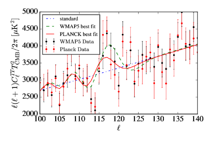
Figure 1: The angular power spectrum of the TT auto-correlation. The black (red) dots and bars show the WMAP5 (Planck2015) data points and their error bars. The green dashed line, the blue dot dashed line and the red solid line represent the best fitting model for the TT and TE combined data of WMAP5 using the oscillating initial power spectrum given by eq.(2), for the TT, TE and EE combined data of Planck2015 using the standard initial power spectrum by eq.(1) and the oscillating initial power spectrum by eq.(2), respectively.

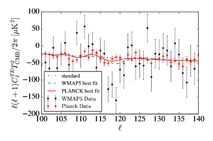
Figure 2: Same as Fig.1 but for the Planck TE cross-correlation data.

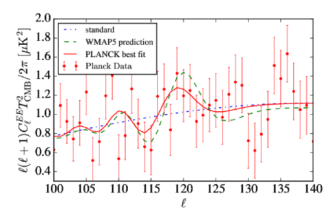
Figure 3: Same as Fig.1 but for the Planck EE auto-correlation data.

The E-mode polarization auto-correlation data have been newly released by the Planck collaboration in 2015. In Fig.3, we can see the prediction by the WMAP5 data fits pretty well to the Planck EE power spectrum. For more accurate understanding of features in the polarization data, we show the likelihoods of the feature parameters in Fig.4. There we show a comparison between the likelihood of the feature parameters only from the TT auto-correlation data and the one from the TT, TE and EE combined data with smaller uncertainties. We can see that all of the likelihoods are sharpened, and the amplitude parameter becomes slightly smaller if we use the combined data. These indicate that there are features with a smaller amplitude, but with the same width and at the same position in the polarization data as in the temperature data.

Table 3 shows the $\chi^{2}$ values are improved by using the oscillating initial power spectrum, and the improvement is more than twice the number of the added parameters. In view of Akaike’s Information Criterion akaike1974 , this implies that the oscillating initial power spectrum (2) is the better model to describe the primordial spectrum of curvature perturbation of our Universe. This does not necessarily mean that inflation model which produced our Universe as it is today must realize such a featured spectrum as a mean value because theoretical cost to realize such an ad hoc spectrum cannot be taken into account in Akaike approach. What is important here is the fact that our Universe is imprinted with such a feature whether it was generated as a result of a non-standard inflation model or as a very rare realization of conventional inflation model predicting a simple power-law spectrum. In either case, in order to determine precise values of cosmological parameters of our Universe, we should incorporate these features in the MCMC analysis.

If they are real imprinted features, they can be seeds of the large scale structure of the universe, and we will be able to see them in the galaxy correlations 2016JCAP…10..041B .

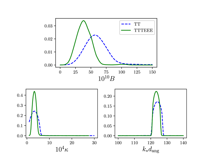
Figure 4: The normalized likelihoods of the amplitude of the oscillations (top), the width (bottom left) and the position (bottom right) from the TT auto-correlation data of Planck2015 (blue dashed line) alone and the TT, TE and EE combined data of Planck2015 (green solid line).

3.2 The effects on the cosmological parameters

We have seen the existence of the features in the Planck data. We need to take into account these features when we estimate the other cosmological parameters. In fact, the inclusion of the features in the initial power spectrum has considerably affected the estimation of cosmological parameters if we use the WMAP5 data 2010PhRvD..81h3010I , especially the estimation of the amplitude of the initial power spectrum $A$ and the spectral index $n_{s}$. From Table 1 and Table 2, we can check the effects of the features on the estimation of the best fit values and the mean values of cosmological parameters for the Planck data. In these tables, the estimated values, including the amplitude $A$ and the spectral index $n_{s}$, have barely changed among the models for each data, namely the standard initial power spectrum, the oscillating initial power spectrum and the fixed oscillation initial power spectrum. From the posterior distributions of some cosmological parameters (Fig.5), we can confirm that the distributions do not vary between the different models of initial power spectrum. These indicate that the local features in the Planck data do not affect the estimation of cosmological parameters. This result is consistent with the analysis for other scales using a similar feature model and Planck data 2014PhRvD..90b3511A ; 2016arXiv161110350T . The improved angular resolution of Planck enables us to observe the greater number of the multipoles at small scales. These rich small scale data has sufficient statistical power to determine the cosmological parameters. This is why the local features do not affect the estimation of the cosmological parameters.

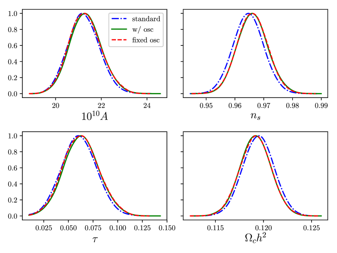
Figure 5: The posterior distributions of the cosmological parameters $10^{9}A$ (top left), $n_{s}$ (top right), $\tau$ (bottom left) and $\Omega_{c}h^{2}$ (bottom right). from the standard power law model (blue solid dot and dash line), oscillations (green solid line), and the fixed oscillation model (red dashed line) derived from the TT, TE and EE combined data.

4 Conclusion

In this paper, we have studied the features at $\ell\sim 120$ in the Planck2015 CMB angular power spectra data which were obtained by the WMAP5 data analysis 2010PhRvD..81h3010I .

We have performed an MCMC analysis using the TT auto-correlation data and TT, TE, EE combined data of the Planck2015, and confirmed the existence of the features in the Planck2015 data. We checked the consistency between the temperature fluctuation data and the polarization data confirming that the features exist in both cases with almost the same width and at the same position albeit a slightly smaller amplitude in the latter data. Then we have investigated effects of these features at $\ell\sim 120$ in determining cosmological parameters and found that they do not affect the estimation of cosmological parameters unlike the case of WMAP5 data, because there are enough data in the higher multipoles to determine the cosmological parameters.

We expect they are the real features of the initial power spectrum and will be observed by the future experiments without interrupting the estimation of the cosmological parameters.

References

- (1) Viatcheslav F. Mukhanov and G. V. Chibisov, JETP Lett., 33, 532–535, [Pisma Zh. Eksp. Teor. Fiz.33,549(1981)] (1981).
- (2) S. W. Hawking, Physics Letters B, 115, 295–297 (September 1982).
- (3) A. H. Guth and S.-Y. Pi, Physical Review Letters, 49, 1110–1113 (October 1982).
- (4) A. A. Starobinsky, Physics Letters B, 117, 175–178 (November 1982).
- (5) A.A. Starobinsky, Physics Letters B, 91(1), 99 – 102 (1980).
- (6) Alan H. Guth, Phys. Rev. D, 23, 347–356 (Jan 1981).
- (7) K. Sato, Mon. Not. R. Astron. Soc., 195, 467–479 (May 1981).
- (8) Katsuhiko Sato and Jun’ichi Yokoyama, Int. J. Mod. Phys., D24(11), 1530025 (2015).
- (9) E. Komatsu, J. Dunkley, M. R. Nolta, C. L. Bennett, B. Gold, G. Hinshaw, N. Jarosik, D. Larson, M. Limon, L. Page, D. N. Spergel, M. Halpern, R. S. Hill, A. Kogut, S. S. Meyer, G. S. Tucker, J. L. Weiland, E. Wollack, and E. L. Wright, apjs, 180, 330–376 (February 2009), 0803.0547.
- (10) Planck Collaboration, P. A. R. Ade, N. Aghanim, M. Arnaud, M. Ashdown, J. Aumont, C. Baccigalupi, A. J. Banday, R. B. Barreiro, J. G. Bartlett, and et al., aap, 594, A13 (September 2016), 1502.01589.
- (11) K. Ichiki, R. Nagata, and J. Yokoyama, Phys. Rev. D, 81(8), 083010 (April 2010), arXiv:0911.5108.
- (12) D. K. Hazra, A. Shafieloo, and G. F. Smoot, JCAP, 12, 035 (December 2013), arXiv:1310.3038.
- (13) A. Ravenni, L. Verde, and A. J. Cuesta, jcap, 8, 028 (August 2016), 1605.06637.
- (14) A. Gallego Cadavid, A. Enea Romano, and S. Gariazzo, ArXiv e-prints (December 2016), 1612.03490.
- (15) Makoto Matsumiya, Misao Sasaki, and Jun’ichi Yokoyama, Phys. Rev., D65, 083007 (2002), arXiv:astro-ph/0111549.
- (16) Makoto Matsumiya, Misao Sasaki, and Jun’ichi Yokoyama, JCAP, 0302, 003 (2003), arXiv:astro-ph/0210365.
- (17) Noriyuki Kogo, Makoto Matsumiya, Misao Sasaki, and Jun’ichi Yokoyama, Astrophys. J., 607, 32–39 (2004), arXiv:astro-ph/0309662.
- (18) Noriyuki Kogo, Misao Sasaki, and Jun’ichi Yokoyama, Prog. Theor. Phys., 114, 555–572 (2005), arXiv:astro-ph/0504471.
- (19) R. Nagata and J. Yokoyama, Phys. Rev. D, 79(4), 043010 (February 2009), 0812.4585.
- (20) D. Tocchini-Valentini, Y. Hoffman, and J. Silk, mnras, 367, 1095–1102 (April 2006), astro-ph/0509478.
- (21) Planck Collaboration, P. A. R. Ade, N. Aghanim, C. Armitage-Caplan, M. Arnaud, M. Ashdown, F. Atrio-Barandela, J. Aumont, C. Baccigalupi, A. J. Banday, and et al., aap, 571, A22 (November 2014), 1303.5082.
- (22) K. Kumazaki, K. Ichiki, N. Sugiyama, and J. Silk, Phys. Rev. D, 87(2), 023008 (January 2013), arXiv:1211.3097.
- (23) P. Hunt and S. Sarkar, JCAP, 1, 025 (January 2014), arXiv:1308.2317.
- (24) D. K. Hazra, A. Shafieloo, and T. Souradeep, JCAP, 11, 011 (November 2014), 1406.4827.
- (25) A. Achúcarro, J.-O. Gong, S. Hardeman, G. A. Palma, and S. P. Patil, JCAP, 1, 030 (January 2011), arXiv:1010.3693.
- (26) S. Céspedes, V. Atal, and G. A. Palma, JCAP, 5, 008 (May 2012), arXiv:1201.4848.
- (27) X. Gao, D. Langlois, and S. Mizuno, JCAP, 10, 040 (October 2012), arXiv:1205.5275.
- (28) R. Saito, M. Nakashima, Y.-i. Takamizu, and J. Yokoyama, JCAP, 11, 036 (November 2012), 1206.2164.
- (29) X. Gao and J.-O. Gong, Journal of High Energy Physics, 8, 115 (August 2015), 1506.08894.
- (30) T. Kobayashi and J. Yokoyama, JCAP, 2, 005 (February 2013), arXiv:1210.4427.
- (31) A. G. Cadavid, A. E. Romano, and S. Gariazzo, European Physical Journal C, 76, 385 (July 2016), 1508.05687.
- (32) M. Nakashima, R. Saito, Y. Takamizu, and J. Yokoyama, Progress of Theoretical Physics, 125, 1035–1052 (May 2011), arXiv:1009.4394.
- (33) A. Achúcarro, V. Atal, B. Hu, P. Ortiz, and J. Torrado, prd, 90(2), 023511 (July 2014), 1404.7522.
- (34) J. Torrado, B. Hu, and A. Achucarro, ArXiv e-prints (November 2016), 1611.10350.
- (35) D. K. Hazra, A. Shafieloo, G. F. Smoot, and A. A. Starobinsky, JCAP, 9, 009 (September 2016), 1605.02106.
- (36) R. Nagata and J. Yokoyama, Phys. Rev. D, 78(12), 123002 (December 2008), 0809.4537.
- (37) K. Kumazaki, S. Yokoyama, and N. Sugiyama, JCAP, 12, 008 (December 2011), 1105.2398.
- (38) A. Lewis and S. Bridle, Phys. Rev. D, 66(10), 103511 (November 2002), astro-ph/0205436.
- (39) Hirotugu Akaike, Automatic Control, IEEE Transactions on, 19(6), 716–723 (December 1974).
- (40) M. Ballardini, F. Finelli, C. Fedeli, and L. Moscardini, jcap, 10, 041 (October 2016), 1606.03747.