Density Estimation for Geolocation via Convolutional Mixture Density Network

Abstract

Nowadays, geographic information related to Twitter is crucially important for fine-grained applications. However, the amount of geographic information avail- able on Twitter is low, which makes the pursuit of many applications challenging. Under such circumstances, estimating the location of a tweet is an important goal of the study. Unlike most previous studies that estimate the pre-defined district as the classification task, this study employs a probability distribution to represent richer information of the tweet, not only the location but also its ambiguity. To realize this modeling, we propose the convolutional mixture density network (CMDN), which uses text data to estimate the mixture model parameters. Experimentally obtained results reveal that CMDN achieved the highest prediction performance among the method for predicting the exact coordinates. It also provides a quantitative representation of the location ambiguity for each tweet that properly works for extracting the reliable location estimations.

(a) I got lost at Umeda station.. Here is almost like a jungle…
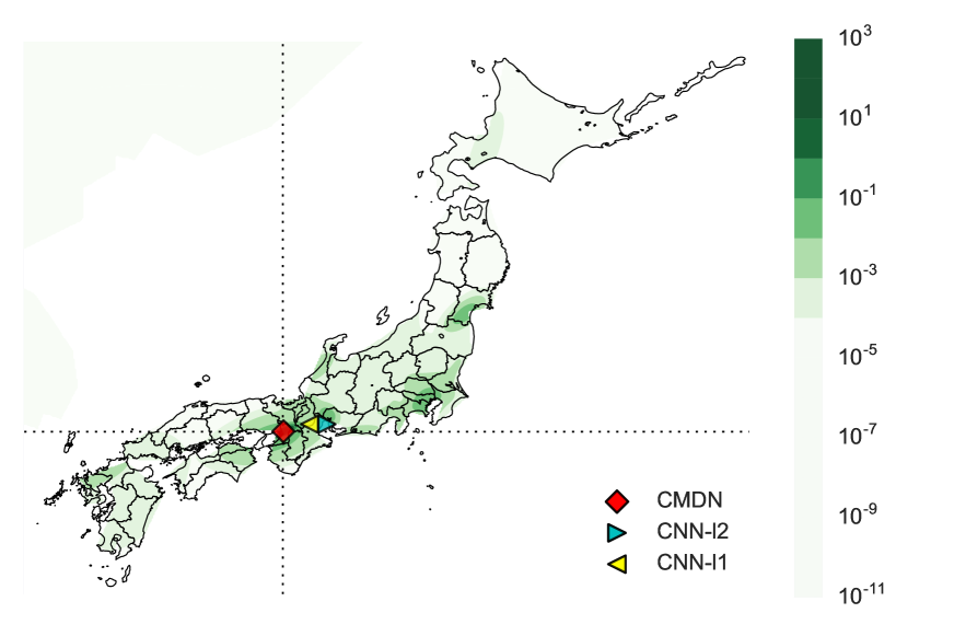
likelihood:195.5, distance: 2.15 (km)

(b) I’ve already slept a lot, but I still feel sleepy…
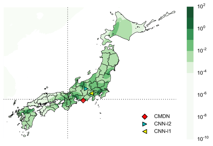
likelihood: 7.0, distance: 174.4 (km)

(c) I will not return to Fukuoka for the first time in Osaka
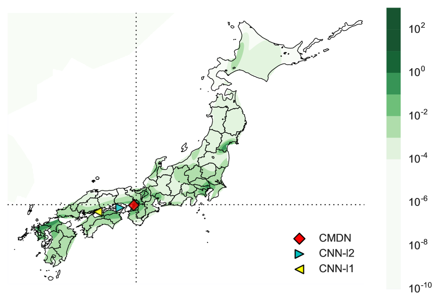
likelihood: 75.6, distance: 13.5 (km)

Figure 1: Original tweet location with the estimated distribution by our proposed method, CMDN. The intersection of dotted line represents the true tweet location. The red diamond represents the estimated location by the CMDN. The blue and yellow triangle represents the CNN for regression with $\ell_{2},\ell_{1}$-loss.

1 Introduction

Geographic information related to Twitter enriches the availability of data resources. Such information is indispensable for various practical applications such as early earthquake detection Sakaki et al. (2010), infectious disease dispersion assessment Broniatowski et al. (2013), and regional user behavior assessment during an election period Caldarelli et al. (2014). However the application performance depends strongly on the number of geo-tagged tweets, which account for fewer than 0.5 % of all tweets Cheng et al. (2010).

To extend the possibilities of the geographic information, a great deal of effort has been devoted to specifying the geolocation automatically Han et al. (2014). These studies are classified roughly into two aspects, the User level Cheng et al. (2010); Han et al. (2014); Jurgens et al. (2015); Rahimi et al. (2015) and the Message level Dredze et al. (2016); Liu and Huang (2016); Priedhorsky et al. (2014) prediction. The former predicts the residential area. The latter one predicts the place that the user mentioned. This study targeted the latter problem, with message level prediction, involving the following three levels of difficulty.

First, most tweets lack information to identify the true geolocation. In general, many tweets do not include geolocation identifiable words. Therefore, it is difficult even for humans to identify a geolocation (Figure 1(b)).

Next, some location names involve ambiguity because a word refers to multiple locations. For example, places called “Portland” exist in several locations worldwide. Similarly, this ambiguity also arises within a single country, as shown in Figure 2. Although additional context words are necessary to identify the exact location, many tweets do not include such clue words for identifying the location. As for such tweet, the real-valued point estimation is expected to be degraded by regression towards the mean Stigler (1997).

Finally, if a user states the word that represents the exact location, the user is not necessarily there. In case the user describes several places in the tweet, contextual comprehension of the tweet is needed to identify the true location (Figure 1(c)).

In contrast to most studies, this study was conducted to resolve these issues based on the density estimation approach. A salient benefit of density estimation is to enable comprehension of the uncertainty related to the tweet user location because it propagates from the estimated distribution and handles tweets distributed to multiple points properly. Figure 1 shows each estimated density as a heatmap. The estimated distribution is concentrated near the true location (Figure 1(a)) and vice versa (Figure 1(b)) if the tweet includes plenty of clues. Furthermore, the density-based approach can accommodate the representation of multiple output data, whereas the regression-based approach cannot (Figure 1(c)).

The density-based approach provides additional benefits for practical application. The estimated density appends the estimation reliability for each tweet as the likelihood value. For reliable estimation, the estimated density provides the high likelihood (Figure 1(a) and 1(c)) and vice versa (Figure 1(b)).

To realize this modeling, we propose a Convolutional Mixture Density Network (CMDN), a method for estimating the geolocation density estimation from text data. Actually, CMDN extracts valuable features using a convolutional neural network architecture and converts these features to mixture density parameters. Our experimentally obtained results reveal that not merely the high prediction performance, but also the reliability measure works properly for filtering out uncertain estimations.

2 Related work

Social media geolocation has been undertaken on various platforms such as Facebook Backstrom et al. (2010), Flickr Serdyukov et al. (2009), and Wikipedia Lieberman and Lin (2009). Especially, Twitter geolocation is the predominant field among all of them because of its availability Han et al. (2014).

Twitter geolocation methods are not confined to text information. Diverse information can facilitate geolocation performance such as meta information (time Dredze et al. (2016) and estimated age and gender Pavalanathan and Eisenstein (2015)), social network structures Jurgens et al. (2015); Rahimi et al. (2015), and user movement Liu and Huang (2016). Many studies, however, have attempted user level geolocation, not the message level. Although the user level geolocation is certainly effective for some applications, message level geolocation supports fine-grained analyses.

However, Priedhorsky et al. (2014) has attempted density estimation for message level geolocation by estimating a word-independent Gaussian Mixture Model and then combining them to derive each tweet density. Although the paper proposed many weight estimation methods, many of them depend strongly on locally distributed words. Our proposed method, CMDN, enables estimate of the geolocation density from the text sequence in the End-to-End manner and considers the marginal context of the tweet via CNN.

Figure 2: The places where the word “Sakurajima” was mentioned in training data are projected on the map. The word “Sakurajima” is mentioned in multiple places because this word represents multiple locations.

3 Convolutional Neural Network for Regression (Unimodal output)

We start by introducing the convolutional neural network Fukushima (1980); LeCun et al. (1998) (CNN) for a regression problem, which directly estimates the real-valued output as our baseline method. Our regression formulation is almost identical to that of CNN for document classification based on Kim (2014). We merely remove the softmax layer and replace the loss function.

We assume that a tweet has length $L$ (padded where necessary) and that $w_{i}$ represents the word $i$-th index. We project the words $\mathbf{w}_{i}$ to vectors $\mathbf{x}_{i}$ through an embedding matrix $\mathbf{W}_{e}$, $\mathbf{x}_{i}=\mathbf{W}_{e}\mathbf{w}_{i}\in\mathbb{R}^{d}$, where $d$ represents the size of the embeddings. We compose the sentence vector $\mathbf{x}_{1:L}$ by concatenating the word vectors $\mathbf{x}_{i}$, as

$$\mathbf{x}_{1:L}=\mathbf{x}_{1}\oplus\mathbf{x}_{2}\oplus\dots\oplus\mathbf{x}_{L}\in\mathbb{R}^{Ld}.$$

In that equation, $\oplus$ represents vector concatenation.

To extract valuable features from sentences, we apply filter matrix $\mathbf{W}_{f}$ for every part of the sentence vector with window size $\ell$ as

$$\mathbf{W}_{f} =[\mathbf{w}_{f,1},\mathbf{w}_{f,2},\dots,\mathbf{w}_{f,m}]^{\top}$$

$$c_{i,j} =\phi(\mathbf{w}_{f,j}^{\top}\mathbf{x}_{i:i+\ell}+b_{f,j})$$

where $m$ stands for the number of feature maps, and $\phi$ represents the activation function. As described herein, we employ ReLU Nair and Hinton (2010) as the activation function.

For each filter’s output, we apply 1-max pooling to extract the most probable window feature $\hat{c}_{j}$. Then we compose the abstracted feature vectors $\mathbf{h}$ by concatenating each pooled feature $\hat{c}_{j}$ as shown below.

$$\hat{c}_{j} =\max_{i\in\left\{1,\dots,L-\ell+1\right\}}c_{i,j}$$

$$\mathbf{h} =[\hat{c}_{1},\hat{c}_{2},\dots,\hat{c}_{m}]^{\top}$$

Finally, we estimate the real value output $\mathbf{y}$ using the abstracted feature vector $\mathbf{h}$ as

$$\hat{\mathbf{y}}=\mathbf{W}_{r}\mathbf{h}+\mathbf{b}_{r}\in\mathbb{R}^{q}$$

where $q$ signifies the output dimension, $\mathbf{W}_{r}\in\mathbb{R}^{q\times m}$, denotes the regression weight matrix, and $\mathbf{b}_{r}\in\mathbb{R}^{q}$ represent the bias vectors for regression.

To optimize the regression model, we use two loss functions between the true value $\mathbf{y}$ and estimated value $\hat{\mathbf{y}}$. One is $\ell_{2}$-loss as

$$\sum_{n=1}^{N}\|\mathbf{y}_{n}-\hat{\mathbf{y}}_{n}\|^{2}_{2}$$

and another is robust loss function for outlier, $\ell_{1}$-loss,

$$\sum_{n=1}^{N}\|\mathbf{y}_{n}-\hat{\mathbf{y}}_{n}\|_{1}=\sum_{n=1}^{N}\sum_{q^{\prime}=1}^{q}|{y}_{n,q^{\prime}}-\hat{y}_{n,q^{\prime}}|$$

where $N$ represents the sample size. The $\ell_{1}$-loss shrinks the outlier effects for estimation rather than the $\ell_{2}$ one.

4 Convolutional Mixture Density Network (Multimodal output)

In the previous section, we introduced the CNN method for regression problem. This regression formulation is good for addressing well-defined problems. Both the input and output have one-to-one correspondence. Our tweet corpus is fundamentally unfulfilled with this assumption. Therefore, a more flexible model must be used to represent the richer information.

In this section, we propose a novel architecture for text to density estimation, Convolutional Mixture Density Network (CMDN), which is the extension of Mixture Density Network by Bishop (1994). In contrast to the regression approach that directly represents the output values $\hat{\mathbf{y}}$, CMDN can accommodate more complex information as the probability distribution. The CMDN estimates the parameters of Gaussian mixture model $\pi_{k},\bm{\mu}_{k},\bm{\Sigma}_{k}$, where $k$ is the $k$-th mixture component using the same abstracted features $\mathbf{h}$ in the CNN regression (Sec 3).

4.1 Parameter estimation by neural network

Presuming that density consists of $K$ components of multivariate normal distribution $\mathcal{N}(\mathbf{y}|\bm{\mu}_{k},\bm{\Sigma}_{k})$, then the number of each $q$-dimensional normal distribution parameters are $p=\frac{q(q+3)}{2}$ ($q$ parameters for each mean $\bm{\mu}_{k}$ and diagonal values of the covariance matrix $\bm{\Sigma}_{k}$ and $\frac{q(q-1)}{2}$ parameters for correlation parameters $\rho$) between dimension outputs.

For $q=2$, each component of the parameters is represented as

$$\bm{\mu}_{k}=\begin{pmatrix}\mu_{k,1}\\ \mu_{k,2}\end{pmatrix},\bm{\Sigma}_{k}=\begin{pmatrix}\sigma_{k,1}^{2}&\rho_{k}\sigma_{k,1}\sigma_{k,2}\\ \rho_{k}\sigma_{k,1}\sigma_{k,2}&\sigma_{k,2}^{2}\end{pmatrix}.$$

To estimate these parameters, we first project the hidden layer $\mathbf{h}$ into the required number of parameters space $\bm{\theta}$ as

$$\bm{\theta}=\mathbf{W}_{p}\mathbf{h}+\mathbf{b}_{p}\in\mathbb{R}^{Kp},$$

where $\mathbf{W}_{p}\in\mathbb{R}^{Kp\times m}$ and $\mathbf{b}_{p}\in\mathbb{R}^{Kp}$ respectively denote the weight matrix and bias vector.

Although the parameter $\bm{\theta}$ has a sufficient number of parameters to represent the $K$ mixture model, these parameters are not optimal for insertion to the parameters of the multivariate normal distribution $\mathcal{N}(\mathbf{y}|\bm{\mu}_{k},\bm{\Sigma}_{k})$, and its mixture weight $\pi_{k}$.

The mixture weights $\pi_{k}$ must be positive values and must sum to 1. The variance parameters $\sigma$ must be a positive real value. The correlation parameter $\rho_{k}$ must be $(-1,1)$. For this purpose, we transform real-valued outputs $\bm{\theta}$ into the optimal range for each parameter of mixture density.

4.2 Parameter conversion

For simplicity, we first decompose $\bm{\theta}$ to each mixture parameter $\bm{\theta}_{k}$ as

$$\bm{\theta} =\bm{\theta}_{1}\oplus\bm{\theta}_{2}\oplus\dots\oplus\bm{\theta}_{K}$$

$$\bm{\theta}_{k} =(\theta_{\pi_{k}},\theta_{\mu_{k,1}},\theta_{\mu_{k,2}},\theta_{\sigma_{k,1}},\theta_{\sigma_{k,2}},\theta_{\rho_{k}}).$$

To restrict each parameter range, we convert each vanilla parameter $\bm{\theta}_{k}$ as

$$\pi_{k} =\mbox{softmax}(\theta_{\pi_{k}})$$

$$=\frac{\exp(\theta_{\pi_{k}})}{\sum_{k^{\prime}=1}^{K}\exp(\theta_{\pi_{k}^{\prime}})}\in(0,1)$$

$$\mu_{k,j} =\theta_{\mu_{k,j}}\in\mathbb{R},$$

$$\sigma_{k,j} =\mbox{softplus}(\theta_{\sigma_{k,j}})$$

$$=\ln\left(1+\exp(\theta_{\sigma_{k,j}})\right)\in(0,\infty),$$

$$\rho_{k} =\mbox{softsign}(\theta_{\rho_{k}})$$

$$=\frac{\theta_{\rho_{k}}}{1+|\theta_{\rho_{k}}|}\in(-1,1).$$

The original MDN paper Bishop (1994) and its well known application of MDN for handwriting generation Graves (2013) used an exponential function for transforming variance parameter $\sigma$ and a hyperbolic tangent function for the correlation parameter $\rho$. However, we use softplus Glorot et al. (2011) for variance and softsign Glorot and Bengio (2010) for correlation.

Replacing the activation function in the output layer prevents these gradient problems. Actually, these gradient values are often exploded or nonexistent. Our proposed transformation is effective to achieve rapid convergence and stable learning.

4.3 Loss function for parameter estimation

To optimize the mixture density model, we use negative log likelihood as the training loss:

$$-\sum_{n=1}^{N}\ln\left(\sum_{k=1}^{K}\pi_{k}\mathcal{N}(\mathbf{y}_{n}|\bm{\mu}_{k},\bm{\Sigma}_{k})\right).$$

5 Experiments

In this section, we formalize our problem setting and clarify our proposed model effectiveness.

5.1 Problem setting

This study explores CMDN performance from two perspectives.

Our first experiment is to predict the geographic coordinates by which each user stated using the only single tweet content. We evaluate the mean and median value of distances measured using Vincenty’s formula Vincenty (1975) between the estimated and true geographic coordinates for the overall dataset.

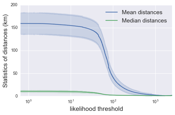
The second experiment is used to filter out the unreliable estimation quantitatively using the likelihood-based threshold. Each estimated density assigns the likelihood value for every point of the location. We designate the likelihood values as reliability indicators for the respective estimated locations. Then, we remove the estimation from the lowest likelihood value and calculate both the mean and median values. This indicator is filtered correctly out the unreliable estimations if the statistics decrease monotonically.

Location estimation by estimated density

In contrast to the regression approach, it is necessary to specify the estimation point from the estimated density of each tweet. In accordance with Bishop (1994), we employ the mode value of estimated density as the estimated location $\hat{\mathbf{y}}$. The mode value of the probability distribution can be found by numerical optimization, but it requires overly high costs for scalable estimation. For a simple and scalable approximation for seeking the mode value of the estimated density, we restrict the search space to each mean value of the mixture components as shown below:

$$\hat{\mathbf{y}}=\operatorname*{argmax}_{\mathbf{y}\in\{\bm{\mu}_{1},\dots,\bm{\mu}_{K}\}}\sum_{k=1}^{K}\pi_{k}\mathcal{N}(\mathbf{y}|\bm{\mu}_{k},\bm{\Sigma}_{k}).$$

5.2 Dataset

Our tweet corpus consists of 24,633,478 Japanese tweets posted from July 14, 2011 to July 31, 2012. Our corpus statistics are presented in Table 1. We split our corpus randomly into training for 20M tweets, development for 2M, and test for 2M.

Dataset
# of tweets	24,633,478
# of users	276,248
Average # of word	16.0
# of vocabulary	351,752

Table 1: Dataset statistics.

5.3 Comparative models

We compare our proposed model effectiveness by controlling experiment procedures, which replace the model components one-by-one. We also provide simple baseline performance. The following model configurations are presented in Table 2.

Mean: Mean value of the training data locations.

Median: Median value of the training data locations.

Enet: Elastic Net regression Zou and Hastie (2005), which consists of ordinary least squares regression with $\ell_{2},\ell_{1}$-regularization.

MLP-l2: Multi Layer Perceptron with $\ell_{2}$-loss Minsky and Papert (1969)

MLP-l1: Multi Layer Perceptron with $\ell_{1}$-loss.

CNN-l2: Convolutional Neural Network for regression with $\ell_{2}$-loss based on Kim (2014)

CNN-l1: Convolutional Neural Network for regression with $\ell_{1}$-loss.

MDN: Mode value of Mixture Density Network Bishop (1994)

CMDN: Mode value of Convolutional Mixture Density Network (Proposed)

Parameters
# of mixture	50
Embedding dimension	300
Window sizes	3, 4, 5
Each filter size	128
Dropout rate Srivastava et al. (2014)	0.2
Batch size	500
Learning rate	0.0001
Optimization	Adam Kingma and Ba (2014)

Table 2: Model configurations.

5.4 Results

5.4.1 Geolocation performance

The experimental geolocation performance results are presented in Table 3.

Overall results show that our proposed model CMDN provides the lowest median error distance: CNN-l1 is the lowest mean error distance. Also, CMDN gives similar mean error distances to those of CNN-l1. Both CMDN and CNN-l1 outperform all others in comparative models.

In addition to the results obtained for the feature extraction part, the CNN-based model consistently achieved better prediction performance than the vanilla MLP-based model measured by both the mean and median.

Method	Mean (km)	Median (km)
CMDN	159.4	10.7
CNN-l1	147.5	28.2
CNN-l2	166.5	80.5
MDN	251.4	92.9
MLP-l1	224.0	75.0
MLP-l2	226.8	140.3
Enet	197.2	144.6
Mean	279.4	173.9
Median	253.7	96.1

Table 3: The prediction performance. The lower value is the better estimation.

5.4.2 Likelihood based threshold

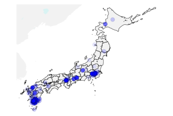
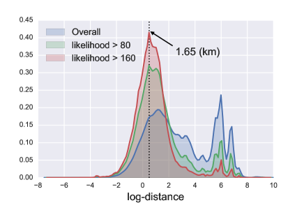
We show how the likelihood-based threshold affects both mean and median statistics in Figure 3. The likelihood-based threshold consistently decreases both statistics in proportion to the likelihood lower bound increases. Especially, these statistics dramatically decrease when the likelihood is between $10^{1}$ and $10^{2}$. Several likelihood bounds results are presented in Figure 4. Although the model mistakenly estimates many incorrect predictions for the overall dataset (blue), the likelihood base threshold correctly prunes the outlier estimations.

Figure 3: Likelihood-based threshold results with 95% confidence interval for our proposed model: CMDN. To extract reliable (lower value of distance measures) geolocated tweets, we can increase the lower bound of likelihood. The standard deviations of both the mean and median are calculated using Bootstrap methods Efron (1979).

Figure 4: Output distribution with several likelihood thresholds. The small log-distance represents the better prediction.

6 Discussion

Our proposed model provides high accuracy for our experimental data. Moreover, likelihood-based thresholds reveal a consistent indicator of estimation certainty. In this section, we further explore the properties of the CMDN from the viewpoint of difference of the loss function.

Loss function difference

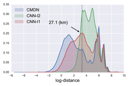
We compare the CNN-based model with different loss functions, $\ell_{2},\ell_{1}$-loss for regression CNN-l2, CNN-l1 and negative log-likelihood for mixture density model CMDN. The output distance distributions are shown in Figure 5.

Although $\ell_{2}$-loss denotes the worst performance measured by mean and median among CNN-based models (Table 3), it represents the lowest outlier ratio. Consequently, the $\ell_{2}$-loss is the most conservative estimate for our skewed corpus.

We can infer that the difference between the competitive model CNN-l1 and our proposed model CMDN is their estimation aggressiveness. The median of CMDN is remarkably lower than of CNN-l1, but the mean of CMDN is slightly larger than that of CNN-l1. The reason for these phenomena is the difference of the loss functions behavior for multiple candidate data. Even though the $\ell_{1}$-loss function is robust to outliers, the estimation deteriorates when the candidates appear with similar possibilities. In contrast, CMDN can accommodate multiple candidates as multiple mixture components. Therefore, CMDN imposes the appropriate probabilities for several candidates and picks up the most probable point as the prediction. In short, CMDN’s predictions become more aggressive than CNN-l1’s. Consequently, CMDN’s median value becomes lower than CNN-l1’s.

An important shortcoming of aggressive prediction is that the estimation deteriorates when the estimation fails. The mean value tends to be affected strongly by the outlier estimation. Therefore, CMDN’s mean value becomes higher than that of CNN-l1’s.

However, CMDN can overcome this shortcoming using a likelihood-based threshold, which first filters out the outlier. Therefore, we conclude that the negative log-likelihood for mixture density is better than those of other loss functions $\ell_{2}$ and $\ell_{1}$-loss for the regression.

Figure 5: Loss function difference: Lower values represent better predictions. Our proposed model, CMDN (blue), tends to be the most aggressive estimation.

7 Future work

This study assessed the performance of our proposed model, CMDN, using text data alone. Although text-only estimation is readily applicable to existing resources, we still have room for improvement of the prediction performance. The winner of the Twitter Geolocation Prediction Shared Task, Miura et al. (2016), proposed that the unified architecture handle several meta-data such as the user location, user description, and time zone for predicting geolocations. The CMDN can integrate this information in the same manner.

Furthermore, Liu and Huang (2016) reports that the user home location strongly affects location prediction for a single tweet. For example, a routine tweet is fundamentally unpredictable using text contents alone, but if the user home location is known, this information is a valuable indication for evaluating the tweet. As future work, we plan to develop a unified architecture that incorporates user movement information using a recurrent neural network.

In contrast, our objective function might be no longer useful for world scale geolocation because ours approximates the spherical coordinates into the real coordinate space. This approximation error tends to become larger for the larger scale geolocation inference. We will explore our method’s geolocation performance using the world scale geolocation dataset such as W-NUT data Han et al. (2016).

8 Conclusion

This study clarified the capabilities of the density estimation approach to Twitter geolocation. Our proposed model, CMDN, performed not only with high accuracy for our experimental data; it also extracted reliable geolocated tweets using likelihood-based thresholds. Results show that CMDN merely requires the tweet message contents to identify its geolocation, while obviating preparation of meta-information. Consequently, CMDN can contribute to extension of the fields in which geographic information application can be used.

References

- Backstrom et al. (2010) Lars Backstrom, Eric Sun, and Cameron Marlow. 2010. Find me if you can: improving geographical prediction with social and spatial proximity. In Proceedings of the 19th international conference on World wide web. ACM, pages 61–70.
- Bishop (1994) Christopher Bishop. 1994. Mixture density networks. Technical report.
- Broniatowski et al. (2013) David A. Broniatowski, Michael J. Paul, and Mark Dredze. 2013. National and local influenza surveillance through twitter: An analysis of the 2012-2013 influenza epidemic. PLoS ONE 8(12). https://doi.org/10.1371/journal.pone.0083672.
- Caldarelli et al. (2014) Guido Caldarelli, Alessandro Chessa, Fabio Pammolli, Gabriele Pompa, Michelangelo Puliga, Massimo Riccaboni, and Gianni Riotta. 2014. A multi-level geographical study of italian political elections from twitter data. PLoS ONE 9(5):1–11. https://doi.org/10.1371/journal.pone.0095809.
- Cheng et al. (2010) Zhiyuan Cheng, James Caverlee, and Kyumin Lee. 2010. You are where you tweet: A content-based approach to geo-locating twitter users. In Proceedings of the 19th ACM International Conference on Information and Knowledge Management. ACM, New York, NY, USA, CIKM ’10, pages 759–768. https://doi.org/10.1145/1871437.1871535.
- Dredze et al. (2016) Mark Dredze, Miles Osborne, and Prabhanjan Kambadur. 2016. Geolocation for twitter: Timing matters. In North American Chapter of the Association for Computational Linguistics (NAACL).
- Efron (1979) B Efron. 1979. Bootstrap methods: Another look at the jackknife. The Annals of Statistics pages 1–26.
- Fukushima (1980) Kunihiko Fukushima. 1980. Neocognitron: A self-organizing neural network model for a mechanism of pattern recognition unaffected by shift in position. Biological cybernetics 36(4):193–202.
- Glorot and Bengio (2010) Xavier Glorot and Yoshua Bengio. 2010. Understanding the difficulty of training deep feedforward neural networks. In Aistats. volume 9, pages 249–256.
- Glorot et al. (2011) Xavier Glorot, Antoine Bordes, and Yoshua Bengio. 2011. Deep sparse rectifier neural networks. In Aistats. volume 15, page 275.
- Graves (2013) Alex Graves. 2013. Generating sequences with recurrent neural networks. arXiv preprint arXiv:1308.0850 .
- Han et al. (2014) Bo Han, Paul Cook, and Timothy Baldwin. 2014. Text-based twitter user geolocation prediction. Journal of Artificial Intelligence Research 49:451–500. https://doi.org/10.1613/jair.4200.
- Han et al. (2016) Bo Han, AI Hugo, Afshin Rahimi, Leon Derczynski, and Timothy Baldwin. 2016. Twitter geolocation prediction shared task of the 2016 workshop on noisy user-generated text. WNUT 2016 page 213.
- Jurgens et al. (2015) David Jurgens, Tyler Finethy, James McCorriston, Yi Tian Xu, and Derek Ruths. 2015. Geolocation prediction in twitter using social networks: A critical analysis and review of current practice. In ICWSM. pages 188–197.
- Kim (2014) Yoon Kim. 2014. Convolutional neural networks for sentence classification. In Proceedings of the 2014 Conference on Empirical Methods in Natural Language Processing (EMNLP). Association for Computational Linguistics, Doha, Qatar, pages 1746–1751. http://www.aclweb.org/anthology/D14-1181.
- Kingma and Ba (2014) Diederik Kingma and Jimmy Ba. 2014. Adam: A method for stochastic optimization. arXiv preprint arXiv:1412.6980 .
- LeCun et al. (1998) Yann LeCun, Léon Bottou, Yoshua Bengio, and Patrick Haffner. 1998. Gradient-based learning applied to document recognition. Proceedings of the IEEE 86(11):2278–2324.
- Lieberman and Lin (2009) Michael D Lieberman and Jimmy J Lin. 2009. You are where you edit: Locating wikipedia contributors through edit histories. In ICWSM.
- Liu and Huang (2016) Zhi Liu and Yan Huang. 2016. Where are you tweeting?: A context and user movement based approach. In Proceedings of the 25th ACM International on Conference on Information and Knowledge Management. ACM, New York, NY, USA, CIKM ’16, pages 1949–1952. https://doi.org/10.1145/2983323.2983881.
- Minsky and Papert (1969) Marvin Minsky and Seymour Papert. 1969. Perceptrons: An Introduction to Computational Geometry. MIT Press, Cambridge, MA, USA.
- Miura et al. (2016) Yasuhide Miura, Motoki Taniguchi, Tomoki Taniguchi, and Tomoko Ohkuma. 2016. A simple scalable neural networks based model for geolocation prediction in twitter. WNUT 2016 9026924:235.
- Nair and Hinton (2010) Vinod Nair and Geoffrey E Hinton. 2010. Rectified linear units improve restricted boltzmann machines. In Proceedings of the 27th international conference on machine learning (ICML-10). pages 807–814.
- Pavalanathan and Eisenstein (2015) Umashanthi Pavalanathan and Jacob Eisenstein. 2015. Confounds and consequences in geotagged twitter data. In Proceedings of Empirical Methods for Natural Language Processing (EMNLP). http://www.aclweb.org/anthology/D/D15/D15-1256.pdf.
- Priedhorsky et al. (2014) Reid Priedhorsky, Aron Culotta, and Sara Y Del Valle. 2014. Inferring the origin locations of tweets with quantitative confidence. In Proceedings of the 17th ACM conference on Computer supported cooperative work & social computing. ACM, pages 1523–1536.
- Rahimi et al. (2015) Afshin Rahimi, Duy Vu, Trevor Cohn, and Timothy Baldwin. 2015. Exploiting text and network context for geolocation of social media users. In Proceedings of the 2015 Conference of the North American Chapter of the Association for Computational Linguistics: Human Language Technologies. Association for Computational Linguistics, Denver, Colorado, pages 1362–1367. http://www.aclweb.org/anthology/N15-1153.
- Sakaki et al. (2010) Takeshi Sakaki, Makoto Okazaki, and Yutaka Matsuo. 2010. Earthquake shakes twitter users: Real-time event detection by social sensors. In Proceedings of the 19th International Conference on World Wide Web. ACM, New York, NY, USA, WWW ’10, pages 851–860. https://doi.org/10.1145/1772690.1772777.
- Serdyukov et al. (2009) Pavel Serdyukov, Vanessa Murdock, and Roelof Van Zwol. 2009. Placing flickr photos on a map. In Proceedings of the 32nd international ACM SIGIR conference on Research and development in information retrieval. ACM, pages 484–491.
- Srivastava et al. (2014) Nitish Srivastava, Geoffrey E Hinton, Alex Krizhevsky, Ilya Sutskever, and Ruslan Salakhutdinov. 2014. Dropout: a simple way to prevent neural networks from overfitting. Journal of Machine Learning Research 15(1):1929–1958.
- Stigler (1997) Stephen M Stigler. 1997. Regression towards the mean, historically considered. Statistical methods in medical research 6(2):103–114.
- Vincenty (1975) Thaddeus Vincenty. 1975. Direct and inverse solutions of geodesics on the ellipsoid with application of nested equations. Survey review 23(176):88–93.
- Zou and Hastie (2005) Hui Zou and Trevor Hastie. 2005. Regularization and variable selection via the elastic net. Journal of the Royal Statistical Society: Series B (Statistical Methodology) 67(2):301–320.