Abstract

We discuss the implications of studies of partition function zeros and equimodular curves for the analytic properties of the Ising model on a square lattice in a magnetic field. In particular we consider the dense set of singularities in the susceptibility of the Ising model at $H=0$ found by Nickel and its relation to the analyticity of the field theory computations of Fonseca and Zamolodchikov.

Analyticity of the Ising susceptibility:
An interpretation

1 Introduction

The magnetic susceptibility at $H=0$ of the two dimensional Ising model on a square lattice was shown in 1999 by Nickel [1, 2] to have the remarkable (and unexpected) property that as a function of a complex temperature variable there is a dense set of singularities at the locus of the zeros of the $H=0$ partition function of the finite size lattice.

On the other hand in 2003 Fonseca and Zamolodchikov [4] presented a compelling scenario, since supported by extensive numerical studies [5, 6], for the behavior of the Ising model in a magnetic field in the scaling field theory limit which assumes analyticity at the locus of singularities.

The compatibility of these two approaches is an open question which needs to be understood.

In this paper we investigate this compatibility by means of studying the dependence on the magnetic field of the temperature zeros of the finite size partition function and of the equimodular curves of the corresponding transfer matrix. This will use and extend the work of [7]. It would be highly desirable to treat these questions of analyticity by rigorous mathematical methods but, somewhat surprisingly, we will see that the needed tools do not seem to exist.

In section 2 we give a precise formulation of the problem. The partition function zeros are studied in section 3 and the transfer matrix eigenvalues in section 4. In section 5 we use these studies to formulate an interpretation which reconciles the singularities of Nickel with the analyticity of Fonseca and Zamolodchikov. Our conclusions are summarized in section 6.

2 Formulation

The isotropic two dimensional Ising model on a square lattice in the presence of a magnetic field is defined by the interaction energy

$${\mathcal{E}}=-\sum_{j,k}(E\sigma_{j,k}\sigma_{j+1,k}+E\sigma_{j,k}\sigma_{j,k+1}+H\sigma_{j,k})$$ (1)

where $\sigma_{j,k}=\pm 1$ is the spin at row $j$ and column $k$ and the sum is over all spins in a lattice of $L_{v}$ rows and $L_{h}$ columns with either cylindrical or toroidal boundary conditions or the boundary conditions of Brascamp-Kunz [8] where on a finite cylinder (with periodic boundary conditions in the $L_{h}$ direction) one end interacts with a fixed row of up spins and the other end interacts with an alternating row of up and down spins with $L_{h}$ is even.

The partition function on the $L_{v}\times L_{h}$ lattice at temperature $T$ is defined as

$$Z_{L_{v},L_{h}}=\sum_{\sigma=\pm 1}e^{-\beta{\mathcal{E}}}$$ (2)

where $\beta=1/k_{B}T$ (with $k_{B}$ being Boltzmann’s constant). $Z_{L_{v},L_{h}}$ is a polynomial in the variables $u=e^{-2E/k_{B}T}~{}~{}{\rm and}~{}~{}x=e^{-2H/k_{B}T}$. However, we note that for appropriate boundary conditions including Brascamp-Kunz [8] and toriodal (but not cylindrical) the dependence is only on $u^{2}$. The thermodynamic limit is the limit where $L_{v},L_{h}\rightarrow\infty$ with $L_{v}/L_{h}$ fixed away from zero and infinity. The free energy is defined in the thermodynamic limit as

$$-F/k_{B}T=\lim_{L_{v},L_{h}\rightarrow\infty}\frac{1}{L_{v}L_{h}}\ln Z_{L_{v},L_{h}}.$$ (3)

At $H=0$ the free energy of the Ising model is [9]

$$-F/k_{B}T=\frac{1}{2}\ln(2s)+\frac{1}{8\pi^{2}}\int_{-\pi}^{\pi}d\theta_{1}\int_{-\pi}^{\pi}d\theta_{2}\ln(s+s^{-1}-\cos\theta_{1}-\cos\theta_{2})$$ (4)

where

$$s=\sinh(2E/k_{B}T)=\frac{u^{-1}-u}{2}.$$ (5)

This integral has a singularity at a temperature $T_{c}$ such that $s_{c}=\pm 1$, where negative $s$ implies that $E$ is negative and hence that the system is antiferromagnetic.

For $H=0$ the zeros of the partition function accumulate in the thermodynamic limit on the circle

$$|s|=1$$ (6)

which in terms of the variable $u$ becomes the two circles

$$u=\pm 1+2^{1/2}e^{i\theta}~{}~{}~{}{\rm with}~{}0\leq\theta<2\pi$$ (7)

and the ferromagnetic (antiferromagnetic) critical temperatures are given by

$$u_{c}=\sqrt{2}-1~{}~{}{\rm ferromagnetic},~{}~{}~{}u_{c}=\sqrt{2}+1~{}~{}{\rm antiferromagnetic}.$$ (8)

For Brascamp-Kunz boundary conditions all the zeros of the partition function for $H=0$ are exactly on the unit circle at the positions

$$s+s^{-1}=\cos\frac{(2n-1)\pi}{L_{h}}+\cos\frac{m\pi}{L_{v}+1}$$ (9)

with $1\leq n\leq L_{h}/2,~{}1\leq m\leq L_{v},$ and $L_{h}$ even.

The magnetic susceptibility is given as the second derivative of the free energy with respect to $H$ as

$$\chi=\frac{\partial M(H)}{\partial H}=k_{B}T\frac{\partial^{2}\ln Z}{\partial H^{2}}.$$ (10)

In 1999/2000 Nickel [1, 2] discovered that in the thermodynamic limit for both $T<T_{c}$ and $T>T_{c}$ the susceptibility has an infinite number of singularities on the circle $|s|=1$ at

$$s_{j}+s_{j}^{-1}=\cos(2\pi m/j)+\cos(2\pi n/j)$$ (11)

where

$$0\leq m,n\leq j-1~{}{\rm with}~{}m=n=0~{}{\rm excluded}.$$ (12)

Here $j$ is a positive integer which is odd for $T>T_{c}$ and the singularity at $s_{j}$ is proportional to

$$\epsilon^{2j(j-1)-1}\ln\epsilon$$ (13)

where $\epsilon=s-s_{j}$. For $T<T_{c}$ the integer $j$ is even and the singularity at $s_{j}$ is proportional to

$$\epsilon^{2j^{2}-3/2}.$$ (14)

3 Partition function zeros

The partition function depends on the two variables $x$ and $u$ and in principle should be considered as a polynomial in two variables. However, here we will consider the dependence on $x$ and $u$ separately and not jointly.

3.1 Dependence on $x$

The earliest study of partition function zeros is for zeros in the plane of $x=e^{-2H/k_{B}T}$ for fixed values of $u=e^{-2E/k_{B}T}$ where for ferromagnetic interactions $E>0$ and for free, toroidal or cylindrical boundary conditions Lee and Yang [10] proved that the zeros all lie on the unit circle $|x|=1$

$$Z_{L_{v},L_{h}}(x)=x^{-N/2}\prod_{n=1}^{N}(x-e^{i\theta_{n}^{(N)}})$$ (15)

where $N=L_{v}L_{h}$ and $\theta_{n}^{(N)}$ is real and satisfies

$$\theta^{(N)}_{n}=-\theta^{(N)}_{N-n}$$ (16)

and we note that $Z_{L_{v},L_{h}}(x)=Z_{L_{v},L_{h}}(x^{-1})$. For $T<T_{c}$, where $0\leq u<{\sqrt{2}}-1,$ the zeros lie on the entire circle $|x|=1$ and for $T>T_{c}$, where ${\sqrt{2}}-1<u\leq 1,$ the zeros lie on an arc $x=e^{i\theta}$ where $0<\theta_{LY}\leq\theta\leq 2\pi-\theta_{LY}$.

There have been several numerical studies [11]-[13] of these zeros and these studies are all consistent with the limiting statement that, numbering the zeros as an increasing sequence $\theta^{(N)}_{n}$ for $1\leq n\leq N$ the limit

$$\lim_{N\rightarrow\infty}N(\theta^{(N)}_{n+1}-\theta^{(N)}_{n})$$ (17)

exists and is non zero. This allows us to define a density for ${\bar{\theta}^{(N)}_{n}}=(\theta_{n}^{(N)}+\theta^{(N)}_{n+1})/2$ as

$$D({\bar{\theta}_{n}})=\lim_{N\rightarrow\infty}\frac{1}{N(\theta^{(N)}_{n+1}-\theta^{(N)}_{n})}$$ (18)

and for $T>T_{c}$ this density diverges as $\theta\rightarrow\theta_{LY}$ and $\theta\rightarrow 2\pi-\theta_{LY}$.

Unfortunately, there are no mathematical proofs for these empirical statements. For example there is no proof that the density defined by (18) exists and even if it does exist the only thing we know about its properties are the values at $\theta=0$ [14] and $\pi$ [10, 15] where for all $0\leq T<\infty$

$$D(\pi)=\left[\frac{(1+u^{2})^{2}}{1-u^{2}}(1+6u^{2}+u^{4})^{-1/2}\right]^{1/4}$$ (19)

and

$$D(0)=0~{}~{}{\rm for}~{}~{}T>T_{c},~{}~{}~{}D(0)=\left[\frac{1+u^{2}}{(1-u^{2})^{2}}(1-6u^{2}+u^{4})^{1/2}\right]^{1/4}{\rm for}~{}~{}T<T_{c}.$$ (20)

It is very tempting to write the free energy as an integral over the density $D(\theta)$ using

$$Z_{L_{v},L_{h}}(x)=x^{-N/2}\prod_{n=1}^{N}(x-e^{i\theta^{(N)}_{n}})=x^{-N/2}\exp\sum_{n=1}^{N}\ln(x-e^{i\theta^{(N)}_{n}})$$ (21)

so that

$$F/k_{B}T = -\lim_{L_{v}L_{h}\rightarrow\infty}\frac{1}{L_{v}L_{h}}\ln Z_{L_{v},L_{h}}(x)$$ (22)

$$= \frac{1}{2}\ln x-\frac{1}{2\pi}\int_{\theta_{LY}}^{2\pi-\theta_{LY}}d\theta D(\theta)\ln(x-e^{i\theta})$$

where $(2\pi)^{-1}\int_{\theta_{LY}}^{2\pi-\theta_{LY}}d\theta D(\theta)=1$. This expression for the free energy is analytic for $|x|\neq 1$. Furthermore it is universally assumed that on $|x|=1$ the only singularities are at $x=e^{i\theta_{LY}},e^{i(2\pi-\theta_{LY})}$ for $T>T_{c}$ and at $x=1$ for $T<T_{c}$ [16] and the free energy can be analytically continued through the arc of zeros on $|x|=1$. This is called the “standard analyticity assumptions” in [4]. However, there is absolutely no proof of these assumptions of analyticity.

3.2 Dependence on $u$ at $H=0~{}(x=1)$

The dependence of the partition function on $u$ for arbitrary fixed $x$ is far more complicated than the dependence on $x$ for fixed $u$. In particular the zeros in the $u$ plane will not in general lie on curves but can fill up areas. The one exceptional case where the zeros for the finite lattice do lie on curves is when for $H=0$ the lattice has Brascamp-Kunz boundary conditions. We plot these zeros using (9) in Figure 1 for the $20\times 20$ lattice in both the $s$ and the $u$ variable.

Figure 1: Zeros of the isotropic Ising model partition function at $H=0~{}(x=1)$ with Brascamp-Kunz boundary conditions for the $20\times 20$ lattice. The full $s$ plane is plotted on the left. On the right the zeros are plotted in the $u$ plane; the zeros are on the two circles $u=\pm 1+2^{1/2}e^{i\theta}$ and only the first quadrant is shown.

Unlike the case of the Lee-Yang zeros in the variable $x$ the zeros in neither the $s$ nor the $u$ plane have the regular $1/N$ spacing such that a limiting density defined like (18) exists. Nevertheless Lu and Wu [17] write the free energy at $H=0$ in the form

$$-F/kT=\frac{1}{2}\ln(4s)+\int_{0}^{2\pi}d\alpha g(\alpha)\ln(s-e^{i\alpha})$$ (23)

where they “define” the density $g(\alpha)$ by saying that the number of zeros in the interval $[\alpha,\alpha+d\alpha]$ is $L_{v}L_{h}g(\alpha)d\alpha$ with $\int_{0}^{2\pi}d\alpha g(\alpha)=1$.

This is, of course, a vague statement and is certainly not the same as (18). Then from the two dimensional integral (4) Lu and Wu (and not from the formula for zeros) find

$$g(\alpha)=\frac{|\sin\alpha|}{\pi^{2}}K(\sin\alpha)$$ (24)

where

$$K(k)=\int_{0}^{\pi/2}dt(1-k^{2}\sin^{2}t)^{-1/2}$$ (25)

is the complete elliptic integral of the first kind. We plot this density in Figure 2.

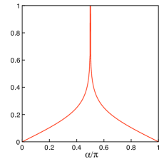
Figure 2: The density $g(\alpha)$ of Lu and Wu [17].

Figure 3: Plots of the scale dependent density $g(\alpha;a)_{N}$ for the Brascamp-Kunz zeros as a function of the angle $\alpha/\pi$ for the $20\times 20$ lattice on the left and the $100\times 100$ lattice on the right. In the first row $a=1,$ in the second row $a=[L^{1/2}]$ and in the third row $a=L=N^{1/2}$. This limiting density (24) of [17] is shown in red.

3.3 Definitions of the density of zeros

In order to recover the result (24) of [17] for $g(\alpha)$ from the partition function zeros of (9) we need to be more precise in the definition of density of zeros. There are two slightly different ways to proceed. We can either divide the circle $s=e^{i\alpha}$ into a set of intervals of equal size and count the number of zeros in each interval or we can compute the size of an interval needed to contain exactly a fixed number of zeros. We here adopt the second method which generalizes (18) by defining

$$g(\alpha;a)=\lim_{N\rightarrow\infty}g(\alpha^{(N)}_{j};a)_{N}$$ (26)

where

$$g(\alpha^{(N)};a)_{N}=\frac{a}{N(\alpha^{(N)}_{j+a}-\alpha^{(N)}_{j})}~{}~{}{\rm with}~{}~{}a=[cN^{p}].$$ (27)

where $[x]$ denotes the integer part of $x$. If $p=0$ and $c=1$ we recover the density definition (18). If the limit exists for some $p_{0}<1$ it will continue to exist for $p>p_{0}$. The quantity $p_{0}$ can be called the scale for which the density exists.

We examine the existence of these limits for the Brascamp-Kunz zeros on the $L\times L$ lattice where $N$ is proportional to $L^{2}$. In Figure 3 we compare for the $20\times 20$ and $100\times 100$ lattices the scale dependent densities for $a=1,~{}a=[L^{1/2}]$ and $a=L=N^{1/2}$. We see for $a=1$ and $a=[L^{1/2}]$ that the limit does not appear to exist but the limit does seem to exist for $a=L=N^{1/2}.$ Further studies reveal that the limit does not exist for $0\leq p<1/2$ but does exist for $1/2<p<1$. However, we have no analytic proof of these numerical observations.

3.4 Dependence on u for $H>0$

When $H>0$ the free energy is no longer invariant under $E\rightarrow-E$ (ie. ferromagnetic $\rightarrow$ antiferromagnetic). However, for Brascamp-Kunz boundary conditions the partition function does remain symmetric under $u\rightarrow-u$ and hence is a polynomial in $u^{2}$. In addition, as the magnetic field $H$ increases the zeros in the $u^{2}$ plane move to infinity as $x=e^{-2H/k_{B}T}\rightarrow 0$ so instead of $u^{2}$ we consider the rescaled variable

$$y=u^{2}x^{1/2}.$$ (28)

We plot the zeros of the Ising partition function with Brascamp-Kunz boundary conditions on the $22\times 22$ lattice for several values of $x$ in Figure 4. These extend the earlier work of Matveev and Shrock [20] on $7\times 8$ lattices with helical boundary conditions and Kim [21] on $14\times 14$ lattices with cylindrical boundary conditions.

Figure 4: Brascamp-Kunz zeros in the plane $y=u^{2}x^{1/2}$ on the $22\times 22$ lattice for values of $x=0.99,~{}0.90,~{}0.50,~{}0.10,~{}0.01,~{}0.0001$.

It is quite clear from these plots that as $H\rightarrow\infty~{}(x\rightarrow 0)$ the zeros become symmetric under $y\rightarrow-y$. This limiting case of the Ising model on the isotropic square lattice is the hard square system at fugacity

$$z=y^{2}$$ (29)

which has been studied in [7] for cylindrical boundary conditions on the $40\times 40$ lattice. We plot these zeros in Figure 5 along with the similar plot for hard hexagons on the $39\times 39$ lattice for comparison.

Figure 5: Comparison in the complex fugacity plane $z$ of the zeros of the partition function with cylindrical boundary of hard squares on the $40\times 40$ lattice to hard hexagons on the $39\times 39$ lattice taken from Figure 2 of ref. [7].

It is strikingly obvious that as $H$ increases from zero that the inner and outer loops in Figure 4 behave in drastically different ways. The inner loop in Figure 4 which separates the disordered from the ferromagnetic ordered phase smoothly becomes the line $-1\leq z\leq z_{d}$ of hard squares whereas the outer loop does not remain a curve and spreads out into a two dimensional area. These two regions must be treated separately.

3.5 The inner loop zeros

To study the inner loop zeros in more detail we plot them on an expanded scale in Figure 6 for a $22\times 22$ lattice.

Figure 6: Partition function zeros for the $22\times 22$ lattice with Brascamp-Kunz boundary conditions on the inner loop in the plane $y=u^{2}x^{1/2}$ for $x=1.0,~{}0.99,~{}0.98,~{}0.95.~{}0.90,~{}0.80$

These plots make it abundantly clear that there is a sharp change in behavior which sets in as soon as $H$ is increased from zero and that this transition has been completed for $x<0.95$. In the region $0.95\leq x<1$ the deviations from a smooth curve become sufficiently large that a one dimensional density formula becomes inappropriate. Furthermore it is likely that the structure in this region will change with increasing lattice size. However, for $x<0.95$ the locus of zeros has become quite smooth and we can consider a density function

$$D(y_{j})=\frac{1}{N|y_{j+1}-y_{j}|}$$ (30)

where $y_{j}$ is the position of the $j^{th}$ zero as measured from the endpoint on the right and $N$ is the number of zeros on the inner loop. We plot this density in Figure 7 versus the index $j$.

Figure 7: The nearest neighbor density of zeros (30) of the $22\times 22$ lattice with Brascamp-Kunz boundary conditions in the plane $y=u^{2}x^{1/2}$ for $x=0.94,~{}0.90,~{}0.80,~{}0.50,~{}0.10,~{}0.01$ versus the the index $j$ .

For $x>0.90$ it is clear from Figure 7 that the nearest neighbor density is not smooth for $L=22$. This connects with the behavior already seen for $H=0$. However, for $x\leq 0.8$ the nearest neighbor density is very smooth except at the rightmost end and the spacing of zeros behaves for large $N$ as $1/N$ which is what was observed for hard squares and hexagons in [7].

Universality suggests that for sufficiently large $N$ the density at the right-hand endpoint should diverge for all $x<1$. This is more or less seen qualitatively in Figure 7 for $x<0.5$ and in the hard square limit an exponent of $1/6$ was estimated in [7] from the data of the $40\times 40$ lattice. However, it is not possible to extract an accurate exponent of divergence from the data shown in Figure 7.

3.6 Outer loop zeros

The zeros on the outer loop behave very differently from the inner loop zeros. Instead of the zeros of $H=0$ changing their spacing to the density function (30) the zeros have spread out into an area which grows as $H$ increases. It may be conjectured that this spreading into an area happens for the entire outer loop but for any finite size lattice there will always be a region near the real axis where this effect cannot be resolved.

3.7 Toroidal and cylindrical boundary conditions

In order to better understand the role on boundary conditions we plot the zeros as a function of $H$ in the $y=ux^{1/4}$ plane for toroidal boundary conditions on the $16\times 17$ lattice in Figure 8 and for cylindrical boundary conditions of the $20\times 20$ lattice in Figure 9.

Figure 8: The zeros in the plane of $y=ux^{1/4}$ for the $16\times 17$ lattice with toroidal boundary conditions for $x=1.0,~{}0.9,~{}0.5,~{}0.1,~{}0.01,~{}0.001.$

Figure 9: The zeros in the $y=ux^{1/4}$ plane for the $20\times 20$ lattice with cylindrical boundary conditions for $x=1.0,~{}0.5,~{}0.1,~{}0.01,~{}0.001,~{}0.0001,~{}0.00001,~{}0.000001.$

For cylindrical boundary conditions the exact partition function on the finite lattice was computed in 1967 [22]. In contrast with Brascamp-Kunz boundary conditions the zeros are not symmetric under $u\rightarrow-u$ and at $u=-1$ the $L\times L$ lattice has an $L$ fold zero. The total number of zeros is $2L^{2}-L$.

As $H$ increases from $H=0$ the $L$ fold zero at $u=-1$ of the $L\times L$ lattice becomes $L$ zeros on the negative axis which for $L$ even are in closely spaced pairs. As $H$ is increased the pairs coalesce and become complex conjugate pairs. For sufficiently large $H$ they are all complex. However, the imaginary part is sufficiently small that in the plots they appear to be on the negative axis.

When $x$ is sufficiently small the three groups of $L$ zeros each tend to infinity at angles $\pi,~{}\pm\pi/3$. This has previously been seen in [21]. We have no explanation for this phenomenon. The remaining $2L^{2}-L-3L$ zeros have a 4-fold symmetry (for L even) at $x\rightarrow 0$.

4 Transfer matrix eigenvalues

An alternative method to compute partition functions is to define a (row to row) transfer matrix on the $L_{v}\times L_{h}$ lattice of size $2^{L_{h}}\times 2^{L_{h}}$. We denote by $T_{C}(L_{h})$ the transfer matrix with periodic boundary conditions in the $L_{h}$ direction and by $T_{F}(L_{h})$ the transfer matrix with free boundary conditions in the $L_{h}$ direction.

In 1949 Kaufman [23] computed all eigenvalues of $T_{C}(L_{h})$ and found that there are two sets

$$\lambda_{+}=\prod_{n=0}^{L_{h}-1}e^{\pm\gamma_{2n+1}}\hskip 14.45377pt\lambda_{-}=\prod_{n=0}^{L_{h}-1}e^{\pm\gamma_{2n}}$$ (31)

with

$$e^{\pm\gamma_{m}}=s+s^{-1}-\cos\phi_{m}\pm\left((s+s^{-1}-\cos\phi_{m})^{2}-1\right)^{1/2}$$ (32)

where $\phi_{m}=\pi m/L_{h}$ and there must be an even number of minus signs. Each set of eigenvalues contains $2^{L_{h}-1}$ eigenvalues.

For all $\gamma_{m}$ for $m\neq 0$ the square roots are defined as positive for $0<T<T_{c}~{}~{}(1<s<\infty)$.

For $|s|=1$ and all $\phi_{m}$ such that $(s+s^{-1}-\cos\phi_{m})^{2}<1$ the modulus of $e^{\pm\gamma_{m}}$ is unity and thus many eigenvalues on the circle $|s|=1$ will have the same modulus.

For $\gamma_{0}$ a factorization occurs under the square root and

$$e^{\gamma_{0}}=s+s^{-1}-1+(s-1)(s^{-2}+1)^{1/2}$$ (33)

So $\gamma_{0}$ is positive for $s>1$ and negative for $s<1$. For $T=T_{c}$ we have $s=1$ and $\gamma_{0}=0$.

There are four constructions of partition functions from these transfer matrices.

• $L_{v}$ periodic, $L_{h}$ periodic

  $$Z^{CC}_{L_{v},L_{h}}={\rm Tr}T_{C}(L_{h})^{L_{v}}=\sum_{k}\lambda^{L_{v}}_{C;k}(L_{h}),$$ (34)

• $L_{v}$ periodic, $L_{h}$ free

  $$Z^{C,F}_{L_{v},L_{h}}={\rm Tr}T_{F}(L_{h})^{L_{v}}=\sum_{k}\lambda^{L_{v}}_{F;k}(L_{h})$$ (35)

• $L_{v}$ free, $L_{h}$ periodic

  $$Z^{FC}_{L_{v},L_{h}}={\bf v}\cdot T_{C}^{L_{v}-1}(L_{h}){\bf v^{\prime}}=\sum_{k}{\bf v\cdot v_{k}}\lambda_{C;k}^{L_{v}-1}{\bf v_{k}\cdot v^{\prime}}$$ (36)

• $L_{v}$ free, $L_{h}$ free

  $$Z^{FF}_{L_{v},L_{h}}={\bf v}\cdot T_{F}^{L_{v}-1}(L_{h}){\bf v^{\prime}}=\sum_{k}{\bf v\cdot v_{k}}\lambda_{F;k}^{L_{v}-1}{\bf v_{k}\cdot v^{\prime}}$$ (37)

where $\lambda_{C;k}$ and $\lambda_{F;k}$ are eigenvalues, ${\bf v}$ and ${\bf v^{\prime}}$ are suitable boundary vectors and ${\bf v_{k}}$ are the eigenvectors.

It is obvious by symmetry that $Z^{CF}_{L_{h},L_{v}}=Z^{FC}_{L_{v},L_{h}}$ and thus the explicit results of 1967 for $Z^{FC}_{L_{v},L_{h}}$ must be obtainable from the eigenvalues of $T_{F}(L_{h})$ but the eigenvalues of $T_{F}(L_{h})$ have never been computed. Clearly something is missing.

4.1 Equimodular curves

The Ising model at $H=0$ and $H/k_{b}T=i\pi/2$ are the only models where the finite size partition function (at arbitrary size) has ever been computed from the transfer matrix eigenvalues. For all other models when there is one eigenvalue $\lambda_{\rm max}$ that is dominant (i.e. of maximum modulus) on the finite lattice the free energy per site in the thermodynamic limit is computed as

$$-F/kT=\lim_{L_{h}\rightarrow\infty}\lim_{L_{v}\rightarrow\infty}\frac{1}{L_{v}L_{h}}\ln\lambda^{L_{v}}_{\rm max}(L_{h}).$$ (38)

However an eigenvalue which is dominant in one portion of the $u=e^{-2E/kT}$ plane will not, in general, be dominant in all parts of the plane. The places where two or more eigenvalues have the same modulus form equimodular curves and can separate the complex $u$ plane into many distinct regions.

When there are only two equimodular eigenvalues $\lambda_{1}(L_{h})$ and $\lambda_{2}(L_{h})$ on the equimodular curve and there are periodic boundary conditions in the $L_{v}$ direction we can approximate the partition function near the curve as

$$Z_{L_{v},L_{h}}\sim\lambda_{1}(L_{h})^{L_{v}}+\lambda_{2}(L_{h})^{L_{v}}$$ (39)

and thus for fixed $L_{h}$ as $L_{v}\rightarrow\infty$ there will be a smooth distribution of zeros with a spacing of $1/L_{v}$ and a density determined by the phase difference between the two eigenvalues [7].

For free boundary conditions we have

$$Z_{L_{v},L_{h}}\sim c_{1}\lambda_{1}(L_{h})^{L_{v}}+c_{2}\lambda_{2}(L_{h})^{L_{v}}$$ (40)

where $c_{j}={\bf(v\cdot v_{j})(v_{j}\cdot v^{\prime})}$

When there are only two equimodular eigenvalues this relation for zeros is sufficient for partition functions computed by first taking $L_{v}\rightarrow\infty$ and then taking $L_{h}\rightarrow\infty$ so that the aspect ratio $L_{h}/L_{v}$ vanishes. For thermodynamics to be valid the free energy must be independent of aspect ratio as long as $0<L_{h}/L_{v}<\infty$.

4.2 Equimodular curves for $T_{C}(L_{h})$ at $H=0$

For the Ising model at $H=0$ the equimodular curves of the transfer matrix $T_{C}(L_{h})$ can be numerically computed from the eigenvalues (31),(32) of Kaufman [23] where we note that the corresponding momentum is

$$P=\sum_{m}\phi_{m}~{}~{}({\rm mod}~{}2\pi).$$ (41)

We plot these curves in the complex $u$ plane in Figures 10 and 11 for $L_{h}=8,10,12$.

Figure 10: The equimodular curves in the $u$ plane for $T_{C}(L_{h})$ for $L_{h}=8$. On the left all eigenvalues are considered and on the right the restriction to the momentum sector $P=0$ is made. The sectors where $\lambda_{+}$ is dominant is marked by $+$ and the sector where $\lambda_{-}$ is dominant is marked by a circle. The multiplicity of the crossings on the curves are indicated by colors. On left panel:red=2, green=3, black=4, blue=8, yellow=16, purple=32, brown=64 On right panel: red=2, green=4, blue=8, brown =3, black=9.

Figure 11: The equimodular curves in the $u$ plane for $T_{C}(L_{h})$ at $P=0$ for $L_{h}=10$ on the left and 12 on the right. Red indicates a multiplicity of 2, green of 4 and blue of 8. For $L=10$ the sequence of multiplicities on the upper (antiferromagnetic) sequence (increasing towards $u=i$) is 2,4,8,4,18,24 and the lower (ferromagnetic) sequence 2,2,4,4,8,8,18,28. For $L=12$ the upper sequence 2,4,8,2,18,18,52,84 and the lower sequence is 2,2,4,4,8,8,18,26,52,88

These curves have the following striking properties:

1. All eigenvalues are equimodular at $u=\pm i$.

2. The equimodular curves in the $u$ plane of the eigenvalues $\lambda_{+}$ and the eigenvalues $\lambda_{-}$ are segments of the two circles $u=\pm 1+2^{1/2}e^{i\theta}$ which is the curve on which there are Brascamp-Kunz zeros.

3. On most of the segments of this curve there are more than two equimodular eigenvalues.

4. The equimodular curves formed by one eigenvalue $\lambda_{+}$ and one $\lambda_{-}$ do not lie on the curve of Brascamp-Kunz zeros.

The multiple degeneracies on the equimodular curves destroy the mechanism for a smooth density of zeros of the $L_{v}=L_{h}=L$ lattice with a $1/L^{2}$ spacing. The mechanism which changes the scale of smooth zeros from $1/L^{2}$ to $1/L$ seen in section 3.3 is not understood.

4.3 $u$ plane eigenvalues for $x=0.99$

When $H$ is increased from $H=0$ the transfer matrix eigenvalues have been computed numerically. In Figure 12 we plot the equimodular curves for all eigenvalues for $x=0.99$. (We note that the curves extending from the upper branch to infinity are also present for $H=0$ but are not seen in Figure 10 because in that figure the imaginary part of $u$ is restricted to $0\leq\mathrm{Im}(u)\leq 1$.)

Figure 12: Equimodular curves in the $u$ plane for $x=0.99$ of $T_{C}(L_{h})$ for $L_{h}=6$ on the left and $L_{h}=8$ on the right. Red is for singlet-singlet crossings, green is for singlet-doublet and blue is for doublet-doublet

By comparing Figure 12 with Figures 10 and 11 we see that several dramatic phenomena occur for $H>0$.

1. For $H>0$ the rays to the imaginary axis very rapidly retreat into the curve of the Brascamp-Kunz zeros. This is caused by the lifting of the near degeneracy of eigenvalues in the $\lambda_{+}$ and $\lambda_{-}$ subspaces of $H=0$. The larger $L_{h}$ the more rapid the retreat.

2. The rays to infinity separate regions of $P=0$ and $P=\pi$ and are virtually unchanged for $H>0$.

3. The multiple degeneracies disappear. For momenta $P=0,\pi$ the eigenvalues are singlets for $P\neq 0,~{}\pi$ the momenta $\pm P$ are doubly degenerate. In Figure 12 all singlet-doublet and doublet-doublet curves enclose regions where the dominant eigenvalue has $P\neq 0,\pi$ but for $x=0.99$ some of the regions are too small to be observed as areas.

In Figure 13 we plot for $L_{h}=8$ the region near $u=i$ in more detail. Thus far eigenvalues for $L_{h}\geq 10$ have not been computed for the case $H\neq 0$.

Figure 13: Equimodular curves in the $u$ plane for $x=0.99$ expanded near $u=i$ for $T_{c}(L_{h})$ with $L_{h}=8$. Red is for singlet-singlet crossings, green is for singlet-doublet and blue is for doublet-doublet

5 An interpretation

It is very clear, both from the behavior of the partition function zeros and the degeneracy of the equimodular curves, that there is a drastic qualitative difference between $H=0$ and $H\neq 0$. We conjecture here an interpretation of the singularities (11) found by Nickel [1, 2] based on this behavior. The argument is substantially different for the inner (ferromagnetic) and outer (antiferromagnetic) loops in the $u$ plane. Naturally conjectures concerning analyticity based solely on finite size computations can only be suggestive.

5.1 Scenario on the ferromagnetic loop

We conjecture that on the ferromagnetic loop for $H>0$ the zeros approach a curve as $L_{h}L_{v}=N\rightarrow\infty$ and that for sufficiently large $N$ and fixed $H\neq 0$ the limit

$$\lim_{N\rightarrow\infty}N(u_{j+1}-u_{j})<\infty$$ (42)

exists. However, this cannot be uniform in $H$ and thus the limits $H\rightarrow 0$ and $N\rightarrow\infty$ will not commute. For both $H=0$ and $H\neq 0$ the free energy is analytic at the locus of zeros. However, for $H\neq 0$ the analytic continuation beyond the zero locus encounters many singularities which accumulate in the limit $H\rightarrow 0$ to the singularities of Nickel (11). The location (and nature) of these singularities is different if the continuation is from the interior (low temperature) or exterior (high temperature) of the loop. The amplitude of the singularities vanishes as $H^{2}$ at $H\rightarrow 0$ and hence the analyticity of the free energy at $H=0$ is maintained.

In this scenario the singularities in the susceptibility at $|s|=1$ occur because taking two derivatives with respect to $H$ kills the $H^{2}$ in the amplitude of the singularities but does not move the locations.

It can be argued that the non-integrability of the Ising model at $H\neq 0$ is caused by these singularities in the analytic continuation beyond the locus of zeros. Nevertheless, there are no singularities on the locus of zeros except at the endpoints. The singularity at the endpoint is expected [7] to have the same behavior as the endpoint behavior of hard squares, hard hexagons and the Lee-Yang edge.

We may now make contact with the scenario of Fonseca and Zamolodchikov [4] who assume that in the field theory limit the free energy may be continued far beyond the locus of zeros. The field theory limit is defined by $T\rightarrow T_{c}$ and $H\rightarrow 0$ such that

$$\tau=(T-T_{c})H^{-8/15}$$ (43)

is fixed of order one. In terms of this scaled variable Fonseca and Zamolodchikov posit that there is analyticity across the locus of zeros and that there is an extensive region of analyticity in the analytically continued free energy which sees none of the singularities which, in this interpretation, produce the singularities of Nickel. The analyticity of [4] will be consistent with our scenario if the singularities which approach the point $u={\sqrt{2}}-1$ as $H\rightarrow 0$ is slower than the scaling $H^{8/15}$. If this is indeed the case then there is no contradiction between the field theory computations of [4] and the singularities of [1, 2].

5.2 Scenario on the antiferromagnetic loop

The behavior on the antiferromagnetic loop is quite different from the behavior on the ferromagnetic loop because now the zeros spread out into areas for $H\neq 0$. Moreover the pinching of the zeros at the antiferromagnetic singularity at $u={\sqrt{2}}+1$ remains a pinch for all values of $x$ and furthermore the singularity in the free energy in the hard square limit is numerically estimated from high density series expansions [24, 25] to be the same as the logarithmic singularity at $T_{c}$ of the antiferromagnetic Ising model at $H=0$.

The zeros in Figures 4 and 5 do appear to be smoothly spaced in a two dimensional region so from this point of view the distribution of zeros which for $H=0$ was studied in section 3.3 has moved smoothly from the circle to an area in the plane. There is, unfortunately, not sufficient data to conjecture the behavior where the zeros in the $N\rightarrow\infty$ limit pinch the positive $u$ axis. Even in the hard square limit it cannot be concluded from Figure 5 if the zeros pinch as a curve, as a cusp with an opening angle of zero or as a wedge with a nonzero opening angle. The field theory argument of [4] does not extend to the hard square limit and it is not obvious how to consider analytic continuation into an area of zeros.

The second feature which needs an explanation is the approach of the zeros to the hard square limit in both Figure 4 for Brascamp-Kunz boundary condition in the $y=u^{2}x^{1/2}$ plane and in Figures 9 and 8 for cylindrical and toroidal boundary conditions in the $y=ux^{1/4}$ plane. Namely the emergence of the 2 fold symmetry for Brascamp-Kunz and the 4 fold symmetry for cylindrical and toroidal boundary conditions. For all boundary conditions new points of singularity are created in the complex $y$ plane as $H$ is increased, which in the hard square limit become identical with the singularity on the positive $y$ axis. The mechanism for the creation of these new points of singularity is completely unknown.

5.3 The bifurcation points

However, perhaps the most striking feature of the zeros is the existence of the special points where the one dimensional locus bifurcates into the two dimensional area. It is the existence of these points which allows us to use the terms ferromagnetic and antiferromagnetic branch. At $H=0$ these points are at $u=\pm i$ where all eigenvalues are equimodular and the free energy is singular [20]. In the hard square limit this point is at $z=-1$ where all eigenvalues are also equimodular [26]. It is natural to conjecture that for all values of $H$ the free energy fails to be analytic at these points.

6 Conclusion

In this paper we have presented the results of extensive numerical computations of the zeros of the partition function of the Ising model in a magnetic field $H$ and a companion study of the dominant eigenvalues of the transfer matrix as $H$ goes from $H=0$ to the hard square limit $H\rightarrow\infty$. This reveals that in the ferromagnetic region the distribution of zeros changes radically when $H$ is infinitesimally increased from $H=0$ and this feature is used to give an interpretation of the natural boundary in the magnetic susceptibility conjectured by Nickel [1, 2] which is consistent with the analyticity of the scaling limit assumed by Fonseca and Zamolodchikov [4]. However, an analytic argument for this scenario remains to be found and further data is needed in order to reliably understand the approach to the hard square limit.

References

References

- [1] B.G. Nickel, On the singularity structure of the 2D Ising model susceptibility, J. Phys. A 32 3889–3906 (1999).
- [2] B.G. Nickel, Addendum to ‘On the singularity structure of the 2D Ising model susceptibility’, J. Phys. A 33 1693–1711 (2000).
- [3] A.J. Guttmann and I.G. Enting, Solvability of some statistical mechanical systems, Phys. Rev. Lett. 76, 344-346 (1996).
- [4] P. Fonseca and A. Zamolodchikov, Ising field theory in a magnetic field: analytic properties of the free energy, J. Stat. Phys. 110 527–590 (2003).
- [5] V.V. Mangazeev, M.Yu. Dudalev, V.V. Bazhanov, M.T. Batchelor, Scaling and universality in the two-dimensional Ising model with a magnetic field, Phys. Rev. E 81 060103(R) (2010).
- [6] V.V. Mangazeev, M.T. Batchelor, V.V. Bazhanov, M.Yu. Dudalev, Variational approach to the scaling function of the 2D Ising model in a magnetic field, J. Phys. A 42 042005 (2009).
- [7] M. Assis, J.L. Jacobsen, I. Jensen, J-M. Maillard and B.M. McCoy, Integrability vs non-integrability; hard hexagons and hard squares compared, J. Phys. A 46 445208 (2013).
- [8] H.J. Brascamp and H. Kunz, Zeros of the partition function for the Ising model in the complex temperature plane, J. Math. Phys. 15 65-66 (1974).
- [9] L. Onsager, Crystal statistics I. A two-dimensional model with an order-disorder transition, Phys. Rev. 65 117-149 (1944).
- [10] T.D. Lee and C.N. Yang, Statistical theory of equations of state and phase transitions II, Phys. Rev. 87 410-419 (1952).
- [11] P.J. Kortman and R.B. Griffiths, Density of zeros on the Lee-Yang circle for two Ising ferromagnets, Phys. Rev. Lett. 27 1439-1442 (1971).
- [12] R.J. Creswick and S-Y. Kim, Finite-size scaling of the density of zeros of the partition function in first and second order phase transitions, Phys. Rev. E 56 2418-2422 (1997).
- [13] S-Y. Kim, Density of Lee-Yang zeros for the Ising magnet, Phys. Rev. E 74 011119 (2006).
- [14] C.N. Yang. The spontaneous magnetization of the two dimensional Ising model, Phys. Rev. 85 808-816 (1952).
- [15] B.M. McCoy and T.T. Wu, Theory of Toeplitz determinants and the spin correlations of the two dimensional Ising model II, Phys. Rev. 155 438-452 (1967).
- [16] J.S. Langer, Theory of the condensation point, Annals Phys. 41 108-157 (1967); Annals Phys. 281 941-990 (2000).
- [17] W.T. Lu and F.Y. Wu, Density of Fisher zeros for the Ising model, J. Stat. Phys. 102 953-970 (2001).
- [18] D.A. Bini and G. Fiorentino, Design, analysis and implementation of a multiprecision polynomial rootfinder, Numer. Algorithms 23 127–173 (2000). MPSolve is available from http://numpi.dm.unipi.it/software/mpsolve
- [19] S. Fortune, An iterated eigenvalue algorithm for approximating the roots of univariate polynomials, J. Symb. Comput. 33 627–646 (2002). Eigensolve is available from http://ect.bell-labs.com/who/sjf/eigensolve.html
- [20] V. Matveev and R. Shrock, Complex-temperature properties of the two-dimensional Ising model for nonzero magnetic field, Phys. Rev. E 53 254-267 (1996).
- [21] S-Y Kim, Fisher zeros of the Ising antiferromagnet in an arbitrary nonzero magnetic field, Phys. Rev. E 71 017102 (2005).
- [22] B.M. McCoy and T.T. Wu, Theory of Toeplitz determinants and the spin correlations of the two dimensional Ising model IV, Phys. Rev. 162 436-475 (1967).
- [23] B. Kaufman, Crystal statistics II. Partition function evaluated by spinor analysis, Phys. Rev. 76 1232-1243 (1949).
- [24] R.J. Baxter, I.G. Enting and S.K. Tsang, Hard square lattice gas, J. Stat. Phys. 22 465-489 (1980).
- [25] G. Kamieniarz and W. Blöte, The non-interacting hard-square lattice gas: Ising universality, J. Phys. A 26 6679-6689 (1993).
- [26] P. Fendley, K. Schoutens and H. van Eerten, Hard squares with negative activity, J. Phys. A 38 315-322 (2005).