A Galactic Molecular Cloud Clump Catalog from Hi-GAL Data: Method and Initial Results Comparison to BGPS

Abstract

As the precursors to stellar clusters, it is imperative that we understand the distribution and physical properties of dense molecular gas clouds and clumps. Such a study has been done with the ground-based Bolocam Galactic Plane Survey (BGPS). Now the Herschel infrared GALactic plane survey (Hi-GAL) allows us to do the same with higher quality data and complete coverage of the Galactic plane. We have made a pilot study comparing dense molecular gas clumps identified in the Hi-GAL and BGPS surveys, using six $2^{\circ}\times 2^{\circ}$ regions centered at Galactic longitudes of $\ell=11^{\circ}$, 30^∘, 41^∘, 50^∘, 202^∘, and $217^{\circ}$. We adopted the BGPS methodology for identifying clumps and estimating distances, leading to 6198 clumps being identified in our substudy, with 995 of those having well-constrained distances. These objects were evenly distributed with Galactic longitude, a consequence of Hi-GAL being source confusion limited. These clumps range in mass from 10^-2 M_⊙ to 10⁵ M_⊙, and have heliocentric distances of up to 16 kpc. When clumps found in both surveys are compared, we see that distances agree within 1 kpc and ratios of masses are of order unity. This serves as an external validation for BGPS and instills confidence as we move forward to cataloging the clumps from the entirety of Hi-GAL. In addition to the sources that were in common with BGPS, Hi-GAL found many additional sources, primarily due to the lack of atmospheric noise. We expect Hi-GAL to yield $2\times 10^{5}$ clumps, with 20% having well-constrained distances, an order of magnitude above what was found in BGPS.

1 Introduction

Significant observational and theoretical progress has been made in the study of star formation. However, crucial aspects, such as why the stellar and star cluster initial mass functions appear uniform across many Galactic environments, remain unexplained. In order to understand stellar clusters and OB associations, it is critical to understand that from which they are formed. Thus the study of molecular cloud clumps has become a primary focus in the field of high-mass star formation (e.g., McKee & Ostriker, 2007). Large-scale studies of the Galactic dense molecular gas — its distribution and properties — are necessary in order to challenge models of galaxy evolution and reveal the origin of the stellar cluster initial mass function.

Such large-scale studies have recently become practical with the actualization of Galactic Plane dust continuum surveys at sub/millimeter wavelengths [BGPS: Aguirre et al. (2011); Ginsburg et al. (2013); ATLASGAL: Schuller et al. (2009); Csengeri et al. (2014, 2016); Hi-GAL: Molinari et al. (2010, 2016)]. These surveys have detected tens of thousands of molecular cloud clumps and cores, which can now be extracted and used to study physical properties of high-mass star formation regions. The census of Galactic dense molecular cloud structures enabled by these surveys will constrain star formation and galaxy evolution theories (e.g., Kennicutt & Evans, 2012). Such studies of physical properties (e.g., Peretto & Fuller, 2010; Giannetti et al., 2013; Elia et al., 2013) and mass distributions (e.g., Netterfield et al., 2009; Olmi et al., 2013, 2014; Gómez et al., 2014; Ellsworth-Bowers et al., 2015; Wienen et al., 2015) have begun, but have yet to reveal a coherent story concerning the evolution of the dense interstellar medium and the uniformity of the stellar cluster mass function.

Fortunately, theoretical models of the dense interstellar medium are beginning to produce predictions robust enough to be used in conjunction with observational data to constrain the molecular cloud clump mass function (e.g., Donkov et al., 2012; Veltchev et al., 2013). This function is generally expected to take either a power-law or lognormal form, with each distribution corresponding to a different physical process in the molecular clouds. Gravitational collapse of dense structures would produce a power-law (e.g., Padoan & Nordlund, 2002). A lognormal density distribution can be produced by supersonic turbulence (e.g., Padoan et al., 1997), although such conditions are not necessary (Tassis et al., 2010). Likely, these processes are interacting within the dense molecular clouds, producing a mass function displaying a combination of these forms (e.g., Offner et al., 2014; Hopkins, 2013). Which mode dominates will have implications for the competing theories of high-mass star formation (Elmegreen, 1985).

On a grander scale, the distribution of dense molecular gas in the Milky Way has implications for using our Galaxy as the ground truth for studies of galaxy evolution. Until recently, numerical models had substantial difficulty generating long-lived spiral galaxies. This was due either to rapid depletion of gas before the disks could be sustained or the galaxies blowing themselves apart with an inadequate balance of gravity and stellar feedback. In the past two decades, remarkable progress has been made towards reproducing observed properties of galaxies (e.g., Katz et al., 1996; Kereš et al., 2009; Stinson et al., 2013). Currently, simulations that incorporate feedback into the interstellar medium from star formation and the late stages of massive stellar evolution can reliably create large spiral galaxies. However, the star formation, being unresolved in the simulations, uses prescriptive recipes tuned a posteriori. Typically, star formation is turned on at a fixed interstellar medium density threshold (e.g. $10^{3}$ cm^-3), at which point $\sim 1\%$ of the gas mass is converted into stars (Kim et al., 2014). Unfortunately, numerical simulations have largely been unable to a priori produce the strong winds and inefficiency of star formation observed in galaxies (Hopkins et al., 2014). The dense molecular gas distribution is an observational key to probing the star formation efficiency on scales resolvable by simulations. Because the amount and rate of star formation drives feedback, it is imperative that these recipes are tested against reality.

We will use the Herschel Space Observatory’s Hi-GAL survey, which provides complete coverage of the Galactic Plane in the far-infrared to submillimeter wavebands, to create such a map and test these explanations of clump mass functions and galaxy evolution models. This paper describes the method we will be using to identify Hi-GAL molecular cloud clumps and determine their heliocentric distances. It will furthermore compare the results of a number of representative test regions to BGPS, a well-vetted benchmark. However, we expect Hi-GAL to significantly supersede BGPS. Molinari et al. (2016) have independently begun cataloging the dense molecular cloud clumps found in the Hi-GAL survey. They have identified and extracted photometry for clumps found in the majority of the inner Galaxy in all five of Herschel’s photometric bands. This work serves as a complement to the work of Molinari et al. (2016) through the use of a fundamentally different source identification technique. In addition, we go beyond their work in the determination of distances and physical properties of the clumps.

Dense molecular gas structures can be divided into three categories: clouds, clumps, and cores. Molecular clouds have denser substructures called molecular cloud clumps, which in turn have even denser substructures called molecular cloud cores. These cores are gravitationally bound and will form individual stars or simple stellar systems. Typical radii are clouds $R=1-7.5$ pc, clumps $R=0.15-1.5$ pc, and cores $R=0.015-0.1$ pc. Typical densities are clouds $50-500$ cm^-3, clumps $10^{3}-10^{4}$ cm^-3, and cores $10^{4}-10^{5}$ cm^-3 (Bergin & Tafalla, 2007). Cores are only resolvable within a couple kiloparsecs by single-dish telescopes. Clumps are detectable within $\sim 7$ kpc, beyond which the resolution is no longer sufficient for Herschel. Farther out we can only resolve entire clouds (Dunham et al., 2011).

2 Data

Previously, the Bolocam Galactic Plane Survey (BGPS) was made with the Caltech Submillimeter Observatory and was released in two versions (Aguirre et al., 2011; Ginsburg et al., 2013). BGPS was a $\lambda=1.1$ mm survey over the longitudes $-10^{\circ}<\ell<90^{\circ}$ and latitudes $|b|<0.5^{\circ}$, plus an additional 20 deg². From the survey, a catalog of 8,594 (Version 2) sources was produced, 20% of which have well constrained distances. Even with its incomplete coverage of the Galactic Plane, BGPS showed the emergence of spiral arms, as well as evidence for significant amounts of dense interarm gas (Ellsworth-Bowers et al., 2015).

The Herschel infrared GALactic plane survey (Hi-GAL) (Molinari et al., 2010) originally planned to observe a $2^{\circ}$ strip covering $|\ell|<60^{\circ}$, but was extended to include the entire $360^{\circ}$ of the Galactic plane. Using the SPIRE (Griffin et al., 2010) and PACS (Poglitsch et al., 2010) instruments aboard the Herschel Space Observatory (HSO), this survey observed in wavebands at 70, 160, 250, 350, and 500 $\mu$m. SPIRE (250, 350, and 500 $\mu$m) observed thermal dust emission, which is concentrated in dense molecular gas clumps, whereas PACS (70 and 160 $\mu$m) observed dense gas and extended warm structures to a greater extent than the longer-wavelength SPIRE bands. Owing to the low optical depth of thermal dust in the submillimeter continuum, Hi-GAL allows us to view dense molecular gas throughout the entire Galactic disk. The flux density-limited gas mass sensitivity is 250 M_⊙ ($5\sigma$) at distances up to 20 kpc (corresponding with a $1\sigma$ RMS of 100 mJy at 250 $\mu$m, assuming a temperature of 20 K).

In this paper, we analyzed a representative sample of six Hi-GAL regions, centered at $\ell=11^{\circ}$, 30^∘, 41^∘, 50^∘, 202^∘, and $217^{\circ}$. This sample includes regions from both inner and outer portions of the Galaxy, and, with the exception of $\ell=202^{\circ}$, have a significant overlap with BGPS observations. Figure 1 shows the maps for the $\ell=30^{\circ}$ and 217^∘ regions. Emission levels vary strongly depending on proximity to the Galactic center, but there is extensive structure in all regions.

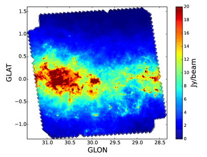
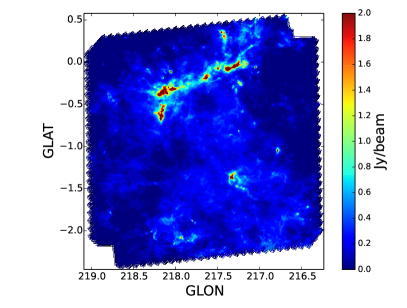
Figure 1: Example maps in SPIRE 500 $\mu$m from our representative sample of Hi-GAL — $\ell=30^{\circ}$ (left), which looks through the edge of the Galactic bar, and $\ell=217^{\circ}$ (right). Emission levels are significantly higher in the inner Galaxy than the outer Galaxy due both to the greater quantities of molecular gas, and to the longer optical path integrating more emission.

3 Method

3.1 Map Making

The Hi-GAL observations are stored in the Herschel Science Archive (HSA) and the Herschel Interactive Processing Environment (HIPE) allows users to access the data. The tool UniHIPE was used to format the HSA data suitable to be input into the Hi-GAL mapping pipeline, Unimap (Piazzo et al., 2012, 2015a, 2015b).

Each Hi-GAL observation is composed of two orthogonal scans. Unimap takes the time-ordered bolometer data from each scan and combines them to make a single astrophysical map, along with various evaluation maps. The pipeline begins by cleaning the time-ordered data. It removes the offset in the input data, then finds and removes signal jumps and glitches, both of which can be caused by cosmic rays. Finally, the drift, a low frequency signal due to slowly varying bolometer temperatures, is fit and removed. The time-ordered data are then made into a map, using an iterated Generalized Least Squares method. This method often leads to cross-like artifacts on bright sources, which are removed by Unimap’s post-processing.

3.2 Filtering

The 500 $\mu$m SPIRE band has the lowest resolution of the bands, with a beam FWHM of $32\arcsec.2$, and so we convolved and rebinned all maps to 500 $\mu$m resolution to enable multiband photometry. Foreground cirrus clouds are present in all of the maps. Since this undesirable flux density is present on angular scales larger than that of molecular cloud clumps, the maps were high-pass filtered on the $3\arcmin$ scale to remove this flux density. The filtering was done in frequency-space using an inverted 2D Gaussian window with $\sigma$ corresponding to $3\arcmin$. This scale was chosen for two reasons. Firs t, it is a larger angular scale than the largest of the BGPS clumps. Second, when the Hi-GAL maps were filtered on a larger scale of $\sigma=5\arcmin$, nearly all of the clumps found were smaller than $3\arcmin$. Thus, this filtering scale removes as much extended emission as possible with minimal attenuation of molecular cloud clump sizes and flux densities (and therefore inferred masses).

Simulations were performed in order to quantify the effects of the high-pass filter. Synthetic Gaussian objects were inserted onto both the $\ell=30^{\circ}$ map, and onto constant background maps. Synthetic sources were distributed randomly, but were restricted to have their centers no closer than three times the source FWHM. The maps were then filtered and objects identified by Bolocat (See Section 3.3) on the constant background map. These source masks were then used to calculate source properties on synthetic sources from the $\ell=30^{\circ}$ background map. This was done for filtering scales of $\sigma=2.4\arcmin$, $3.2\arcmin$, $4.1\arcmin$, and $4.8\arcmin$, and with various synthetic source sizes. For each combination of filtering scale and source size $\sim$1000 sources were generated, using multiple maps where necessary.

Figure 2 shows median attenuation factors (ratios of post-filtering recovered quantities to input quantities) for integrated flux density ($S$), peak flux density ($S_{\text{pk}}$), and FWHM. Our mean clump size corresponds most closely to the second smallest synthetic object size ($1.2\arcmin$), and 90% of our objects are smaller than the dashed line. Thus Hi-GAL clumps will have their integrated flux density attenuated by $(20\pm 10)\%$ for our choice of a filtering scale of $\sigma=3\arcmin$. Similarly, peak flux density will be attenuated by $<1\%$, and FWHM will be attenuated by $(4\pm 3)\%$.

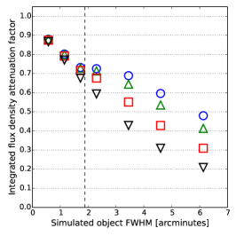
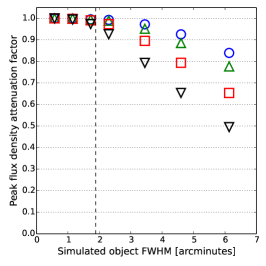
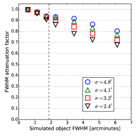
Figure 2: Attenuation factors for integrated flux density (left), peak flux density (center), and FWHM (right). Maps of simulated objects are filtered at various spatial scales. Plotted are the median attenuation factors of objects identified by Bolocat. The dashed line indicates the 90${}^{\text{th}}$ percentile in angular size for objects in our Hi-GAL substudy.

While the majority of the observation regions are covered by both of Herschel’s orthogonal scans, the edges are not. We mask off the regions which are not covered by both scans to exclude these lower-quality data and to avoid confusing the clump-finding code with the original ragged map edges. This removed 29% of flux-containing pixels. We also masked off regions where the high-pass filter added flux density, as opposed to removing it. This was a consequence of the flux density on large scales being negative in these areas, and thus subtracting those negative values added flux density to the pixels. These areas were located at high galactic latitude, where flux density was low. This removed an additional $3-7$%, depending on the field, of flux-containing pixels. The masking process is demonstrated in Figure 3.

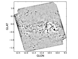
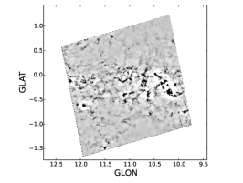
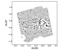
Figure 3: Masking the $\ell=11^{\circ}$ region. Left: The complete high-pass filtered map. The two scan directions can be seen. Center: Pixels not covered by both scans have been masked off. Right: Pixels to which the high-pass filter added flux density have been masked off.

3.3 Source Identification

Source identification was done on 500 $\mu$m SPIRE maps using Bolocat, a seeded watershed algorithm tool developed for BGPS (Rosolowsky et al., 2010). Clumps are found by first identifying regions of significant emission, where significance is determined in units of the local noise estimate. These regions of high significance are then expanded into adjacent lower significance areas, eliminating artificial small-scale structure. Finally, regions are split into multiple clumps, where appropriate, based on local maxima.

Hi-GAL is confusion limited by cirrus, large-scale structure, and source confusion that in BGPS were attenuated by an atmospheric subtraction algorithm. The flux density level of clumps which we can identify in each map is limited by the emission levels in the map. This is demonstrated in the power spectral densities (PSDs) in Figure 4. There is greater power along lines of sight with more interstellar medium (ISM), as well as greater power on larger scales, which may be due to source confusion or the sizes of GMCs themselves. A typical GMC with a radius of 10 pc (e.g. Solomon et al., 1987) would have to be $>23$ kpc away in order to have a 3$\arcmin$ extent.

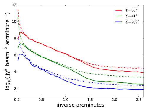
Figure 4: The PSDs for a representative sample of regions. Pre- and post-filtering are shown as dashed and solid lines, respectively. Emission levels on all spatial scales decrease with distance from the Galactic center and lines of sight through the inner Galaxy have greater integrated flux density than towards the outer Galaxy.

With more overall emission in regions nearer the Galactic center, sources in those regions must be brighter for us to detect them above the confusion noise. Therefore we used a constant-noise map for each region, with each “noise” map’s value determined by the emission level in its respective emission map. This was done by fitting the distribution flux densities of pixels with positive emission to an exponential function. The noise value was taken to be proportional to the scale factor of the exponential fit, specifically $0.25\lambda$, where $\lambda$ is the scale factor. As an objective choice was not possible, this selection was made as it consistently produced object contours which matched our visual expectations across regions at widely varying Galactic longitudes. The specific value of $0.25\lambda$ for the noise was chosen after an exploration of Bolocat’s parameter space, which was done using the $\ell=41^{\circ}$ region as a test map.

The threshold for detection and the level down to which areas meeting the detection threshold were expanded were determined first. We chose to set the threshold at $3\sigma$ and to expand down to $1\sigma$, where $\sigma$ is the “noise” level. These values were chosen as they successfully included the flux density which had the appearance of real structure. A division criterion of $2\sigma$ was then decided upon. That is, if the saddle between two local maxima is different from the maxima by at least $2\sigma$, then the clump is divided. This was chosen as it produced results consistent with what was seen in the flux density contours of the test map, a sample section of which can be seen in Figure 5. The initial threshold and division criterion were the same in BGPS, which only expanded down to $2\sigma$.

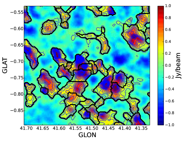
Figure 5: Subsection of the test map for determining Bolocat parameters. Thick black contours show object borders. Thin blue contours show flux density levels with a step size of $2\sigma$, starting at zero.

Choosing a higher threshold would have decreased the number of sources found, as would have choosing a higher floor down to which to expand the regions, since clumps must be at least a beam in size. A higher expansion floor would have also decreased the size of clumps, particularly further from the mid-plane, where flux density is lower. Choosing a lower threshold for splitting clumps would also have led to smaller clumps, although clumps sizes would be limited by the requirement that local maxima must be separated by at least two beam widths. Our choices for these parameters were chosen to match our visual expectations in the test map, attempting to err on the side of a higher detection threshold and less clump division.

The high-pass filter also has associated systematic effects. A more aggressive filter would have resulted in smaller clumps. More significantly, the high-pass filter affects the flux densities of the identified clumps. Figure 6 compares high-pass filtered and unfiltered flux densities in the $\ell=50^{\circ}$ region. Clumps were identified in the filtered map, with photometry re-calculated using the unfiltered maps for the comparison. Photometry was done by summing the flux density found in the pixels within the source boundary, as opposed to background-subtracted aperture photometry. No clump exceeds a flux density ratio of unity by construction, as the small percentage of pixels where the filter added flux density were excluded from source finding.

There is a trend towards the clump containing a higher fraction of the total flux density along the line of sight for higher flux density clumps. On the other hand, the faintest clumps have a wide range of flux density ratios. These trends are seen in all of the regions in this substudy.

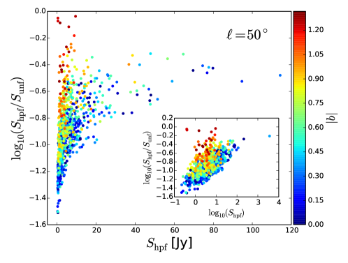
Figure 6: Comparison of high-pass filtered and unfiltered flux densities for the $\ell=50^{\circ}$ region. $S_{\text{hpf}}$ is the clump’s total flux density, taken from the high-pass filtered map in which it was identified, and $S_{\text{unf}}$ is the total flux density in the unfiltered map which lies within the clump’s border. Colors correspond to absolute value of Galactic latitude.

3.4 Distance Determination

This distance determination method was developed for BGPS by Ellsworth-Bowers et al. (2013) and Ellsworth-Bowers et al. (2015), and resulted in 1,710 well-constrained distances. Full details of the method are available in Ellsworth-Bowers et al. (2013, 2015), and a summary is provided here. To construct a 3D map from the sources identified in Hi-GAL and to compute their physical properties, heliocentric distances must be determined. Every line of sight has a function $V_{r}(d_{\odot})$, found from a Galactic rotation curve, describing radial velocity as a function of heliocentric distance. Kinematic distances can be determined by matching a clump’s $v_{\text{LSR}}$ to $V_{r}(d_{\odot})$. However, within the inner Galaxy, this information results in two possible kinematic distances and an ambiguity as to which is the true distance. This ambiguity will be broken using probabilistic methods in a Bayesian framework. A unique distance probability density function (DPDF) will be calculated for each source. The posterior DPDF is found by

$$\text{DPDF}=\mathcal{L}(d_{\odot}|\ell,b,v_{\text{LSR}})\prod_{i}P_{i}(d_{\odot}|\ell,b),$$ (1)

where $\mathcal{L}(d_{\odot}|\ell,b,v_{\text{LSR}})$ is the kinematic distance likelihood, and the $P_{i}(d_{\odot}|\ell,b)$ are various Bayesian priors which will help determine which distance has the higher probability of being true. Once DPDFs are calculated, they can be drawn from in Monte Carlo simulations, even when distances are not well constrained, and thus cloud clump properties can be characterized, with robust uncertainties.

The rotation curve from the Reid et al. (2014) BeSSeL survey, derived from maser parallax measurements to sites of high-mass star forming regions ($\mathbf{-12^{\circ}\leq\ell\leq 240^{\circ}}$), was paired with line-of-sight velocities derived from the ${}^{13}\text{CO}$ Galactic Ring Survey (GRS) to determine the kinematic distances to the molecular cloud clumps. Because there are often multiple velocity components in GRS spectra, each source spectrum is created by subtracting the spectrum of an off-source region from that of the on-source region. The off-source region is determined by creating a rind around the source mask, then excluding pixels associated with other Hi-GAL sources. In this way we eliminate the velocity components not associated with the clump from the clump’s spectrum (see Ellsworth-Bowers et al., 2015, Section 4). Dense gas tracer observations of specific sources, originally made for BGPS, were also utilized. These observations were associated with the new Hi-GAL sources through the object masks obtained from Bolocat. The most powerful $P_{i}$ implemented in BGPS used absorption by the clumps of diffuse Galactic mid-infrared emission near $\lambda=8$ $\mu$m. When the majority of this diffuse emission lies in the background, the molecular cloud clump is called an infrared dark cloud (IRDCs) (Perault et al., 1996; Simon et al., 2006; Peretto & Fuller, 2009; Battersby et al., 2011). Ellsworth-Bowers et al. (2013) defined the term 8 $\mu$m absorption feature to include molecular cloud clumps which exhibit any $\lambda=8$ $\mu$m intensity decrement, thus allowing for absorption less pronounced than seen in IRDCs. The $P_{i}$ developed to take advantage of this feature uses the Galactic infrared emission model of Robitaille et al. (2012) to simulate clumps at various heliocentric distances. These simulated images are then compared to the corresponding GLIMPSE (Churchwell et al., 2009) IRAC Band 4 image, using a $\chi^{2}$ statistic, to generate the $P_{i}$.

The EMAF morphological matching of synthetic GLIMPSE based on Hi-GAL flux density and actual GLIMPSE maps works far better with high-pass filtered maps than with unfiltered maps. In the unfiltered maps, the presence of cirrus emission contributes too much flux to the clumps, causing them to be placed much further away than is plausible. Use of a $\sigma=3\arcmin$ Gaussian high-pass filter removes the cirrus emission and remedies this problem. Two examples from the $\ell=41^{\circ}$ region are shown in Figure 7.

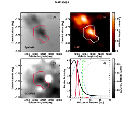
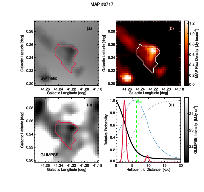
Figure 7: Two examples of EMAF morphological matching in the $\ell=41^{\circ}$ region. Panels (a) on the left and right show the synthetic GLIMPSE map based on the SPIRE 500 $\mu$m map shown in the (b) panels. The synthetic maps shown are the best match to the GLIMPSE map shown in panels (c). Pixels with 8 $\mu$m emission instead of absorption were excluded from the morphological matching. DPDFs are shown in panels (d), with black and red corresponding to EMAF and posterior DPDFs, respectively.

Three additional $P_{i}$s were developed by Ellsworth-Bowers et al. (2013). First, the molecular hydrogen (H₂) uses the small scale height of molecular gas in the disk to constrain clumps at high latitudes to be at their near kinematic distances. This is done using the three-dimensional model of the distribution of molecular gas in the disk of Wolfire et al. (2003). Second, the maser parallax $P_{i}$ uses distances measured by the BeSSeL survey to precisely determine distances to its 100+ cataloged sources. Third, the known distances $P_{i}$ associates molecular cloud clumps with giant molecular clouds (GMCs) found in the GRS catalog of Rathborne et al. (2009), and uses the GMC physical properties derived by Roman-Duval et al. (2010).

4 Results: Comparison to BGPS

A visual comparison of Hi-GAL and BGPS using the $\ell=11^{\circ}$ region is seen in Figure 8. The Hi-GAL map is shown unfiltered and high-pass filtered, but the clumps were identified in the filtered map. As is readily seen, there are many more clumps found in Hi-GAL than over the same region of BGPS. Furthermore, the clumps are larger in Hi-GAL than they were found to be in BGPS. Comparing the Hi-GAL clump borders with the BGPS maps shows that much of what looked like 1/f noise in BGPS was actually sources which failed to meet the detection criteria. Hi-GAL’s higher sensitivity to slightly larger angular scales allows us to identify this flux as coming from clumps with greater confidence than was possible with BGPS. Conversely, BGPS identified almost nothing which was not identified in Hi-GAL, confirming the low false positive rate of BGPS, which was previously derived from simulations.

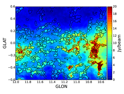
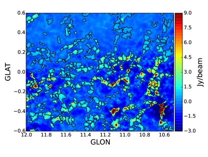
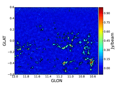
Figure 8: Comparison of molecular cloud clumps identified in the same $\ell=11^{\circ}$ region of Hi-GAL 500 $\mu$m (upper: unfiltered left, high-pass filtered right) and BGPS (lower). Hi-GAL’s higher S/N and absence of atmospheric emission allow for more clumps to be identified than in the ground-based BGPS.

4.1 Clump Densities on the Sky

Table 1 shows the number of clumps in a selection of complete Hi-GAL regions, as well as all of BGPS. Each region is $2^{\circ}\times 2^{\circ}$. Listed are the number of total clumps, the number of clumps with some distance information, and the number of clumps with well-constrained distances. Clumps were considered to have “well-constrained” distances if their DPDFs had a $\text{FW}_{68}\leq 2.3$ kpc. That is, the isoprobability confidence region surrounding the distance of maximum likelihood which contains 68.3% of the total integrated probability has a full width less than 2.3 kpc. This was adopted from Ellsworth-Bowers et al. (2013), which found an empirical cut-off at this point such that clumps with $\text{FW}_{68}\leq 2.3$ kpc either had 78% of the total integrated probability within the most likely kinematic peak, or were located at the tangent distance. Clumps with kinematic distances, regardless of whether the posterior DPDF met the well-constrained criteria, are considered to have some distance information. GRS observations are not available in $\ell=11^{\circ},202^{\circ},\text{or }217^{\circ}$, but there are directed observations of dense gas tracers in $\ell=11^{\circ}$. There is a slight tendency towards more clumps being identified in regions with lower levels of confusion, such as those in the outer galaxy.

Table 1: Distance Statistics

Region	Total	Some distance	Well-constrained
	clumps	information	distance
$\ell=11^{\circ}$	875	96	40
$\ell=30^{\circ}$	979	588	320
$\ell=41^{\circ}$	1027	567	243
$\ell=50^{\circ}$	923	582	392
$\ell=202^{\circ}$	1346	0	0
$\ell=217^{\circ}$	1048	0	0
sum	6198	1833	995
BGPS	8594	3508	1710

Properties of clumps individually could only be compared where clumps identified in each survey aligned with one another. Therefore the overlapping subsections of each map pair were studied for such clumps. Table 2 compares the number of clumps found in these overlapping Hi-GAL and BGPS subregions. Listed are the number of total clumps, the number of clumps with some distance information, and the number of clumps with well-constrained distances. The reduction in number of Hi-GAL clumps in Table 2 as compared to Table 1 is primarily due to the smaller Galactic latitude range covered by BGPS as compared to Hi-GAL. Note that the regions are not consistently sized, and thus comparing numbers between regions is not a useful exercise. Information on the individual clumps being compared is listed in the Appendix.

Table 2: Distance Statistics: Overlapping Subregions

Region	Area	Survey	Total	Some distance	Well-constrained
	(deg2)		clumps	information	distance
$\ell=11^{\circ}$	1.80	Hi-GAL	376	53	30
		BGPS	190	57	34
$\ell=30^{\circ}$	1.44	Hi-GAL	394	234	95
		BGPS	238	187	73
$\ell=41^{\circ}$	2.64	Hi-GAL	650	383	107
		BGPS	63	55	20
$\ell=50^{\circ}$	2.64	Hi-GAL	575	385	232
		BGPS	57	48	33
$\ell=202^{\circ}$	0.85	Hi-GAL	171	0	0
		BGPS	10	0	0
$\ell=217^{\circ}$	1.89	Hi-GAL	323	0	0
		BGPS	15	0	0

In the $\ell=11^{\circ}$ region, the numbers would indicate more clumps with distance information in BGPS than Hi-GAL. However, upon examination of the maps, it is apparent that this is only due to 5 single Hi-GAL clumps being split into two BGPS clumps each, and one single BGPS clump being split into two Hi-GAL clumps. Thus the numbers of clumps with distance information are equal in this region. There are no additional clumps with distance information in Hi-GAL for this region due to it not being covered by GRS. The only velocities are thus from directed observations of dense gas tracers done for BGPS. All additional distances are due to GRS. While the known distances prior, which associates nearby clumps with one another, was used, it did not provide any additional distances in this subset of Hi-GAL observations. The $\ell=202^{\circ}$ and $217^{\circ}$ regions has no distance information due to the lack of GRS observations in the outer Galaxy and a lack of directed observations.

4.2 Angular Sizes

The distributions of deconvolved angular radii is shown in Figure 9 for Hi-GAL (left) and BGPS (right). Rosolowsky et al. (2010) defined the deconvolved radius $\theta_{R}$ of a clump as the geometric mean of the deconvolved major and minor axes of the flux density distribution,

$$\theta_{R}=\eta[(\sigma_{\text{maj}}^{2}-\sigma_{\text{beam}}^{2})(\sigma_{\text{min}}^{2}-\sigma_{\text{beam}}^{2})]^{1/4}.$$ (2)

For Hi-GAL $\sigma_{\text{beam}}=\theta_{\text{FWHM}}/\sqrt{8\ln{2}}=15^{\prime\prime}$, $\theta_{\text{FWHM}}=35^{\prime\prime}$, and $\eta=2.4$ is a factor relating the rms size of the emission distribution to the true size of the source, which is adopted from Rosolowsky et al. (2010). Note that if $\sigma_{\text{min}}<\sigma_{\text{beam}}$ the deconvolved angular radius is non-real. This is the case for 14% of our sources, arising from finite S/N. Mean angular radii for Hi-GAL and BGPS sources are $71\pm 33\arcsec$ and $51\pm 24\arcsec$, respectively. Both follow log-normal distributions (with shape parameters of $\sigma=0.34\pm 0.02$ and $\sigma=0.37\pm 0.01$, respectively), shown in red. We expect that the lognormal distribution is a result of random processes in the observations (such as variations in clump distances and intrinsic sizes), an interpretation which is consistent with the central limit theorem. Thus, Figure 9 is intended to demonstrate the difference in typical sizes found in the two surveys.

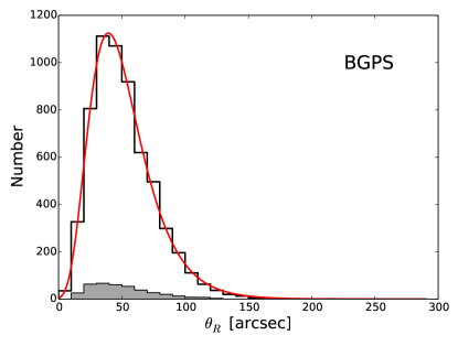
Figure 9: Distributions of deconvolved angular radii with log-normal fits in red. Hi-GAL is shown on the left, including clumps from all of the regions in this substudy, and has a shape parameter of $\sigma=0.34$. BGPS is shown on the right (with all resolved sources included) and has a shape parameter of $\sigma=0.37$. In grey is shown the subsample of BGPS clumps found in regions overlapping our Hi-GAL substudy.

A comparison of the angular radii of clumps matched between Hi-GAL and BGPS is seen in Figure 10. While we do not expect a consistent one-to-one ratio in angular radii, we do expect Hi-GAL clumps to be larger, and this is generally what we see, although less so with those clumps found in the $\ell=30^{\circ}$ region. Dashed lines show a factor of 2 in slope on either side of the identity line and demonstrate the dearth of objects in the lower right of the plot, as compared to the upper left. Clumps can be significantly larger in Hi-GAL due to the dimmer edges of the clumps being above the noise in Hi-GAL, where they were not in BGPS. The $\ell=30^{\circ}$ region contains the edge of the Galactic bar, the bright emission and high confusion levels of which led to the high-pass filter creating more extensive negative bowls. This subtracted more flux than was ideal around the bright Galactic bar, and thus removed flux from the comparatively dim edges of the clumps in this region, to the extent that they were found to be smaller in Hi-GAL than in BGPS. Also of note are the clumps on the left edge of this plot. These are clumps which were unresolved in BGPS, but which we can now resolve with Hi-GAL because Hi-GAL detected faint, extended emission.

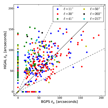
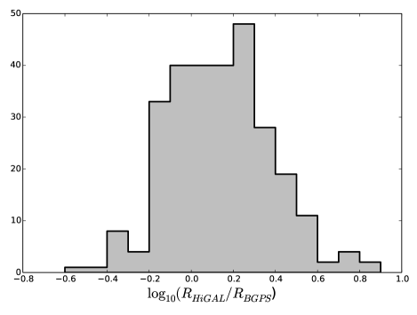
Figure 10: Left: Angular radius in Hi-GAL plotted against angular radius in BGPS, for clumps found in both surveys. Only those clumps which had well constrained distances in both surveys were used for this comparison. Colors correspond to the Hi-GAL region in which the clump was found. Note that in the line of unresolved BGPS clumps on the left of the plot, sources from the $\ell=11^{\circ}$ and $30^{\circ}$ regions are covered by later regions, and not lacking. The solid line is where the radii are equal, while the dashed lines show a factor of two in either direction. Right: Hi-GAL to BGPS radius ratios of matching clumps, excluding those which are unresolved. The mean $\log_{10}(R_{\text{HiGAL}}/R_{\text{BGPS}})$ is 0.14, with a standard deviation of 0.24.

Figure 10 also shows the ratio of radii in the two surveys, for the same objects, but with unresolved objects excluded. The median and mean radius ratios are 1.37 and 1.61, respectively. This agrees with the difference in overall mean radii from the two surveys, as derived from Figure 9.

4.3 Clump Masses

Masses can be calculated for those clumps with well constrained distances using the high-pass filtered flux densities at 500 $\mu$m and the most probable distances from the clumps’ DPDFs. The conversion from flux density to mass is

$$M=\frac{Rd_{\odot}^{2}}{\kappa_{500}B_{500}(T)}S_{500},$$ (3)

where $R=100$ is the gas-to-dust mass ratio, $\kappa=5.04$ cm²g^-1 is the opacity at 500 $\mu$m (Ossenkopf & Henning, 1994), $B_{500}(T)$ is the Planck function at 500 $\mu$m, $d_{\odot}$ is the heliocentric distance, and $S_{500}$ is the integrated flux density. Battersby et al. (2011) used pixel-by-pixel modified blackbody fits of Hi-GAL data to determine that mid-infrared-dark molecular cloud clumps generally span the temperature range 15 K $\lesssim T\lesssim$ 25 K. Furthermore, Dunham et al. (2011) found an NH₃ gas kinetic temperature of $\langle T_{K}\rangle=17.4\pm 5.5$ K for a sample of 199 BGPS sources. For consistency with BGPS, and following these findings, we assume a clump temperature of 20 K.

So as not to limit ourselves to comparing only those clumps which have well constrained distances in both surveys, we calculate mass ratios while holding heliocentric distance constant. Figure 11 shows the ratio of clump masses in Hi-GAL to masses in BGPS, using those clumps listed in the Appendix. Where the ratio is significantly greater than one, the Hi-GAL clumps have much larger angular radii than their BGPS counterparts.

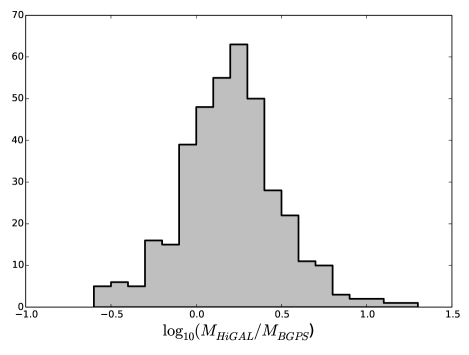
Figure 11: Hi-GAL to BGPS mass ratios of all matching clumps. The mean $\log_{10}(M_{\text{HiGAL}}/M_{\text{BGPS}})$ is 0.20, with a standard deviation of 0.29.

The median mass ratio for the 384 compared clumps is 1.60, and the mean is 2.02. Taken individually, each region had a mean mass ratio within one standard deviation of the other regions. Based on the difference in mean angular radii between the two surveys found in Section 4.2, we would expect this ratio to be 2.7 under the assumption that mass scales as the cube of the angular radius. The observed mass ratio scales as the angular radius squared, suggesting that the clumps are centrally concentrated.

With so few sources available for mass comparison, rather than the precise ratios, the meaningful results are that the median ratio of Hi-GAL mass to BGPS mass is of order unity, and that Hi-GAL masses are generally greater. The same can be said of radii, consistent with greater sensitivity to large-scale structure in Hi-GAL than BGPS, owing both to higher S/N and absence of atmospheric emission in Hi-GAL.

The distribution of masses against physical radii for all resolved Hi-GAL clumps with well-constrained distances is seen in Figure 12. Physical radii are calculated as $R=\theta_{R}d_{\odot}$, where $\theta_{R}$ is angular radius and $d_{\odot}$ is heliocentric distance. Points are colored by heliocentric distance, $d_{\odot}$. If mass scaled as radius cubed, as would happen if the clumps were of constant density, we would see a slope of 3. The figure shows a slope closer to 2 than to 3, thus indicating centrally concentrated masses. (The data are consistent with radial density profiles proportional to $1/R$; however, we caution against concluding a power-law profile in the absence of detailed modeling, including temperature profiles.) Malmquist bias is seen in that the smallest clumps are found at the nearest heliocentric distances, with the largest, most massive objects, being found distant to us.

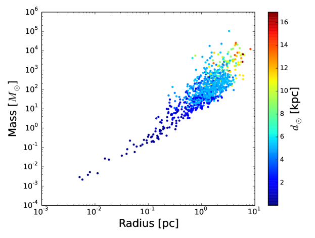
Figure 12: Mass plotted against physical radius for all resolved Hi-GAL sources with well-constrained distances. Colors correspond to heliocentric distance, $d_{\odot}$.

5 Discussion

Compared to BGPS, Hi-GAL detects more sources in all Galactic regions, due to the lack of atmospheric noise. It is especially true in the outer Galaxy, where most sources which are detected with Hi-GAL were lost below the atmospheric noise in BGPS. In BGPS the number of clumps dramatically decreased as observations moved further from the Galactic center. Hi-GAL continues to see sources far from the Galactic center, as well as at Galactic latitudes farther from the the mid-plane.

We identified a relatively constant number of clumps in each region, and, with a mean of 1033 clumps per $2^{\circ}\times 2^{\circ}$ region in our sample, we can expect nearly $2\times 10^{5}$ clumps throughout the entire 360^∘ of Hi-GAL. This is in excellent agreement with Molinari et al. (2016), who found 85,460 clumps in Hi-GAL at 500 $\mu$m between $\ell=-70^{\circ}$ and $\ell=68^{\circ}$. When extrapolated linearly, this predicts $2.2\times 10^{5}$ clumps in the entire Galactic plane. In those regions where GRS is available, 59% of clumps had some distance information, and 33% had well-constrained distances. Thus, in the full $15^{\circ}\leq\ell\leq 56^{\circ}$ range covered by GRS, we can expect approximately 25,000 clumps with some distance information, and 14,000 clumps with well-constrained distances. We will be including other molecular line surveys in addition to GRS: MALT90 (Jackson et al., 2013), ThrUMMs (http://www.astro.ufl.edu/~peterb/research/thrumms/), and SEDIGISM (http://colloques.lam.fr/GESF2014/S3/092_SCHULLE_Frederic.pdf). Once these surveys and the lack of a kinematic distance ambiguity in the outer Galaxy are accounted for, we expect some distance information for 50% of clumps and well-constrained distances for 20% of clumps. This corresponds to 100,000 clumps and 40,000 clumps, respectively, providing a very large sample for investigating Galactic structure and physical properties of molecular cloud clumps.

BGPS used very different techniques for data reduction and large-scale structure removal than what we employed for Hi-GAL. Atmospheric emission was removed directly from the BGPS time-stream. In addition to removing atmospheric emission, this acted as an angular filter, allowing only emission on scales less than about $6\arcmin$ — which roughly corresponded with the array field of view of $7\arcmin.5$ — into the map. An iterative mapping algorithm then restored much of the structure removed in the sky subtraction (Aguirre et al., 2011). Since we had no need to remove atmospheric emission from Hi-GAL, we used a high-pass filter after the maps were made to remove large-scale, smooth dust emission. Despite these very different methods for large-scale structure removal, Hi-GAL and BGPS produce remarkably similar masses. The differences in masses, namely, that Hi-GAL produced generally higher masses, were expected. This is because Hi-GAL can see down to lower flux density levels and therefore can see down to the faint edges of clumps, where often BGPS could only see the brighter central regions.

Of the clumps matched between the two surveys, where the matched were one-to-one and both clumps had well-constrained distances, those distances agreed almost universally within 1 kpc. The one exception was placed at the near distance by BGPS using the HII Region Discovery Survey lookup table prior. In Hi-GAL, this prior was overridden by an EMAF not found by BGPS, which placed the clump at the far distance. Where a single clump in one survey was split in the other survey, distances for each member of the match agreed within 1 kpc, again with one exception. In this case, one Hi-GAL clumps combined two BGPS clumps, one of which had its placement at the tangent distance overridden by an EMAF placing it at the far distance.

The technique used by Molinari et al. (2016) to identify clumps in Hi-GAL was very different from our method. They used the CuTEx algorithm, which first identifies pixels above a curvature threshold. It then simultaneously fits elliptical Gaussian functions and a second-order background surface. Despite the disparate philosophies behind our clump identification techniques, our clump counts are impressively similar. Furthermore, we both see sources at all Galactic latitudes covered by Hi-GAL. Our clumps have slightly larger angular sizes, and once distances for the objects in the Molinari et al. (2016) catalog are determined, we can compare physical properties. That we found such similar results confirms that the objects we are finding are indeed clumps, thus validating both of our results.

The distribution of clumps found in our study of the $\ell=217^{\circ}$ region correspond well visually with what Elia et al. (2013) found in their study of the same Hi-GAL region. The brighter filaments match up particularly well, and although we find more faint clumps, this is understandable, since their study was concerned only with objects for which there was a CO(1–0) velocity measurement. Although we do not yet have distances — and therefore masses and physical radii — for clumps in this outer Galaxy region, it can be noted that the masses and radii for our inner Galaxy clumps span a broader range than those of Elia et al. (2013). We find clumps down to smaller masses, as well as up to greater masses, and similarly for physical radii.

In future work we will extend beyond our sample of six regions and identify clumps in the entirety of Hi-GAL. We will also incorporate other molecular line surveys for the purpose of obtaining kinematic distances for clumps in areas of the Galactic plane not covered by GRS. Furthermore, we will develop two additional priors. The first relies on molecular cloud clumps’ absorption of starlight at short wavelengths and uses that to determine near-infrared extinction (NIREX) distances (Marshall et al., 2009). The second, H I self-absorption (HISA) and H I emission / absorption (HIE/A) techniques, was introduced by Roman-Duval et al. (2009) and Anderson & Bania (2009), and used on ATLASGAL clumps by Wienen et al. (2015).

6 Conclusions

We have made a pilot study with Hi-GAL, comparing dense molecular gas clumps in the Hi-GAL and BGPS surveys. When clumps found in both surveys are compared, derived distances agree within 1 kpc and masses are of order unity, with the mean Hi-GAL to BGPS mass ratio being 1.91. This serves as an external validation for BGPS and instills confidence as we move forward to cataloging the clumps from the entirety of Hi-GAL.

In addition to the sources which were in common with BGPS, Hi-GAL found many additional sources, primarily due to the lack of atmospheric noise. This is especially the case in the outer Galaxy. Being confusion limited, as opposed to atmospheric noise limited, means that we are able to detect clumps to lower flux densities in the outer Galaxy. Whereas BGPS produced a catalog of 8,594 clumps, 20% of which which have well-constrained distances, we expect Hi-GAL to yield $2\times 10^{5}$ clumps, again with 20% having well-constrained distances.

Table A1 lists the clumps matched between Hi-GAL and BGPS. Included are Galactic longitude and latitude ($\ell,b$), integrated flux density ($S$, with subscripts denoting wavelength in $\mu$m), angular radius ($\theta_{R}$), and heliocentric distance ($d_{\odot}$). Due to high-pass filtering, Hi-GAL integrated flux densities and angular radii are attenuated by $(20\pm 10)\%$ and $(4\pm 3)\%$, respectively, as seen in Figure 2. When a clump in one survey has multiple counterparts in the other survey, the additional counterparts are listed on the following lines.

Table A1: Compared Clumps

Hi-GAL					BGPS
$\ell$	$b$	$S_{500}$	$\theta_{R}$	$d_{\odot}$	Catalog #	$\ell$	$b$	$S_{1100}$	$\theta_{R}$	$d_{\odot}$
∘	(∘)	(Jy)	($\arcsec$)	(kpc)		(∘)	(∘)	(Jy)	($\arcsec$)	(kpc)
11.32	-0.53	$22.58\pm 0.19$	95.2	$3.44^{+0.5}_{-0.7}$	2545	11.33	-0.53	$0.37\pm 0.12$	$\cdots$	$3.50^{+0.6}_{-0.8}$
11.09	-0.53	$142.56\pm 0.30$	145.9	$3.30^{+0.4}_{-0.5}$	2508	11.06	-0.49	$0.20\pm 0.08$	$\cdots$	$\cdots$
$\cdots$	$\cdots$	$\cdots$	$\cdots$	$\cdots$	2509	11.06	-0.54	$0.15\pm 0.07$	$\cdots$	$\cdots$
$\cdots$	$\cdots$	$\cdots$	$\cdots$	$\cdots$	2511	11.08	-0.54	$3.56\pm 0.32$	59.4	$2.98^{+0.6}_{-0.7}$
$\cdots$	$\cdots$	$\cdots$	$\cdots$	$\cdots$	2512	11.08	-0.49	$0.38\pm 0.11$	$\cdots$	$\cdots$
$\cdots$	$\cdots$	$\cdots$	$\cdots$	$\cdots$	2514	11.09	-0.50	$0.45\pm 0.14$	37.9	$\cdots$
$\cdots$	$\cdots$	$\cdots$	$\cdots$	$\cdots$	2515	11.10	-0.52	$0.17\pm 0.09$	$\cdots$	$\cdots$
$\cdots$	$\cdots$	$\cdots$	$\cdots$	$\cdots$	2523	11.12	-0.52	$0.23\pm 0.09$	$\cdots$	$\cdots$
10.63	-0.51	$105.37\pm 0.24$	109.0	$\cdots$	2426	10.63	-0.51	$2.89\pm 0.28$	60.3	$\cdots$
10.91	-0.50	$57.76\pm 0.25$	140.4	$\cdots$	2471	10.88	-0.49	$0.54\pm 0.13$	39.9	$\cdots$
$\cdots$	$\cdots$	$\cdots$	$\cdots$	$\cdots$	2473	10.91	-0.49	$0.84\pm 0.16$	39.5	$\cdots$
10.86	-0.49	$20.20\pm 0.15$	75.3	$\cdots$	2468	10.87	-0.49	$0.28\pm 0.11$	18.9	$\cdots$
11.69	-0.48	$67.39\pm 0.25$	131.1	$\cdots$	2570	11.68	-0.47	$1.02\pm 0.19$	50.0	$\cdots$
$\cdots$	$\cdots$	$\cdots$	$\cdots$	$\cdots$	2571	11.70	-0.48	$0.32\pm 0.10$	$\cdots$	$\cdots$
$\cdots$	$\cdots$	$\cdots$	$\cdots$	$\cdots$	2573	11.71	-0.48	$0.12\pm 0.07$	$\cdots$	$\cdots$
11.91	-0.46	$29.88\pm 0.21$	117.0	$\cdots$	2589	11.91	-0.46	$0.66\pm 0.16$	58.5	$\cdots$
11.28	-0.46	$21.71\pm 0.18$	85.8	$3.16^{+0.6}_{-0.7}$	2540	11.28	-0.45	$0.76\pm 0.15$	49.5	$3.20^{+0.6}_{-0.7}$
10.62	-0.44	$70.88\pm 0.16$	64.9	$4.96^{+0.5}_{-0.4}$	2421	10.62	-0.44	$3.61\pm 0.28$	63.2	$4.96^{+0.5}_{-0.4}$
10.84	-0.43	$9.15\pm 0.10$	44.5	$\cdots$	2464	10.84	-0.43	$0.27\pm 0.09$	$\cdots$	$\cdots$
10.60	-0.42	$11.60\pm 0.09$	$\cdots$	$\cdots$	2419	10.60	-0.42	$1.72\pm 0.18$	51.1	$\cdots$
11.77	-0.42	$29.34\pm 0.18$	88.2	$\cdots$	2579	11.76	-0.42	$0.38\pm 0.10$	17.4	$\cdots$
10.83	-0.41	$9.26\pm 0.10$	47.8	$\cdots$	2463	10.84	-0.40	$0.19\pm 0.07$	$\cdots$	$\cdots$
11.11	-0.40	$302.15\pm 0.24$	95.2	$\cdots$	2520	11.11	-0.40	$14.90\pm 0.95$	98.8	$\cdots$
$\cdots$	$\cdots$	$\cdots$	$\cdots$	$\cdots$	2524	11.14	-0.40	$0.49\pm 0.11$	24.6	$\cdots$
10.82	-0.40	$15.01\pm 0.13$	66.1	$\cdots$	2458	10.81	-0.40	$0.80\pm 0.14$	44.3	$\cdots$
$\cdots$	$\cdots$	$\cdots$	$\cdots$	$\cdots$	2460	10.83	-0.40	$0.55\pm 0.14$	40.0	$\cdots$
11.60	-0.38	$43.64\pm 0.22$	115.5	$\cdots$	2563	11.59	-0.39	$1.15\pm 0.18$	66.9	$\cdots$
$\cdots$	$\cdots$	$\cdots$	$\cdots$	$\cdots$	2566	11.62	-0.38	$0.26\pm 0.09$	18.9	$\cdots$
11.07	-0.38	$65.75\pm 0.15$	67.8	$\cdots$	2510	11.07	-0.38	$4.63\pm 0.36$	81.9	$\cdots$
10.62	-0.38	$756.01\pm 0.19$	58.9	$4.96^{+0.5}_{-0.4}$	2418	10.60	-0.37	$3.11\pm 0.23$	52.7	$4.96^{+0.5}_{-0.4}$
$\cdots$	$\cdots$	$\cdots$	$\cdots$	$\cdots$	2424	10.62	-0.39	$42.63\pm 2.61$	80.5	$4.96^{+0.5}_{-0.4}$
10.80	-0.38	$10.44\pm 0.11$	44.3	$\cdots$	2457	10.80	-0.38	$0.64\pm 0.15$	43.8	$\cdots$
$\cdots$	$\cdots$	$\cdots$	$\cdots$	$\cdots$	2459	10.82	-0.39	$0.11\pm 0.07$	$\cdots$	$\cdots$
11.37	-0.38	$17.61\pm 0.17$	86.0	$\cdots$	2546	11.37	-0.38	$0.21\pm 0.08$	$\cdots$	$\cdots$
10.99	-0.37	$71.35\pm 0.20$	95.0	$\cdots$	2484	10.96	-0.36	$0.69\pm 0.12$	39.6	$\cdots$
$\cdots$	$\cdots$	$\cdots$	$\cdots$	$\cdots$	2487	10.98	-0.37	$1.68\pm 0.18$	50.8	$\cdots$
$\cdots$	$\cdots$	$\cdots$	$\cdots$	$\cdots$	2492	11.00	-0.37	$1.25\pm 0.16$	45.2	$\cdots$
$\cdots$	$\cdots$	$\cdots$	$\cdots$	$\cdots$	2494	11.01	-0.39	$0.54\pm 0.12$	30.1	$\cdots$
9.95	-0.37	$44.79\pm 0.15$	71.3	$13.62^{+0.8}_{-0.6}$	2863	13.28	-0.39	$0.25\pm 0.10$	$\cdots$	$\cdots$
10.91	-0.36	$14.34\pm 0.10$	45.6	$\cdots$	2477	10.92	-0.35	$0.70\pm 0.14$	50.6	$\cdots$
10.93	-0.34	$32.99\pm 0.18$	99.7	$\cdots$	$\cdots$	$\cdots$	$\cdots$	$\cdots$	$\cdots$	$\cdots$
11.54	-0.37	$20.70\pm 0.17$	90.7	$\cdots$	2558	11.53	-0.35	$0.23\pm 0.09$	$\cdots$	$\cdots$
$\cdots$	$\cdots$	$\cdots$	$\cdots$	$\cdots$	2559	11.54	-0.37	$0.08\pm 0.06$	$\cdots$	$\cdots$
11.98	-0.35	$10.52\pm 0.12$	47.2	$\cdots$	2601	11.98	-0.35	$0.53\pm 0.12$	15.7	$4.14^{+0.5}_{-0.6}$
11.28	-0.35	$6.41\pm 0.10$	34.5	$\cdots$	2541	11.28	-0.35	$0.20\pm 0.07$	$\cdots$	$\cdots$
10.58	-0.35	$15.26\pm 0.09$	$\cdots$	$4.96^{+0.5}_{-0.4}$	2416	10.58	-0.35	$1.57\pm 0.18$	52.8	$4.96^{+0.5}_{-0.4}$
11.40	-0.33	$26.77\pm 0.21$	117.5	$\cdots$	2549	11.40	-0.34	$0.32\pm 0.11$	42.2	$\cdots$
10.62	-0.34	$177.96\pm 0.16$	59.9	$4.96^{+0.5}_{-0.4}$	2417	10.58	-0.29	$0.36\pm 0.09$	21.6	$\cdots$
10.59	-0.30	$7.31\pm 0.10$	33.0	$\cdots$	$\cdots$	$\cdots$	$\cdots$	$\cdots$	$\cdots$	$\cdots$
$\cdots$	$\cdots$	$\cdots$	$\cdots$	$\cdots$	2425	10.62	-0.33	$11.98\pm 0.79$	105.2	$4.96^{+0.5}_{-0.4}$
10.72	-0.33	$54.35\pm 0.13$	46.8	$4.96^{+0.5}_{-0.4}$	2445	10.72	-0.33	$3.33\pm 0.28$	58.7	$4.96^{+0.5}_{-0.4}$
11.22	-0.32	$9.54\pm 0.13$	58.5	$\cdots$	2536	11.23	-0.32	$0.60\pm 0.14$	51.0	$\cdots$
11.25	-0.32	$14.23\pm 0.14$	60.9	$\cdots$	$\cdots$	$\cdots$	$\cdots$	$\cdots$	$\cdots$	$\cdots$
12.16	-0.32	$12.08\pm 0.16$	83.8	$\cdots$	2620	12.16	-0.32	$0.67\pm 0.15$	56.9	$\cdots$
11.52	-0.33	$40.83\pm 0.21$	107.6	$4.36^{+0.4}_{-0.5}$	2554	11.51	-0.34	$0.24\pm 0.09$	$\cdots$	$\cdots$
$\cdots$	$\cdots$	$\cdots$	$\cdots$	$\cdots$	2556	11.52	-0.32	$0.87\pm 0.16$	63.3	$4.22^{+0.4}_{-0.5}$
10.69	-0.31	$31.58\pm 0.14$	59.8	$4.96^{+0.5}_{-0.4}$	2437	10.69	-0.31	$2.46\pm 0.26$	71.7	$4.96^{+0.5}_{-0.4}$
10.76	-0.31	$22.27\pm 0.16$	81.5	$\cdots$	2455	10.76	-0.30	$0.33\pm 0.11$	26.1	$\cdots$
11.70	-0.30	$14.77\pm 0.14$	62.6	$\cdots$	2572	11.70	-0.30	$0.65\pm 0.16$	50.2	$\cdots$
12.12	-0.29	$17.33\pm 0.15$	84.5	$\cdots$	2616	12.11	-0.30	$0.61\pm 0.14$	27.5	$\cdots$
10.74	-0.30	$10.86\pm 0.11$	42.6	$\cdots$	2448	10.74	-0.30	$0.41\pm 0.12$	36.5	$\cdots$
11.99	-0.27	$66.45\pm 0.22$	111.9	$\cdots$	2602	11.99	-0.29	$0.22\pm 0.08$	$\cdots$	$\cdots$
$\cdots$	$\cdots$	$\cdots$	$\cdots$	$\cdots$	2603	11.99	-0.27	$1.76\pm 0.23$	57.2	$\cdots$
$\cdots$	$\cdots$	$\cdots$	$\cdots$	$\cdots$	2605	12.02	-0.28	$0.26\pm 0.09$	18.0	$\cdots$
12.06	-0.26	$6.61\pm 0.08$	$\cdots$	$\cdots$	2608	12.06	-0.26	$0.48\pm 0.12$	22.1	$\cdots$
12.02	-0.26	$23.15\pm 0.13$	55.3	$\cdots$	2604	12.02	-0.26	$0.67\pm 0.14$	29.1	$\cdots$
11.94	-0.26	$35.74\pm 0.18$	69.4	$\cdots$	2594	11.94	-0.26	$1.26\pm 0.17$	25.9	$\cdots$
11.74	-0.24	$8.28\pm 0.12$	45.9	$\cdots$	2577	11.74	-0.24	$0.19\pm 0.08$	$\cdots$	$\cdots$
10.69	-0.24	$3.15\pm 0.08$	$\cdots$	$\cdots$	2438	10.69	-0.24	$0.14\pm 0.08$	$\cdots$	$\cdots$
$\cdots$	$\cdots$	$\cdots$	$\cdots$	$\cdots$	2439	10.69	-0.25	$0.14\pm 0.07$	$\cdots$	$\cdots$
11.90	-0.22	$25.79\pm 0.18$	83.6	$\cdots$	2587	11.89	-0.22	$1.34\pm 0.17$	46.7	$\cdots$
10.67	-0.22	$45.02\pm 0.14$	49.3	$\cdots$	2434	10.67	-0.22	$2.81\pm 0.25$	62.8	$\cdots$
12.02	-0.21	$38.55\pm 0.18$	72.7	$\cdots$	2606	12.02	-0.21	$1.60\pm 0.19$	49.8	$\cdots$
11.66	-0.20	$10.06\pm 0.14$	75.4	$\cdots$	2569	11.66	-0.19	$0.24\pm 0.09$	16.1	$\cdots$
10.67	-0.20	$35.15\pm 0.13$	58.0	$\cdots$	2433	10.67	-0.20	$1.95\pm 0.21$	57.0	$\cdots$
11.50	-0.19	$8.77\pm 0.12$	52.5	$\cdots$	2553	11.50	-0.20	$0.21\pm 0.08$	$\cdots$	$\cdots$
11.86	-0.19	$10.93\pm 0.12$	44.3	$\cdots$	2586	11.86	-0.19	$0.40\pm 0.11$	$\cdots$	$\cdots$
12.08	-0.18	$38.19\pm 0.22$	120.2	$\cdots$	2609	12.07	-0.20	$0.51\pm 0.13$	38.7	$\cdots$
$\cdots$	$\cdots$	$\cdots$	$\cdots$	$\cdots$	2610	12.08	-0.18	$0.51\pm 0.14$	51.7	$\cdots$
$\cdots$	$\cdots$	$\cdots$	$\cdots$	$\cdots$	2613	12.10	-0.20	$0.45\pm 0.12$	36.8	$\cdots$
11.00	-0.17	$18.21\pm 0.12$	59.4	$\cdots$	2491	11.00	-0.17	$1.47\pm 0.18$	61.8	$\cdots$
10.67	-0.16	$20.74\pm 0.12$	52.1	$3.22^{+0.5}_{-0.6}$	2432	10.67	-0.17	$1.04\pm 0.17$	45.5	$3.20^{+0.6}_{-0.8}$
11.94	-0.15	$51.08\pm 0.12$	41.1	$\cdots$	2592	11.94	-0.15	$2.73\pm 0.25$	44.4	$\cdots$
11.75	-0.14	$50.71\pm 0.14$	55.1	$\cdots$	2576	11.75	-0.14	$1.31\pm 0.17$	43.9	$\cdots$
$\cdots$	$\cdots$	$\cdots$	$\cdots$	$\cdots$	2578	11.76	-0.15	$1.34\pm 0.15$	31.6	$\cdots$
10.98	-0.15	$14.94\pm 0.13$	64.5	$\cdots$	2488	10.98	-0.15	$0.73\pm 0.15$	50.0	$\cdots$
11.47	-0.14	$27.49\pm 0.19$	86.6	$\cdots$	2550	11.46	-0.14	$0.90\pm 0.16$	53.5	$\cdots$
11.90	-0.14	$142.13\pm 0.18$	66.0	$13.70^{+0.4}_{-0.7}$	2590	11.90	-0.14	$6.46\pm 0.45$	65.7	$\cdots$
12.15	-0.14	$3.09\pm 0.07$	$\cdots$	$\cdots$	2619	12.15	-0.14	$0.60\pm 0.13$	40.6	$\cdots$
11.60	-0.13	$20.55\pm 0.14$	57.3	$\cdots$	2565	11.60	-0.13	$0.87\pm 0.14$	41.8	$\cdots$
11.79	-0.14	$21.15\pm 0.19$	98.7	$\cdots$	2582	11.80	-0.13	$0.58\pm 0.13$	39.8	$\cdots$
11.01	-0.13	$2.74\pm 0.08$	25.1	$\cdots$	2493	11.01	-0.13	$0.39\pm 0.11$	32.4	$\cdots$
12.11	-0.13	$16.73\pm 0.09$	$\cdots$	$\cdots$	2615	12.11	-0.13	$0.83\pm 0.12$	10.8	$\cdots$
11.13	-0.13	$57.02\pm 0.14$	66.1	$2.86^{+0.6}_{-0.6}$	2519	11.12	-0.12	$8.56\pm 0.59$	108.9	$3.02^{+0.6}_{-0.7}$
11.11	-0.12	$75.43\pm 0.16$	73.4	$3.28^{+0.5}_{-0.7}$	$\cdots$	$\cdots$	$\cdots$	$\cdots$	$\cdots$	$\cdots$
11.98	-0.13	$20.10\pm 0.15$	66.2	$12.08^{+0.4}_{-0.4}$	2599	11.97	-0.12	$0.76\pm 0.15$	47.3	$12.10^{+0.4}_{-0.4}$
$\cdots$	$\cdots$	$\cdots$	$\cdots$	$\cdots$	2600	11.99	-0.13	$0.51\pm 0.11$	22.8	$12.12^{+0.4}_{-0.3}$
10.68	-0.13	$39.80\pm 0.12$	60.1	$3.04^{+0.6}_{-0.6}$	2436	10.68	-0.12	$1.62\pm 0.18$	54.4	$3.22^{+0.6}_{-0.7}$
10.65	-0.12	$32.68\pm 0.16$	77.7	$3.02^{+0.8}_{-1.1}$	2427	10.65	-0.12	$1.46\pm 0.20$	69.9	$3.10^{+0.9}_{-1.3}$
12.20	-0.12	$221.80\pm 0.19$	81.9	$\cdots$	2623	12.20	-0.12	$7.82\pm 0.51$	63.2	$\cdots$
$\cdots$	$\cdots$	$\cdots$	$\cdots$	$\cdots$	2625	12.21	-0.12	$5.36\pm 0.37$	53.1	$\cdots$
$\cdots$	$\cdots$	$\cdots$	$\cdots$	$\cdots$	2627	12.22	-0.16	$0.23\pm 0.09$	8.6	$\cdots$
11.93	-0.11	$7.90\pm 0.10$	21.1	$\cdots$	2591	11.93	-0.11	$0.33\pm 0.10$	$\cdots$	$\cdots$
11.56	-0.11	$18.25\pm 0.16$	75.8	$\cdots$	2562	11.56	-0.11	$0.12\pm 0.06$	$\cdots$	$\cdots$
11.86	-0.11	$5.40\pm 0.07$	$\cdots$	$\cdots$	2585	11.86	-0.10	$0.36\pm 0.09$	$\cdots$	$\cdots$
12.21	-0.10	$215.54\pm 0.13$	40.9	$\cdots$	2624	12.21	-0.10	$12.88\pm 0.82$	53.5	$\cdots$
11.97	-0.09	$9.21\pm 0.10$	45.8	$\cdots$	2598	11.97	-0.09	$0.63\pm 0.14$	51.1	$\cdots$
11.90	-0.10	$22.42\pm 0.13$	38.6	$\cdots$	2588	11.90	-0.11	$0.85\pm 0.15$	$\cdots$	$\cdots$
11.84	-0.10	$22.45\pm 0.13$	46.9	$\cdots$	2584	11.84	-0.10	$0.95\pm 0.14$	27.9	$\cdots$
10.82	-0.10	$5.29\pm 0.06$	$\cdots$	$\cdots$	2461	10.82	-0.10	$0.24\pm 0.08$	$\cdots$	$\cdots$
10.70	-0.11	$74.00\pm 0.19$	109.9	$\cdots$	2443	10.70	-0.10	$2.05\pm 0.22$	74.5	$\cdots$
$\cdots$	$\cdots$	$\cdots$	$\cdots$	$\cdots$	2447	10.71	-0.12	$0.30\pm 0.07$	$\cdots$	$\cdots$
11.94	-0.10	$11.11\pm 0.11$	45.9	$\cdots$	2593	11.94	-0.10	$0.29\pm 0.09$	$\cdots$	$\cdots$
11.06	-0.10	$63.86\pm 0.20$	104.7	$2.92^{+0.6}_{-0.7}$	2507	11.06	-0.09	$4.69\pm 0.37$	96.2	$3.00^{+0.6}_{-0.7}$
11.20	-0.10	$71.16\pm 0.21$	110.8	$3.22^{+0.5}_{-0.6}$	2530	11.19	-0.10	$3.02\pm 0.29$	78.3	$3.18^{+0.6}_{-0.7}$
$\cdots$	$\cdots$	$\cdots$	$\cdots$	$\cdots$	2531	11.22	-0.10	$0.96\pm 0.14$	10.7	$3.18^{+0.6}_{-0.7}$
10.98	-0.08	$158.98\pm 0.28$	136.4	$3.24^{+0.5}_{-0.6}$	2485	10.97	-0.09	$3.16\pm 0.28$	70.1	$3.58^{+0.5}_{-0.6}$
$\cdots$	$\cdots$	$\cdots$	$\cdots$	$\cdots$	2486	10.98	-0.05	$0.20\pm 0.08$	$\cdots$	$\cdots$
$\cdots$	$\cdots$	$\cdots$	$\cdots$	$\cdots$	2489	11.00	-0.08	$5.71\pm 0.41$	82.1	$2.92^{+0.6}_{-0.7}$
11.77	-0.07	$30.30\pm 0.14$	56.1	$\cdots$	2581	11.77	-0.07	$1.01\pm 0.14$	35.1	$\cdots$
10.81	-0.08	$6.79\pm 0.11$	44.6	$\cdots$	2456	10.79	-0.09	$0.25\pm 0.09$	$\cdots$	$\cdots$
11.17	-0.07	$7.24\pm 0.08$	$\cdots$	$\cdots$	2527	11.17	-0.07	$0.38\pm 0.10$	12.3	$\cdots$
10.72	-0.07	$15.34\pm 0.13$	67.3	$\cdots$	2446	10.72	-0.06	$0.84\pm 0.16$	58.6	$\cdots$
11.72	-0.07	$40.58\pm 0.18$	83.2	$\cdots$	2574	11.72	-0.09	$0.15\pm 0.07$	$\cdots$	$\cdots$
$\cdots$	$\cdots$	$\cdots$	$\cdots$	$\cdots$	2575	11.72	-0.07	$1.80\pm 0.23$	74.0	$\cdots$
11.63	-0.06	$2.58\pm 0.07$	$\cdots$	$\cdots$	2567	11.63	-0.06	$0.26\pm 0.09$	$\cdots$	$\cdots$
11.23	-0.07	$14.84\pm 0.12$	57.6	$3.24^{+0.6}_{-0.7}$	2533	11.23	-0.06	$0.76\pm 0.14$	28.2	$3.24^{+0.6}_{-0.8}$
11.82	-0.06	$13.21\pm 0.14$	53.7	$\cdots$	2583	11.82	-0.06	$0.52\pm 0.13$	44.5	$\cdots$
10.88	-0.05	$5.28\pm 0.08$	$\cdots$	$\cdots$	2469	10.88	-0.05	$0.53\pm 0.11$	36.4	$\cdots$
12.16	-0.04	$0.86\pm 0.04$	$\cdots$	$\cdots$	2621	12.16	-0.04	$0.21\pm 0.08$	$\cdots$	$\cdots$
11.76	-0.04	$14.15\pm 0.13$	52.7	$\cdots$	2580	11.77	-0.04	$0.60\pm 0.12$	24.4	$\cdots$
11.05	-0.04	$5.71\pm 0.09$	$\cdots$	$3.20^{+0.6}_{-0.8}$	2504	11.05	-0.04	$0.47\pm 0.11$	18.8	$3.16^{+0.6}_{-0.8}$
10.86	-0.04	$5.23\pm 0.10$	43.0	$\cdots$	2462	10.82	-0.02	$4.66\pm 0.40$	116.7	$\cdots$
10.82	-0.02	$78.09\pm 0.23$	107.5	$\cdots$	$\cdots$	$\cdots$	$\cdots$	$\cdots$	$\cdots$	$\cdots$
$\cdots$	$\cdots$	$\cdots$	$\cdots$	$\cdots$	2466	10.85	-0.05	$0.09\pm 0.06$	$\cdots$	$\cdots$
12.20	-0.03	$58.95\pm 0.16$	52.4	$\cdots$	2622	12.20	-0.03	$3.56\pm 0.32$	72.8	$\cdots$
12.12	-0.03	$11.59\pm 0.12$	43.4	$\cdots$	2617	12.12	-0.03	$0.65\pm 0.12$	30.7	$\cdots$
11.94	-0.04	$52.62\pm 0.17$	86.3	$\cdots$	2595	11.94	-0.04	$4.02\pm 0.34$	82.0	$\cdots$
12.03	-0.03	$36.93\pm 0.18$	79.0	$9.66^{+0.8}_{-0.7}$	2607	12.03	-0.03	$1.42\pm 0.19$	49.2	$9.66^{+0.8}_{-0.7}$
12.15	-0.03	$4.41\pm 0.10$	41.0	$\cdots$	2618	12.15	-0.02	$0.26\pm 0.09$	$\cdots$	$\cdots$
11.03	-0.03	$3.64\pm 0.08$	$\cdots$	$\cdots$	2499	11.03	-0.03	$0.15\pm 0.06$	$\cdots$	$\cdots$
10.68	-0.03	$89.46\pm 0.19$	73.7	$\cdots$	2435	10.68	-0.03	$3.82\pm 0.32$	64.3	$\cdots$
10.62	-0.03	$29.28\pm 0.17$	72.4	$\cdots$	2420	10.62	-0.03	$1.82\pm 0.20$	64.3	$\cdots$
$\cdots$	$\cdots$	$\cdots$	$\cdots$	$\cdots$	2423	10.62	-0.06	$0.27\pm 0.09$	33.4	$\cdots$
10.97	-0.02	$10.25\pm 0.12$	52.0	$\cdots$	2483	10.97	-0.02	$0.35\pm 0.10$	20.9	$\cdots$
10.57	-0.02	$15.29\pm 0.13$	51.8	$\cdots$	2415	10.57	-0.02	$0.50\pm 0.11$	29.6	$\cdots$
11.65	-0.01	$6.50\pm 0.10$	42.0	$\cdots$	2568	11.64	-0.01	$0.19\pm 0.07$	$\cdots$	$\cdots$
12.25	-0.00	$7.99\pm 0.10$	25.1	$\cdots$	2634	12.25	-0.00	$0.65\pm 0.14$	30.1	$\cdots$
11.15	-0.01	$12.12\pm 0.16$	82.7	$\cdots$	2526	11.15	-0.00	$0.39\pm 0.11$	23.9	$\cdots$
11.95	0.00	$1.73\pm 0.07$	$\cdots$	$\cdots$	2597	11.95	-0.00	$0.17\pm 0.08$	$\cdots$	$\cdots$
11.27	0.01	$4.94\pm 0.11$	46.1	$\cdots$	2539	11.26	0.01	$0.42\pm 0.12$	33.8	$\cdots$
11.40	0.03	$29.16\pm 0.19$	103.2	$\cdots$	2547	11.39	0.03	$0.15\pm 0.07$	$\cdots$	$\cdots$
$\cdots$	$\cdots$	$\cdots$	$\cdots$	$\cdots$	2548	11.40	0.02	$0.40\pm 0.11$	$\cdots$	$\cdots$
11.10	0.01	$6.35\pm 0.12$	50.7	$\cdots$	2513	11.09	0.01	$0.38\pm 0.10$	29.7	$\cdots$
$\cdots$	$\cdots$	$\cdots$	$\cdots$	$\cdots$	2516	11.10	0.01	$0.15\pm 0.07$	$\cdots$	$\cdots$
10.75	0.02	$48.56\pm 0.17$	80.7	$\cdots$	2451	10.74	0.04	$0.11\pm 0.06$	$\cdots$	$\cdots$
$\cdots$	$\cdots$	$\cdots$	$\cdots$	$\cdots$	2452	10.74	0.01	$3.35\pm 0.30$	82.8	$\cdots$
10.96	0.02	$74.57\pm 0.15$	50.6	$\cdots$	2481	10.96	0.02	$4.48\pm 0.34$	59.0	$\cdots$
10.70	0.01	$54.17\pm 0.18$	95.2	$\cdots$	2442	10.70	-0.00	$0.42\pm 0.10$	$\cdots$	$\cdots$
$\cdots$	$\cdots$	$\cdots$	$\cdots$	$\cdots$	2444	10.71	0.01	$1.74\pm 0.23$	77.4	$\cdots$
11.03	0.03	$10.40\pm 0.09$	18.1	$\cdots$	2496	11.02	0.03	$0.29\pm 0.08$	$\cdots$	$\cdots$
$\cdots$	$\cdots$	$\cdots$	$\cdots$	$\cdots$	2498	11.03	0.03	$0.62\pm 0.10$	17.8	$\cdots$
12.24	0.04	$5.57\pm 0.10$	35.4	$\cdots$	2628	12.24	0.04	$0.23\pm 0.08$	$\cdots$	$\cdots$
10.69	0.04	$28.37\pm 0.16$	85.0	$\cdots$	2441	10.69	0.05	$0.52\pm 0.13$	37.0	$\cdots$
11.11	0.05	$18.21\pm 0.09$	$\cdots$	$\cdots$	2521	11.11	0.05	$0.81\pm 0.12$	$\cdots$	$\cdots$
11.15	0.05	$6.45\pm 0.10$	38.7	$\cdots$	2525	11.14	0.05	$0.22\pm 0.07$	$\cdots$	$\cdots$
10.93	0.05	$5.42\pm 0.09$	$\cdots$	$\cdots$	2476	10.92	0.05	$0.57\pm 0.12$	35.4	$\cdots$
$\cdots$	$\cdots$	$\cdots$	$\cdots$	$\cdots$	2479	10.94	0.04	$0.23\pm 0.08$	$\cdots$	$\cdots$
11.03	0.06	$40.47\pm 0.13$	37.0	$\cdots$	2500	11.03	0.06	$2.98\pm 0.27$	55.8	$\cdots$
10.85	0.06	$16.60\pm 0.17$	90.8	$\cdots$	2465	10.85	0.06	$0.34\pm 0.10$	26.9	$\cdots$
11.23	0.06	$30.43\pm 0.20$	102.9	$\cdots$	2535	11.24	0.06	$0.45\pm 0.12$	$\cdots$	$\cdots$
11.19	0.07	$18.93\pm 0.16$	80.1	$\cdots$	2528	11.18	0.06	$0.49\pm 0.12$	35.6	$\cdots$
$\cdots$	$\cdots$	$\cdots$	$\cdots$	$\cdots$	2529	11.19	0.07	$0.31\pm 0.10$	$\cdots$	$\cdots$
10.90	0.07	$9.84\pm 0.10$	29.0	$\cdots$	2472	10.90	0.07	$1.46\pm 0.20$	65.3	$\cdots$
11.09	0.07	$18.25\pm 0.13$	46.4	$\cdots$	2517	11.09	0.07	$0.64\pm 0.13$	18.2	$\cdots$
10.93	0.07	$6.78\pm 0.09$	38.7	$\cdots$	2478	10.93	0.07	$0.62\pm 0.13$	43.7	$\cdots$
10.67	0.10	$72.81\pm 0.22$	116.6	$\cdots$	2430	10.67	0.09	$2.70\pm 0.27$	89.9	$2.48^{+0.8}_{-1.2}$
10.92	0.09	$2.67\pm 0.08$	$\cdots$	$\cdots$	2474	10.92	0.09	$0.17\pm 0.07$	$\cdots$	$\cdots$
$\cdots$	$\cdots$	$\cdots$	$\cdots$	$\cdots$	2475	10.92	0.10	$0.09\pm 0.05$	$\cdots$	$\cdots$
11.06	0.10	$6.28\pm 0.09$	23.6	$\cdots$	2505	11.06	0.10	$0.40\pm 0.10$	25.5	$\cdots$
$\cdots$	$\cdots$	$\cdots$	$\cdots$	$\cdots$	2506	11.07	0.09	$0.13\pm 0.06$	$\cdots$	$\cdots$
12.09	0.11	$1.95\pm 0.07$	$\cdots$	$\cdots$	2612	12.09	0.11	$0.25\pm 0.09$	21.5	$\cdots$
11.12	0.12	$19.38\pm 0.16$	73.5	$\cdots$	2522	11.12	0.12	$0.38\pm 0.10$	37.7	$\cdots$
10.86	0.13	$28.11\pm 0.19$	82.4	$\cdots$	2467	10.86	0.13	$1.38\pm 0.19$	46.6	$\cdots$
10.96	0.15	$64.78\pm 0.21$	121.0	$14.08^{+1.0}_{-0.7}$	2482	10.96	0.14	$1.48\pm 0.20$	58.0	$\cdots$
12.21	0.14	$53.89\pm 0.21$	94.9	$3.54^{+0.4}_{-0.5}$	2626	12.22	0.14	$2.65\pm 0.26$	70.6	$3.52^{+0.5}_{-0.5}$
11.22	0.13	$38.45\pm 0.20$	105.1	$\cdots$	2532	11.22	0.11	$0.35\pm 0.10$	18.9	$\cdots$
$\cdots$	$\cdots$	$\cdots$	$\cdots$	$\cdots$	2534	11.22	0.13	$0.79\pm 0.15$	50.7	$\cdots$
11.11	0.14	$10.80\pm 0.12$	42.4	$\cdots$	2518	11.11	0.14	$0.33\pm 0.09$	$\cdots$	$\cdots$
11.04	0.14	$34.76\pm 0.17$	77.7	$\cdots$	2501	11.03	0.14	$0.42\pm 0.09$	20.6	$\cdots$
$\cdots$	$\cdots$	$\cdots$	$\cdots$	$\cdots$	2502	11.05	0.14	$0.46\pm 0.11$	25.6	$\cdots$
11.00	0.15	$30.20\pm 0.18$	91.5	$\cdots$	2490	10.99	0.14	$0.22\pm 0.08$	$\cdots$	$\cdots$
11.54	0.19	$3.19\pm 0.08$	$\cdots$	$\cdots$	2557	11.53	0.19	$0.24\pm 0.08$	$\cdots$	$\cdots$
11.50	0.21	$27.87\pm 0.18$	86.4	$\cdots$	2552	11.49	0.21	$1.26\pm 0.18$	65.0	$\cdots$
$\cdots$	$\cdots$	$\cdots$	$\cdots$	$\cdots$	2555	11.51	0.20	$0.24\pm 0.08$	28.3	$\cdots$
11.27	0.22	$16.92\pm 0.17$	84.8	$\cdots$	2537	11.27	0.22	$0.49\pm 0.13$	53.1	$\cdots$
12.29	0.24	$24.92\pm 0.21$	115.2	$\cdots$	2639	12.30	0.25	$0.41\pm 0.12$	29.5	$\cdots$
11.60	0.26	$10.38\pm 0.15$	73.5	$3.02^{+0.6}_{-0.7}$	2564	11.60	0.26	$0.23\pm 0.09$	$\cdots$	$3.04^{+0.6}_{-0.7}$
11.55	0.26	$28.43\pm 0.18$	85.1	$3.14^{+0.4}_{-0.5}$	2560	11.53	0.27	$0.74\pm 0.15$	40.1	$3.16^{+0.5}_{-0.6}$
$\cdots$	$\cdots$	$\cdots$	$\cdots$	$\cdots$	2561	11.55	0.26	$0.60\pm 0.12$	34.9	$3.06^{+0.5}_{-0.6}$
11.29	0.32	$6.86\pm 0.12$	43.6	$\cdots$	2542	11.28	0.32	$0.34\pm 0.10$	20.1	$\cdots$
12.24	0.35	$7.41\pm 0.12$	54.9	$\cdots$	2629	12.24	0.34	$0.34\pm 0.10$	22.8	$\cdots$
$\cdots$	$\cdots$	$\cdots$	$\cdots$	$\cdots$	2632	12.24	0.36	$0.10\pm 0.06$	$\cdots$	$\cdots$
12.36	0.51	$3.15\pm 0.08$	27.0	$2.06^{+0.6}_{-0.8}$	2647	12.37	0.51	$0.69\pm 0.14$	42.7	$2.42^{+0.6}_{-0.7}$
11.00	0.56	$28.21\pm 0.31$	203.3	$\cdots$	2495	11.02	0.54	$0.30\pm 0.10$	$\cdots$	$\cdots$
29.90	-0.81	$34.60\pm 0.11$	58.2	$4.58^{+0.3}_{-0.3}$	5075	29.90	-0.80	$1.12\pm 0.30$	41.8	$4.58^{+0.4}_{-0.4}$
29.96	-0.78	$88.38\pm 0.18$	116.5	$4.58^{+0.4}_{-0.4}$	5088	29.95	-0.79	$1.88\pm 0.42$	51.8	$4.58^{+0.4}_{-0.4}$
$\cdots$	$\cdots$	$\cdots$	$\cdots$	$\cdots$	5089	29.96	-0.78	$1.16\pm 0.34$	37.2	$4.62^{+0.4}_{-0.4}$
29.89	-0.78	$94.77\pm 0.20$	117.6	$4.52^{+0.4}_{-0.4}$	5069	29.88	-0.78	$1.43\pm 0.37$	34.9	$4.54^{+0.4}_{-0.4}$
$\cdots$	$\cdots$	$\cdots$	$\cdots$	$\cdots$	5071	29.90	-0.78	$0.75\pm 0.29$	$\cdots$	$4.54^{+0.4}_{-0.4}$
29.60	-0.62	$154.57\pm 0.21$	128.4	$4.24^{+0.5}_{-0.5}$	5028	29.60	-0.61	$5.94\pm 0.57$	83.9	$4.26^{+0.4}_{-0.4}$
$\cdots$	$\cdots$	$\cdots$	$\cdots$	$\cdots$	5030	29.61	-0.58	$0.76\pm 0.18$	45.3	$4.20^{+0.4}_{-0.4}$
30.45	-0.50	$9.66\pm 0.07$	36.5	$\cdots$	5196	30.46	-0.50	$0.74\pm 0.16$	53.1	$\cdots$
30.46	-0.49	$17.59\pm 0.10$	65.0	$\cdots$	$\cdots$	$\cdots$	$\cdots$	$\cdots$	$\cdots$	$\cdots$
29.87	-0.50	$12.58\pm 0.10$	65.3	$3.86^{+0.3}_{-0.3}$	5065	29.86	-0.49	$0.27\pm 0.09$	29.2	$3.90^{+0.3}_{-0.3}$
30.37	-0.48	$5.05\pm 0.08$	52.3	$2.88^{+0.3}_{-0.4}$	5173	30.38	-0.48	$0.48\pm 0.12$	47.8	$2.94^{+0.5}_{-0.5}$
29.88	-0.47	$15.49\pm 0.14$	95.1	$\cdots$	5068	29.88	-0.47	$0.46\pm 0.12$	48.6	$\cdots$
29.84	-0.48	$8.93\pm 0.08$	34.6	$3.80^{+0.3}_{-0.3}$	5062	29.84	-0.48	$0.51\pm 0.10$	22.7	$3.82^{+0.3}_{-0.3}$
30.39	-0.47	$4.29\pm 0.07$	36.6	$\cdots$	5180	30.40	-0.46	$0.24\pm 0.09$	22.9	$2.88^{+0.4}_{-0.4}$
29.64	-0.44	$18.02\pm 0.14$	93.1	$\cdots$	5038	29.65	-0.44	$0.55\pm 0.12$	41.2	$\cdots$
29.47	-0.43	$5.24\pm 0.08$	43.5	$\cdots$	5006	29.47	-0.42	$0.44\pm 0.12$	46.7	$\cdots$
29.98	-0.42	$45.76\pm 0.17$	107.6	$4.06^{+0.4}_{-0.3}$	5091	29.98	-0.42	$1.93\pm 0.24$	81.4	$\cdots$
29.63	-0.38	$10.59\pm 0.11$	73.7	$\cdots$	5036	29.63	-0.38	$0.40\pm 0.10$	38.1	$\cdots$
30.44	-0.38	$10.58\pm 0.07$	$\cdots$	$\cdots$	5191	30.44	-0.38	$0.76\pm 0.13$	26.7	$\cdots$
29.55	-0.36	$14.44\pm 0.12$	77.8	$4.94^{+0.4}_{-0.4}$	5019	29.54	-0.35	$0.23\pm 0.08$	$\cdots$	$\cdots$
$\cdots$	$\cdots$	$\cdots$	$\cdots$	$\cdots$	5020	29.56	-0.36	$0.12\pm 0.06$	$\cdots$	$4.94^{+0.4}_{-0.4}$
30.26	-0.33	$29.34\pm 0.15$	95.6	$\cdots$	5141	30.26	-0.33	$0.85\pm 0.15$	62.0	$\cdots$
$\cdots$	$\cdots$	$\cdots$	$\cdots$	$\cdots$	5142	30.27	-0.31	$0.12\pm 0.06$	$\cdots$	$\cdots$
30.36	-0.33	$18.71\pm 0.12$	65.6	$\cdots$	5165	30.36	-0.36	$0.08\pm 0.05$	$\cdots$	$\cdots$
$\cdots$	$\cdots$	$\cdots$	$\cdots$	$\cdots$	5166	30.36	-0.33	$0.94\pm 0.14$	56.3	$\cdots$
29.91	-0.30	$34.19\pm 0.15$	113.7	$\cdots$	5072	29.90	-0.30	$0.37\pm 0.10$	42.0	$\cdots$
$\cdots$	$\cdots$	$\cdots$	$\cdots$	$\cdots$	5073	29.90	-0.28	$0.24\pm 0.08$	18.9	$\cdots$
$\cdots$	$\cdots$	$\cdots$	$\cdots$	$\cdots$	5077	29.91	-0.33	$0.53\pm 0.13$	44.0	$\cdots$
$\cdots$	$\cdots$	$\cdots$	$\cdots$	$\cdots$	5078	29.92	-0.28	$0.39\pm 0.11$	39.1	$\cdots$
29.76	-0.32	$5.83\pm 0.10$	44.7	$\cdots$	5049	29.77	-0.31	$0.32\pm 0.09$	$\cdots$	$4.98^{+0.4}_{-0.4}$
30.43	-0.30	$17.93\pm 0.10$	57.3	$8.68^{+0.5}_{-0.7}$	5189	30.43	-0.30	$1.21\pm 0.15$	56.8	$8.70^{+0.5}_{-0.7}$
29.97	-0.31	$10.00\pm 0.11$	67.9	$\cdots$	5086	29.96	-0.30	$0.43\pm 0.11$	37.3	$5.00^{+0.4}_{-0.4}$
30.40	-0.30	$22.48\pm 0.10$	50.2	$8.72^{+0.5}_{-0.7}$	5184	30.40	-0.30	$2.06\pm 0.21$	68.2	$8.72^{+0.5}_{-0.7}$
29.93	-0.29	$9.25\pm 0.09$	57.7	$\cdots$	5082	29.93	-0.29	$0.31\pm 0.09$	$\cdots$	$\cdots$
30.31	-0.30	$38.48\pm 0.17$	121.4	$\cdots$	5150	30.30	-0.29	$1.31\pm 0.19$	65.8	$5.34^{+0.6}_{-0.5}$
30.27	-0.29	$15.78\pm 0.10$	60.3	$\cdots$	5137	30.25	-0.29	$0.14\pm 0.07$	13.1	$\cdots$
$\cdots$	$\cdots$	$\cdots$	$\cdots$	$\cdots$	5139	30.27	-0.29	$0.91\pm 0.14$	57.4	$\cdots$
30.09	-0.28	$8.63\pm 0.09$	50.5	$\cdots$	5109	30.09	-0.28	$0.35\pm 0.09$	35.1	$5.20^{+0.4}_{-0.4}$
30.05	-0.28	$8.66\pm 0.08$	40.0	$\cdots$	5105	30.05	-0.28	$0.35\pm 0.10$	26.9	$5.10^{+0.4}_{-0.4}$
30.34	-0.28	$14.14\pm 0.11$	76.2	$\cdots$	5157	30.34	-0.29	$0.15\pm 0.06$	$\cdots$	$\cdots$
$\cdots$	$\cdots$	$\cdots$	$\cdots$	$\cdots$	5164	30.35	-0.27	$0.81\pm 0.14$	52.9	$\cdots$
30.01	-0.27	$173.40\pm 0.22$	118.0	$9.08^{+0.6}_{-0.9}$	5096	30.01	-0.27	$8.46\pm 0.58$	91.5	$5.52^{+0.5}_{-0.5}$
$\cdots$	$\cdots$	$\cdots$	$\cdots$	$\cdots$	5104	30.04	-0.26	$1.09\pm 0.15$	52.9	$\cdots$
29.58	-0.27	$4.20\pm 0.07$	$\cdots$	$\cdots$	5025	29.58	-0.27	$0.54\pm 0.10$	23.0	$\cdots$
29.83	-0.26	$2.15\pm 0.05$	$\cdots$	$5.10^{+0.4}_{-0.3}$	5059	29.83	-0.26	$0.14\pm 0.07$	$\cdots$	$\cdots$
29.78	-0.27	$20.95\pm 0.11$	58.3	$\cdots$	5052	29.78	-0.27	$1.60\pm 0.17$	57.8	$9.06^{+0.3}_{-0.4}$
$\cdots$	$\cdots$	$\cdots$	$\cdots$	$\cdots$	5053	29.78	-0.30	$0.11\pm 0.06$	$\cdots$	$\cdots$
30.10	-0.26	$20.68\pm 0.11$	64.0	$\cdots$	5113	30.11	-0.26	$1.04\pm 0.15$	48.0	$\cdots$
29.76	-0.24	$55.67\pm 0.18$	136.1	$\cdots$	5047	29.75	-0.24	$3.29\pm 0.30$	118.7	$\cdots$
$\cdots$	$\cdots$	$\cdots$	$\cdots$	$\cdots$	5048	29.78	-0.23	$1.55\pm 0.19$	75.7	$\cdots$
29.60	-0.26	$22.60\pm 0.17$	121.4	$\cdots$	5029	29.60	-0.25	$0.70\pm 0.14$	61.1	$\cdots$
29.91	-0.25	$5.85\pm 0.08$	60.9	$\cdots$	5074	29.90	-0.23	$3.80\pm 0.34$	117.2	$5.42^{+0.6}_{-0.5}$
29.89	-0.22	$37.51\pm 0.14$	82.3	$5.46^{+0.6}_{-0.5}$	$\cdots$	$\cdots$	$\cdots$	$\cdots$	$\cdots$	$\cdots$
29.46	-0.25	$26.42\pm 0.16$	110.7	$4.24^{+0.3}_{-0.4}$	5005	29.46	-0.24	$0.31\pm 0.10$	27.6	$4.20^{+0.4}_{-0.4}$
$\cdots$	$\cdots$	$\cdots$	$\cdots$	$\cdots$	5011	29.48	-0.25	$0.40\pm 0.10$	35.4	$4.24^{+0.4}_{-0.4}$
30.43	-0.23	$171.53\pm 0.17$	87.2	$8.56^{+0.5}_{-0.8}$	5187	30.43	-0.23	$13.97\pm 0.91$	117.5	$8.58^{+0.5}_{-0.7}$
29.70	-0.22	$9.20\pm 0.10$	62.8	$\cdots$	5042	29.70	-0.22	$0.40\pm 0.11$	41.4	$\cdots$
29.46	-0.21	$14.31\pm 0.10$	62.5	$\cdots$	5008	29.47	-0.21	$0.40\pm 0.10$	31.7	$\cdots$
30.30	-0.22	$103.83\pm 0.18$	124.5	$\cdots$	5144	30.27	-0.23	$0.73\pm 0.11$	38.5	$7.20^{+1.0}_{-1.0}$
$\cdots$	$\cdots$	$\cdots$	$\cdots$	$\cdots$	5149	30.30	-0.22	$6.21\pm 0.46$	115.3	$\cdots$
29.83	-0.19	$9.30\pm 0.11$	68.4	$4.84^{+0.4}_{-0.4}$	5057	29.83	-0.19	$1.15\pm 0.18$	76.9	$\cdots$
29.68	-0.20	$7.60\pm 0.09$	50.6	$5.06^{+0.4}_{-0.4}$	5040	29.68	-0.20	$0.11\pm 0.06$	$\cdots$	$\cdots$
$\cdots$	$\cdots$	$\cdots$	$\cdots$	$\cdots$	5041	29.68	-0.19	$0.13\pm 0.07$	$\cdots$	$\cdots$
30.22	-0.18	$161.42\pm 0.18$	102.3	$\cdots$	5125	30.22	-0.18	$12.16\pm 0.81$	122.0	$\cdots$
29.49	-0.18	$56.39\pm 0.16$	96.1	$\cdots$	5012	29.49	-0.18	$2.82\pm 0.26$	81.6	$\cdots$
29.44	-0.17	$25.24\pm 0.11$	44.6	$\cdots$	5003	29.44	-0.17	$0.70\pm 0.13$	$\cdots$	$\cdots$
30.00	-0.15	$19.50\pm 0.09$	47.5	$\cdots$	5094	29.99	-0.17	$0.50\pm 0.10$	29.1	$\cdots$
$\cdots$	$\cdots$	$\cdots$	$\cdots$	$\cdots$	5095	30.00	-0.15	$1.23\pm 0.17$	54.9	$\cdots$
30.31	-0.15	$16.95\pm 0.10$	55.7	$6.04^{+1.2}_{-0.6}$	5153	30.32	-0.15	$1.66\pm 0.20$	71.2	$6.06^{+1.3}_{-0.6}$
30.37	-0.14	$14.28\pm 0.07$	35.4	$7.12^{+1.0}_{-1.0}$	5170	30.38	-0.14	$2.78\pm 0.23$	76.1	$7.12^{+1.0}_{-1.0}$
30.07	-0.14	$15.67\pm 0.13$	102.9	$4.94^{+0.5}_{-0.5}$	5107	30.07	-0.14	$0.95\pm 0.15$	74.9	$\cdots$
$\cdots$	$\cdots$	$\cdots$	$\cdots$	$\cdots$	5108	30.08	-0.15	$0.12\pm 0.05$	$\cdots$	$\cdots$
30.20	-0.12	$27.46\pm 0.13$	85.3	$\cdots$	5120	30.17	-0.13	$0.20\pm 0.07$	$\cdots$	$\cdots$
$\cdots$	$\cdots$	$\cdots$	$\cdots$	$\cdots$	5121	30.20	-0.12	$2.71\pm 0.27$	93.3	$\cdots$
30.01	-0.13	$12.81\pm 0.07$	30.3	$5.18^{+0.5}_{-0.5}$	5097	30.01	-0.12	$1.17\pm 0.14$	44.5	$5.24^{+0.5}_{-0.5}$
30.43	-0.11	$43.20\pm 0.12$	70.7	$\cdots$	5190	30.43	-0.11	$4.80\pm 0.36$	99.7	$\cdots$
30.35	-0.12	$55.93\pm 0.14$	90.9	$\cdots$	5160	30.34	-0.12	$5.21\pm 0.39$	103.6	$7.12^{+1.0}_{-1.0}$
30.39	-0.11	$116.72\pm 0.14$	87.0	$\cdots$	5179	30.39	-0.11	$9.42\pm 0.62$	102.6	$7.12^{+1.0}_{-1.0}$
29.66	-0.10	$7.57\pm 0.10$	72.4	$\cdots$	5039	29.67	-0.10	$0.46\pm 0.12$	58.5	$\cdots$
29.84	-0.10	$9.56\pm 0.07$	27.2	$5.56^{+0.5}_{-0.4}$	5061	29.84	-0.10	$1.50\pm 0.18$	68.2	$5.56^{+0.5}_{-0.4}$
29.82	-0.09	$9.22\pm 0.07$	$\cdots$	$5.52^{+0.5}_{-0.4}$	5058	29.82	-0.09	$0.88\pm 0.13$	37.8	$\cdots$
30.21	-0.09	$6.99\pm 0.08$	52.8	$\cdots$	5127	30.21	-0.09	$1.32\pm 0.19$	79.8	$\cdots$
29.47	-0.09	$10.64\pm 0.10$	60.0	$\cdots$	5009	29.47	-0.09	$0.40\pm 0.11$	33.0	$\cdots$
30.14	-0.07	$20.68\pm 0.10$	57.9	$4.66^{+0.5}_{-0.5}$	5116	30.14	-0.07	$1.89\pm 0.22$	68.3	$4.68^{+0.5}_{-0.4}$
$\cdots$	$\cdots$	$\cdots$	$\cdots$	$\cdots$	5117	30.14	-0.04	$0.10\pm 0.06$	$\cdots$	$\cdots$
30.11	-0.07	$10.05\pm 0.09$	49.2	$4.76^{+0.5}_{-0.5}$	5112	30.11	-0.07	$0.90\pm 0.16$	55.0	$\cdots$
29.55	-0.08	$15.58\pm 0.14$	103.1	$\cdots$	5022	29.56	-0.07	$0.48\pm 0.12$	38.9	$\cdots$
29.94	-0.06	$186.72\pm 0.10$	59.4	$5.36^{+0.5}_{-0.4}$	5079	29.92	-0.06	$65.12\pm 3.96$	157.1	$5.44^{+0.5}_{-0.4}$
29.92	-0.05	$283.15\pm 0.14$	85.5	$5.46^{+0.6}_{-0.4}$	$\cdots$	$\cdots$	$\cdots$	$\cdots$	$\cdots$	$\cdots$
30.40	-0.05	$2.28\pm 0.05$	$\cdots$	$6.93^{+0.9}_{-0.9}$	5183	30.40	-0.05	$0.40\pm 0.10$	34.9	$6.12^{+1.1}_{-0.6}$
29.86	-0.05	$83.02\pm 0.10$	43.7	$5.60^{+0.5}_{-0.4}$	5067	29.86	-0.05	$11.67\pm 0.74$	88.8	$5.60^{+0.5}_{-0.4}$
29.42	-0.05	$8.66\pm 0.09$	60.8	$5.10^{+0.5}_{-0.5}$	5002	29.42	-0.05	$0.57\pm 0.16$	40.1	$\cdots$
29.84	-0.04	$15.12\pm 0.08$	31.4	$5.54^{+0.5}_{-0.4}$	5063	29.84	-0.04	$3.69\pm 0.28$	70.2	$5.54^{+0.5}_{-0.4}$
30.45	-0.03	$19.79\pm 0.10$	54.2	$11.40^{+0.4}_{-0.4}$	5192	30.45	-0.03	$2.39\pm 0.26$	85.1	$11.40^{+0.4}_{-0.4}$
29.53	-0.02	$27.42\pm 0.17$	120.3	$\cdots$	5017	29.53	-0.01	$1.06\pm 0.17$	76.4	$\cdots$
30.29	-0.03	$4.27\pm 0.07$	45.1	$\cdots$	5145	30.28	-0.03	$0.24\pm 0.09$	$\cdots$	$\cdots$
$\cdots$	$\cdots$	$\cdots$	$\cdots$	$\cdots$	5147	30.29	-0.02	$0.67\pm 0.14$	52.0	$\cdots$
29.96	-0.02	$304.84\pm 0.13$	60.5	$5.26^{+0.3}_{-0.3}$	5087	29.96	-0.01	$35.71\pm 2.19$	119.3	$5.30^{+0.3}_{-0.3}$
29.94	0.02	$4.88\pm 0.06$	$\cdots$	$5.26^{+0.3}_{-0.3}$	$\cdots$	$\cdots$	$\cdots$	$\cdots$	$\cdots$	$\cdots$
$\cdots$	$\cdots$	$\cdots$	$\cdots$	$\cdots$	5093	29.99	-0.01	$2.08\pm 0.15$	34.3	$\cdots$
29.62	-0.00	$14.56\pm 0.13$	88.0	$\cdots$	5032	29.62	-0.00	$0.80\pm 0.16$	72.6	$\cdots$
30.42	-0.01	$5.38\pm 0.08$	51.3	$\cdots$	5186	30.42	-0.00	$0.56\pm 0.13$	48.4	$\cdots$
30.38	-0.01	$6.37\pm 0.06$	16.2	$\cdots$	5175	30.38	-0.00	$0.43\pm 0.09$	23.8	$\cdots$
29.89	-0.01	$56.18\pm 0.11$	60.5	$\cdots$	5070	29.89	-0.00	$11.85\pm 0.75$	93.0	$5.36^{+0.4}_{-0.4}$
29.85	0.00	$14.21\pm 0.08$	31.8	$5.40^{+0.4}_{-0.4}$	5064	29.85	-0.00	$4.00\pm 0.30$	77.4	$5.42^{+0.4}_{-0.4}$
29.47	0.01	$21.85\pm 0.12$	75.7	$\cdots$	5010	29.47	0.02	$1.26\pm 0.19$	70.9	$\cdots$
30.38	0.02	$9.93\pm 0.09$	50.7	$\cdots$	5172	30.38	0.03	$0.77\pm 0.12$	46.1	$\cdots$
30.22	0.02	$4.28\pm 0.06$	21.0	$\cdots$	5126	30.22	0.02	$0.61\pm 0.12$	38.4	$\cdots$
29.41	0.04	$38.28\pm 0.18$	137.8	$\cdots$	5004	29.44	0.03	$0.14\pm 0.07$	$\cdots$	$\cdots$
29.86	0.03	$25.63\pm 0.09$	43.0	$5.74^{+0.6}_{-0.5}$	5066	29.87	0.03	$4.53\pm 0.34$	80.2	$5.74^{+0.6}_{-0.5}$
30.35	0.04	$10.39\pm 0.10$	57.9	$\cdots$	5161	30.35	0.04	$0.97\pm 0.17$	60.6	$\cdots$
$\cdots$	$\cdots$	$\cdots$	$\cdots$	$\cdots$	5177	30.38	0.04	$0.10\pm 0.04$	$\cdots$	$\cdots$
30.29	0.05	$36.48\pm 0.09$	49.8	$\cdots$	5148	30.29	0.05	$2.96\pm 0.25$	66.7	$\cdots$
30.26	0.04	$54.52\pm 0.13$	77.6	$\cdots$	5136	30.26	0.04	$3.76\pm 0.31$	80.8	$\cdots$
29.96	0.06	$2.75\pm 0.06$	$\cdots$	$\cdots$	5083	29.93	0.08	$0.10\pm 0.06$	$\cdots$	$\cdots$
29.94	0.07	$2.48\pm 0.07$	36.1	$\cdots$	$\cdots$	$\cdots$	$\cdots$	$\cdots$	$\cdots$	$\cdots$
$\cdots$	$\cdots$	$\cdots$	$\cdots$	$\cdots$	5084	29.95	0.06	$1.48\pm 0.20$	73.3	$\cdots$
29.57	0.06	$5.95\pm 0.09$	47.7	$\cdots$	5023	29.57	0.05	$0.16\pm 0.07$	$\cdots$	$\cdots$
$\cdots$	$\cdots$	$\cdots$	$\cdots$	$\cdots$	5024	29.58	0.05	$0.16\pm 0.06$	$\cdots$	$\cdots$
29.74	0.07	$5.80\pm 0.09$	46.1	$\cdots$	5046	29.75	0.07	$0.25\pm 0.08$	26.8	$\cdots$
30.32	0.07	$65.97\pm 0.14$	92.2	$11.34^{+0.5}_{-0.4}$	5154	30.32	0.07	$4.43\pm 0.35$	95.3	$\cdots$
30.10	0.08	$15.35\pm 0.08$	36.7	$\cdots$	5111	30.10	0.08	$1.18\pm 0.15$	47.9	$\cdots$
29.77	0.09	$7.59\pm 0.10$	64.0	$\cdots$	5051	29.77	0.09	$0.69\pm 0.14$	60.4	$\cdots$
29.91	0.09	$2.06\pm 0.05$	$\cdots$	$\cdots$	5076	29.91	0.09	$0.51\pm 0.12$	41.9	$\cdots$
30.06	0.10	$30.63\pm 0.11$	65.1	$\cdots$	5106	30.06	0.10	$1.87\pm 0.20$	66.9	$\cdots$
30.37	0.11	$98.56\pm 0.15$	92.5	$\cdots$	5167	30.36	0.11	$5.62\pm 0.41$	86.8	$\cdots$
$\cdots$	$\cdots$	$\cdots$	$\cdots$	$\cdots$	5178	30.39	0.12	$0.96\pm 0.13$	35.2	$7.14^{+1.0}_{-1.0}$
30.03	0.10	$69.04\pm 0.14$	89.1	$\cdots$	5103	30.03	0.10	$3.93\pm 0.33$	90.7	$\cdots$
29.63	0.11	$17.77\pm 0.11$	65.6	$\cdots$	5034	29.62	0.09	$0.23\pm 0.08$	$\cdots$	$\cdots$
$\cdots$	$\cdots$	$\cdots$	$\cdots$	$\cdots$	5035	29.63	0.11	$0.87\pm 0.15$	51.4	$\cdots$
30.32	0.12	$87.11\pm 0.19$	129.6	$\cdots$	5152	30.32	0.17	$1.06\pm 0.18$	76.1	$\cdots$
$\cdots$	$\cdots$	$\cdots$	$\cdots$	$\cdots$	5156	30.32	0.12	$5.06\pm 0.38$	106.1	$\cdots$
29.61	0.13	$10.82\pm 0.11$	74.6	$\cdots$	5031	29.61	0.12	$0.14\pm 0.07$	$\cdots$	$\cdots$
29.70	0.11	$10.24\pm 0.12$	73.0	$16.52^{+0.9}_{-0.8}$	5043	29.70	0.10	$0.18\pm 0.07$	$\cdots$	$16.42^{+0.9}_{-0.7}$
$\cdots$	$\cdots$	$\cdots$	$\cdots$	$\cdots$	5044	29.70	0.12	$0.46\pm 0.12$	39.9	$16.50^{+0.9}_{-0.8}$
30.41	0.14	$6.07\pm 0.08$	$\cdots$	$5.10^{+0.5}_{-0.4}$	5185	30.41	0.14	$0.35\pm 0.11$	27.3	$\cdots$
29.95	0.15	$4.82\pm 0.05$	$\cdots$	$\cdots$	5085	29.95	0.15	$0.31\pm 0.09$	$\cdots$	$\cdots$
30.21	0.18	$29.50\pm 0.16$	110.1	$\cdots$	5123	30.20	0.17	$1.23\pm 0.18$	72.7	$\cdots$
$\cdots$	$\cdots$	$\cdots$	$\cdots$	$\cdots$	5128	30.22	0.20	$0.20\pm 0.08$	24.2	$\cdots$
29.55	0.18	$35.34\pm 0.16$	105.1	$4.40^{+0.4}_{-0.4}$	5018	29.53	0.18	$0.22\pm 0.06$	$\cdots$	$\cdots$
$\cdots$	$\cdots$	$\cdots$	$\cdots$	$\cdots$	5021	29.55	0.19	$1.14\pm 0.15$	47.5	$4.34^{+0.4}_{-0.3}$
29.50	0.18	$12.46\pm 0.11$	63.9	$\cdots$	5015	29.50	0.19	$0.46\pm 0.12$	33.2	$\cdots$
29.80	0.19	$33.63\pm 0.14$	95.5	$\cdots$	5054	29.80	0.19	$1.50\pm 0.19$	80.0	$\cdots$
30.28	0.21	$10.35\pm 0.11$	71.1	$\cdots$	5146	30.29	0.20	$0.28\pm 0.10$	37.2	$\cdots$
30.31	0.21	$2.01\pm 0.07$	$\cdots$	$\cdots$	5151	30.31	0.21	$0.24\pm 0.09$	32.8	$\cdots$
29.60	0.21	$6.05\pm 0.07$	31.6	$4.36^{+0.5}_{-0.5}$	5027	29.60	0.21	$0.38\pm 0.10$	20.4	$\cdots$
29.77	0.21	$23.99\pm 0.12$	72.8	$16.90^{+1.1}_{-0.9}$	5050	29.77	0.21	$1.06\pm 0.15$	51.9	$\cdots$
29.46	0.22	$7.45\pm 0.11$	61.9	$\cdots$	5007	29.46	0.22	$0.15\pm 0.07$	$\cdots$	$\cdots$
$\cdots$	$\cdots$	$\cdots$	$\cdots$	$\cdots$	5013	29.48	0.24	$0.11\pm 0.06$	$\cdots$	$\cdots$
$\cdots$	$\cdots$	$\cdots$	$\cdots$	$\cdots$	5014	29.49	0.25	$0.15\pm 0.08$	$\cdots$	$\cdots$
29.60	0.23	$4.85\pm 0.08$	45.3	$\cdots$	5026	29.59	0.24	$0.38\pm 0.09$	42.2	$\cdots$
30.25	0.24	$20.14\pm 0.12$	73.0	$\cdots$	5134	30.25	0.25	$0.94\pm 0.15$	51.5	$\cdots$
29.62	0.25	$22.43\pm 0.13$	74.1	$4.24^{+0.4}_{-0.4}$	5033	29.62	0.25	$1.16\pm 0.17$	61.0	$4.24^{+0.4}_{-0.4}$
30.37	0.29	$5.50\pm 0.06$	17.2	$\cdots$	5168	30.37	0.29	$0.31\pm 0.09$	19.2	$\cdots$
30.32	0.29	$18.77\pm 0.12$	62.2	$6.86^{+0.9}_{-0.9}$	5155	30.32	0.29	$1.42\pm 0.20$	66.2	$6.06^{+1.1}_{-0.6}$
$\cdots$	$\cdots$	$\cdots$	$\cdots$	$\cdots$	5159	30.35	0.30	$0.12\pm 0.07$	$\cdots$	$\cdots$
30.20	0.31	$8.48\pm 0.06$	10.7	$\cdots$	5122	30.20	0.31	$0.33\pm 0.09$	$\cdots$	$\cdots$
30.40	0.32	$4.21\pm 0.05$	$\cdots$	$\cdots$	5181	30.40	0.32	$0.17\pm 0.07$	$\cdots$	$\cdots$
30.37	0.32	$10.04\pm 0.10$	58.1	$\cdots$	5169	30.37	0.33	$0.35\pm 0.09$	$\cdots$	$\cdots$
29.72	0.34	$7.50\pm 0.09$	53.4	$\cdots$	5045	29.72	0.33	$0.32\pm 0.09$	22.9	$\cdots$
30.26	0.34	$12.72\pm 0.12$	78.8	$\cdots$	5133	30.24	0.34	$0.07\pm 0.05$	$\cdots$	$\cdots$
$\cdots$	$\cdots$	$\cdots$	$\cdots$	$\cdots$	5135	30.26	0.34	$0.42\pm 0.10$	36.5	$4.04^{+0.4}_{-0.4}$
$\cdots$	$\cdots$	$\cdots$	$\cdots$	$\cdots$	5138	30.27	0.35	$0.10\pm 0.06$	$\cdots$	$\cdots$
$\cdots$	$\cdots$	$\cdots$	$\cdots$	$\cdots$	5140	30.27	0.34	$0.15\pm 0.07$	$\cdots$	$\cdots$
30.38	0.35	$14.69\pm 0.10$	62.9	$\cdots$	5174	30.38	0.35	$0.47\pm 0.11$	35.2	$\cdots$
30.40	0.37	$21.85\pm 0.13$	89.6	$6.94^{+0.9}_{-0.9}$	5176	30.38	0.37	$0.17\pm 0.07$	$\cdots$	$6.14^{+1.9}_{-0.3}$
$\cdots$	$\cdots$	$\cdots$	$\cdots$	$\cdots$	5182	30.40	0.37	$0.18\pm 0.08$	32.5	$6.12^{+2.0}_{-0.3}$
29.64	0.37	$8.07\pm 0.10$	50.3	$\cdots$	5037	29.64	0.38	$0.18\pm 0.07$	17.3	$\cdots$
29.50	0.39	$20.16\pm 0.14$	83.4	$\cdots$	5016	29.50	0.39	$0.80\pm 0.14$	44.7	$4.48^{+0.4}_{-0.4}$
30.35	0.39	$48.35\pm 0.14$	80.3	$\cdots$	5162	30.35	0.39	$1.86\pm 0.21$	62.0	$\cdots$
30.21	0.43	$5.86\pm 0.09$	48.4	$\cdots$	5124	30.21	0.43	$0.23\pm 0.08$	21.7	$\cdots$
30.42	0.46	$99.58\pm 0.23$	152.1	$1.06^{+0.7}_{-0.8}$	5188	30.42	0.47	$3.90\pm 0.38$	101.2	$1.08^{+0.6}_{-0.7}$
30.37	0.48	$21.80\pm 0.10$	43.7	$1.20^{+0.6}_{-0.7}$	5171	30.37	0.48	$0.82\pm 0.15$	23.0	$1.20^{+0.6}_{-0.7}$
30.33	0.52	$7.94\pm 0.08$	43.7	$1.12^{+0.6}_{-0.6}$	5158	30.34	0.52	$0.58\pm 0.16$	41.6	$1.18^{+0.6}_{-0.6}$
30.35	0.52	$9.48\pm 0.08$	44.1	$1.04^{+0.6}_{-0.7}$	5163	30.35	0.52	$0.39\pm 0.12$	21.5	$1.06^{+0.6}_{-0.7}$
30.28	0.52	$6.10\pm 0.09$	55.2	$\cdots$	5143	30.27	0.53	$0.26\pm 0.11$	$\cdots$	$\cdots$
41.18	-0.50	$16.80\pm 0.09$	96.3	$\cdots$	6646	41.17	-0.49	$0.21\pm 0.08$	$\cdots$	$\cdots$
42.44	-0.46	$28.96\pm 0.11$	112.5	$3.66^{+0.7}_{-0.6}$	6684	42.44	-0.46	$0.19\pm 0.09$	$\cdots$	$\cdots$
42.11	-0.45	$44.63\pm 0.08$	63.4	$8.66^{+0.6}_{-0.8}$	6676	42.11	-0.45	$1.80\pm 0.21$	39.8	$8.66^{+0.6}_{-0.8}$
40.81	-0.42	$13.85\pm 0.08$	73.2	$6.10^{+1.1}_{-1.1}$	6628	40.81	-0.41	$0.32\pm 0.10$	$\cdots$	$6.10^{+1.1}_{-1.1}$
42.30	-0.30	$28.45\pm 0.07$	52.2	$\cdots$	6681	42.30	-0.30	$2.03\pm 0.25$	57.9	$\cdots$
42.43	-0.27	$113.31\pm 0.13$	121.1	$4.26^{+0.9}_{-0.7}$	6683	42.43	-0.26	$4.86\pm 0.41$	80.5	$4.26^{+0.9}_{-0.7}$
41.94	-0.26	$13.14\pm 0.07$	55.3	$\cdots$	6670	41.94	-0.26	$0.44\pm 0.12$	22.2	$\cdots$
41.04	-0.25	$53.60\pm 0.09$	105.3	$\cdots$	6632	41.04	-0.24	$2.17\pm 0.24$	64.7	$\cdots$
40.91	-0.25	$20.88\pm 0.07$	63.4	$1.78^{+0.5}_{-0.6}$	6630	40.91	-0.25	$1.07\pm 0.17$	37.6	$1.78^{+0.6}_{-0.6}$
41.10	-0.24	$40.23\pm 0.07$	68.2	$8.66^{+0.6}_{-0.7}$	6635	41.08	-0.24	$0.34\pm 0.10$	14.4	$8.68^{+0.5}_{-0.6}$
$\cdots$	$\cdots$	$\cdots$	$\cdots$	$\cdots$	6637	41.10	-0.24	$1.77\pm 0.20$	52.9	$8.66^{+0.6}_{-0.7}$
42.16	-0.25	$34.86\pm 0.13$	152.6	$\cdots$	6678	42.16	-0.23	$0.65\pm 0.15$	40.8	$\cdots$
40.88	-0.23	$15.56\pm 0.07$	77.0	$\cdots$	6629	40.88	-0.23	$0.15\pm 0.07$	$\cdots$	$\cdots$
41.13	-0.23	$69.17\pm 0.08$	84.0	$8.68^{+0.6}_{-0.6}$	6640	41.13	-0.23	$3.04\pm 0.29$	80.6	$8.68^{+0.6}_{-0.6}$
42.33	-0.21	$8.07\pm 0.06$	47.2	$\cdots$	6682	42.33	-0.21	$0.38\pm 0.11$	$\cdots$	$\cdots$
42.64	-0.20	$3.87\pm 0.03$	$\cdots$	$\cdots$	6685	42.64	-0.20	$0.26\pm 0.10$	$\cdots$	$\cdots$
41.23	-0.21	$30.33\pm 0.07$	69.9	$\cdots$	6651	41.23	-0.20	$1.27\pm 0.18$	45.8	$\cdots$
$\cdots$	$\cdots$	$\cdots$	$\cdots$	$\cdots$	6653	41.24	-0.22	$0.31\pm 0.10$	23.7	$\cdots$
41.13	-0.19	$24.48\pm 0.06$	51.5	$8.58^{+0.6}_{-0.7}$	6641	41.13	-0.19	$0.80\pm 0.14$	38.1	$8.58^{+0.6}_{-0.7}$
41.33	-0.20	$13.02\pm 0.05$	17.8	$\cdots$	6657	41.33	-0.19	$0.66\pm 0.12$	$\cdots$	$\cdots$
$\cdots$	$\cdots$	$\cdots$	$\cdots$	$\cdots$	6658	41.34	-0.22	$0.31\pm 0.10$	26.8	$\cdots$
41.16	-0.18	$85.11\pm 0.11$	112.7	$\cdots$	6645	41.16	-0.19	$1.88\pm 0.23$	67.7	$\cdots$
41.31	-0.17	$32.96\pm 0.07$	63.2	$\cdots$	6656	41.31	-0.17	$1.23\pm 0.18$	40.5	$3.58^{+0.8}_{-0.7}$
42.82	-0.14	$21.01\pm 0.08$	84.0	$\cdots$	6688	42.83	-0.14	$0.34\pm 0.13$	$\cdots$	$\cdots$
41.51	-0.16	$26.47\pm 0.13$	155.2	$\cdots$	6662	41.51	-0.14	$0.41\pm 0.11$	28.8	$\cdots$
41.16	-0.14	$12.25\pm 0.05$	45.5	$\cdots$	6644	41.16	-0.14	$0.34\pm 0.11$	$\cdots$	$\cdots$
41.34	-0.14	$11.67\pm 0.06$	41.7	$\cdots$	6659	41.35	-0.14	$0.41\pm 0.10$	$\cdots$	$\cdots$
40.63	-0.14	$107.38\pm 0.10$	76.8	$\cdots$	6625	40.62	-0.14	$4.63\pm 0.38$	58.5	$\cdots$
$\cdots$	$\cdots$	$\cdots$	$\cdots$	$\cdots$	6626	40.65	-0.13	$0.25\pm 0.11$	13.6	$\cdots$
40.70	-0.13	$26.87\pm 0.09$	87.0	$\cdots$	6627	40.70	-0.13	$0.95\pm 0.18$	50.7	$\cdots$
42.03	-0.12	$41.60\pm 0.12$	136.9	$\cdots$	6674	42.05	-0.12	$0.43\pm 0.13$	21.5	$\cdots$
41.08	-0.12	$28.38\pm 0.07$	72.1	$\cdots$	6634	41.08	-0.12	$1.38\pm 0.20$	53.8	$\cdots$
$\cdots$	$\cdots$	$\cdots$	$\cdots$	$\cdots$	6636	41.08	-0.15	$0.21\pm 0.08$	$\cdots$	$\cdots$
$\cdots$	$\cdots$	$\cdots$	$\cdots$	$\cdots$	6638	41.10	-0.12	$0.65\pm 0.14$	40.3	$\cdots$
42.69	-0.11	$62.43\pm 0.11$	110.9	$\cdots$	6686	42.68	-0.11	$1.24\pm 0.21$	52.6	$\cdots$
$\cdots$	$\cdots$	$\cdots$	$\cdots$	$\cdots$	6687	42.69	-0.13	$0.26\pm 0.10$	$\cdots$	$6.06^{+1.1}_{-1.1}$
41.12	-0.11	$13.89\pm 0.06$	54.4	$\cdots$	6639	41.12	-0.11	$0.54\pm 0.12$	19.3	$\cdots$
41.06	-0.10	$6.36\pm 0.05$	33.6	$\cdots$	6633	41.06	-0.09	$0.35\pm 0.10$	$\cdots$	$\cdots$
40.58	-0.08	$4.41\pm 0.04$	$\cdots$	$\cdots$	6624	40.58	-0.08	$0.31\pm 0.10$	$\cdots$	$\cdots$
42.17	-0.09	$21.31\pm 0.10$	109.4	$9.68^{+0.5}_{-0.5}$	6679	42.17	-0.08	$0.38\pm 0.11$	15.7	$9.68^{+0.5}_{-0.5}$
41.14	-0.07	$17.11\pm 0.08$	78.7	$\cdots$	6643	41.15	-0.08	$0.34\pm 0.10$	$\cdots$	$\cdots$
41.76	-0.05	$4.65\pm 0.04$	$\cdots$	$\cdots$	6667	41.76	-0.05	$0.50\pm 0.14$	12.8	$\cdots$
41.72	-0.01	$20.70\pm 0.09$	90.7	$\cdots$	6665	41.72	-0.00	$0.72\pm 0.16$	49.8	$\cdots$
41.71	0.04	$20.22\pm 0.09$	99.6	$\cdots$	6664	41.71	0.04	$0.44\pm 0.13$	35.3	$\cdots$
41.38	0.03	$26.59\pm 0.08$	66.8	$3.70^{+0.7}_{-0.6}$	6661	41.38	0.04	$1.06\pm 0.16$	39.5	$3.70^{+0.7}_{-0.6}$
41.18	0.05	$5.04\pm 0.04$	$\cdots$	$\cdots$	6647	41.18	0.05	$0.24\pm 0.09$	$\cdots$	$\cdots$
41.74	0.10	$25.78\pm 0.08$	72.1	$11.36^{+0.5}_{-0.5}$	6666	41.74	0.10	$0.99\pm 0.16$	18.5	$11.36^{+0.5}_{-0.5}$
41.19	0.12	$14.57\pm 0.07$	66.8	$2.38^{+0.6}_{-0.6}$	6648	41.19	0.12	$0.53\pm 0.14$	42.1	$\cdots$
41.13	0.13	$8.27\pm 0.07$	82.1	$\cdots$	6642	41.13	0.13	$0.18\pm 0.07$	$\cdots$	$\cdots$
41.59	0.16	$5.65\pm 0.04$	27.7	$11.04^{+0.5}_{-0.5}$	6663	41.59	0.16	$0.18\pm 0.08$	$\cdots$	$11.04^{+0.5}_{-0.5}$
41.23	0.17	$16.24\pm 0.07$	78.9	$\cdots$	6652	41.23	0.16	$0.14\pm 0.07$	$\cdots$	$\cdots$
$\cdots$	$\cdots$	$\cdots$	$\cdots$	$\cdots$	6654	41.24	0.17	$0.27\pm 0.10$	$\cdots$	$\cdots$
42.04	0.19	$14.13\pm 0.05$	37.7	$11.00^{+0.5}_{-0.5}$	6672	42.04	0.19	$0.44\pm 0.10$	$\cdots$	$\cdots$
42.05	0.20	$21.75\pm 0.09$	91.4	$11.04^{+0.5}_{-0.5}$	6673	42.04	0.21	$1.00\pm 0.18$	40.5	$11.04^{+0.5}_{-0.5}$
42.24	0.34	$8.21\pm 0.06$	40.2	$15.24^{+0.8}_{-0.7}$	6680	42.24	0.34	$0.33\pm 0.10$	$\cdots$	$15.24^{+0.8}_{-0.7}$
42.01	0.35	$25.23\pm 0.12$	127.3	$\cdots$	6671	42.02	0.34	$0.49\pm 0.13$	32.8	$\cdots$
42.10	0.36	$21.52\pm 0.09$	72.8	$\cdots$	6675	42.10	0.36	$0.94\pm 0.16$	31.1	$\cdots$
41.22	0.36	$30.06\pm 0.11$	140.7	$4.58^{+0.9}_{-0.6}$	6649	41.22	0.36	$0.23\pm 0.09$	$\cdots$	$4.60^{+0.9}_{-0.6}$
41.27	0.37	$25.16\pm 0.09$	91.3	$\cdots$	6655	41.27	0.38	$0.68\pm 0.15$	40.8	$\cdots$
41.23	0.40	$31.38\pm 0.12$	118.6	$4.54^{+0.8}_{-0.6}$	6650	41.23	0.40	$0.40\pm 0.12$	20.4	$4.52^{+0.9}_{-0.6}$
41.35	0.41	$11.41\pm 0.07$	56.2	$11.32^{+0.7}_{-0.6}$	6660	41.35	0.40	$0.41\pm 0.11$	$\cdots$	$11.32^{+0.7}_{-0.6}$
41.87	0.49	$20.13\pm 0.09$	83.8	$1.32^{+0.7}_{-0.7}$	6668	41.88	0.49	$0.48\pm 0.14$	$\cdots$	$1.32^{+0.7}_{-0.7}$
42.12	0.52	$10.98\pm 0.08$	73.7	$2.04^{+0.7}_{-0.7}$	6677	42.12	0.52	$0.40\pm 0.14$	$\cdots$	$\cdots$
49.42	-0.48	$27.72\pm 0.07$	62.2	$5.28^{+0.7}_{-0.7}$	6876	49.41	-0.46	$0.81\pm 0.20$	22.2	$5.29^{+0.7}_{-0.7}$
$\cdots$	$\cdots$	$\cdots$	$\cdots$	$\cdots$	6878	49.42	-0.48	$1.40\pm 0.29$	62.7	$\cdots$
49.71	-0.46	$19.44\pm 0.07$	66.7	$5.16^{+0.7}_{-0.7}$	6906	49.72	-0.46	$0.34\pm 0.15$	$\cdots$	$5.26^{+0.7}_{-0.7}$
49.67	-0.46	$47.85\pm 0.07$	49.1	$5.26^{+0.8}_{-0.8}$	6905	49.67	-0.46	$2.01\pm 0.29$	27.6	$5.26^{+0.8}_{-0.8}$
50.27	-0.45	$19.25\pm 0.07$	65.0	$\cdots$	6917	50.27	-0.44	$0.41\pm 0.15$	$\cdots$	$\cdots$
50.40	-0.40	$77.71\pm 0.11$	119.7	$2.40^{+0.5}_{-0.5}$	6920	50.40	-0.41	$1.72\pm 0.33$	54.3	$2.74^{+0.8}_{-0.7}$
50.38	-0.41	$21.56\pm 0.06$	49.8	$3.08^{+1.0}_{-0.8}$	6919	50.38	-0.42	$0.84\pm 0.23$	34.0	$\cdots$
50.29	-0.39	$42.27\pm 0.08$	49.2	$\cdots$	6918	50.29	-0.39	$1.83\pm 0.27$	23.3	$\cdots$
49.40	-0.31	$114.28\pm 0.06$	22.5	$6.19^{+0.9}_{-0.9}$	6870	49.39	-0.31	$15.66\pm 1.01$	74.6	$6.20^{+0.9}_{-0.9}$
49.56	-0.27	$74.55\pm 0.07$	53.7	$5.29^{+1.3}_{-1.3}$	6902	49.56	-0.27	$5.55\pm 0.50$	72.6	$5.29^{+1.3}_{-1.3}$
49.60	-0.25	$26.59\pm 0.07$	41.6	$5.30^{+1.1}_{-1.1}$	6904	49.60	-0.25	$1.41\pm 0.24$	25.7	$5.30^{+1.1}_{-1.1}$
49.48	-0.23	$7.93\pm 0.04$	$\cdots$	$\cdots$	6894	49.48	-0.21	$0.23\pm 0.12$	$\cdots$	$\cdots$
$\cdots$	$\cdots$	$\cdots$	$\cdots$	$\cdots$	6895	49.48	-0.23	$0.85\pm 0.20$	43.7	$\cdots$
49.40	-0.22	$94.68\pm 0.08$	76.7	$7.02^{+0.8}_{-1.1}$	6872	49.40	-0.22	$7.18\pm 0.57$	88.0	$7.02^{+0.8}_{-1.1}$
50.99	-0.21	$10.45\pm 0.06$	44.7	$5.16^{+1.1}_{-1.1}$	6925	50.99	-0.21	$0.69\pm 0.19$	25.9	$5.16^{+1.1}_{-1.1}$
49.38	-0.18	$6.18\pm 0.03$	$\cdots$	$7.00^{+0.7}_{-1.0}$	6869	49.38	-0.18	$0.50\pm 0.13$	$\cdots$	$7.12^{+0.8}_{-1.1}$
49.99	-0.13	$76.85\pm 0.12$	109.6	$\cdots$	6911	49.98	-0.14	$1.06\pm 0.21$	29.3	$\cdots$
$\cdots$	$\cdots$	$\cdots$	$\cdots$	$\cdots$	6912	50.00	-0.13	$1.08\pm 0.23$	36.3	$\cdots$
49.45	-0.07	$30.98\pm 0.07$	71.3	$\cdots$	6888	49.44	-0.08	$0.68\pm 0.20$	47.5	$\cdots$
$\cdots$	$\cdots$	$\cdots$	$\cdots$	$\cdots$	6890	49.45	-0.06	$1.08\pm 0.20$	50.2	$\cdots$
49.41	-0.05	$41.03\pm 0.09$	88.0	$\cdots$	6880	49.41	-0.06	$0.16\pm 0.09$	$\cdots$	$\cdots$
$\cdots$	$\cdots$	$\cdots$	$\cdots$	$\cdots$	6881	49.42	-0.04	$0.62\pm 0.17$	30.8	$\cdots$
$\cdots$	$\cdots$	$\cdots$	$\cdots$	$\cdots$	6883	49.42	-0.05	$0.39\pm 0.12$	31.0	$\cdots$
49.44	-0.04	$22.13\pm 0.06$	63.9	$\cdots$	6886	49.43	-0.05	$0.29\pm 0.12$	$\cdots$	$\cdots$
$\cdots$	$\cdots$	$\cdots$	$\cdots$	$\cdots$	6889	49.44	-0.04	$0.24\pm 0.13$	$\cdots$	$\cdots$
49.41	-0.01	$48.02\pm 0.10$	104.3	$5.98^{+0.8}_{-0.8}$	6875	49.41	-0.01	$0.43\pm 0.14$	$\cdots$	$5.36^{+1.0}_{-1.0}$
$\cdots$	$\cdots$	$\cdots$	$\cdots$	$\cdots$	6882	49.42	-0.02	$0.30\pm 0.11$	$\cdots$	$5.36^{+1.0}_{-1.0}$
51.38	-0.02	$212.78\pm 0.13$	109.5	$5.82^{+0.9}_{-0.9}$	6926	51.37	-0.05	$0.89\pm 0.21$	35.4	$5.74^{+0.8}_{-0.8}$
$\cdots$	$\cdots$	$\cdots$	$\cdots$	$\cdots$	6927	51.37	-0.03	$6.71\pm 0.60$	79.5	$5.82^{+0.9}_{-0.9}$
$\cdots$	$\cdots$	$\cdots$	$\cdots$	$\cdots$	6928	51.38	-0.00	$3.92\pm 0.39$	49.0	$5.82^{+0.9}_{-0.9}$
49.73	-0.01	$69.67\pm 0.11$	93.3	$\cdots$	6907	49.72	-0.01	$2.13\pm 0.31$	37.3	$\cdots$
50.05	0.05	$79.81\pm 0.12$	116.5	$5.29^{+1.2}_{-1.2}$	6914	50.04	0.07	$0.44\pm 0.17$	$\cdots$	$5.29^{+1.1}_{-1.1}$
$\cdots$	$\cdots$	$\cdots$	$\cdots$	$\cdots$	6916	50.06	0.06	$1.85\pm 0.35$	42.6	$6.98^{+0.7}_{-1.0}$
50.77	0.15	$28.46\pm 0.08$	71.9	$\cdots$	6922	50.77	0.15	$0.84\pm 0.20$	$\cdots$	$\cdots$
50.92	0.24	$13.65\pm 0.08$	74.4	$\cdots$	6924	50.92	0.24	$0.42\pm 0.16$	$\cdots$	$\cdots$
50.05	0.27	$30.60\pm 0.10$	99.2	$5.22^{+1.2}_{-1.2}$	6913	50.04	0.27	$0.67\pm 0.19$	25.8	$5.22^{+1.2}_{-1.2}$
$\cdots$	$\cdots$	$\cdots$	$\cdots$	$\cdots$	6915	50.05	0.25	$0.22\pm 0.12$	$\cdots$	$5.23^{+1.2}_{-1.2}$
50.65	0.29	$25.33\pm 0.11$	110.4	$\cdots$	6921	50.65	0.29	$0.32\pm 0.13$	$\cdots$	$\cdots$
49.42	0.33	$25.79\pm 0.08$	72.4	$12.14^{+0.6}_{-0.6}$	6879	49.42	0.33	$0.94\pm 0.18$	23.8	$12.14^{+0.6}_{-0.6}$
49.92	0.37	$20.28\pm 0.08$	57.9	$\cdots$	6910	49.92	0.37	$0.72\pm 0.20$	20.8	$\cdots$
49.84	0.38	$58.92\pm 0.13$	109.4	$10.16^{+0.6}_{-0.6}$	6908	49.83	0.37	$1.41\pm 0.25$	31.2	$10.18^{+0.6}_{-0.6}$
$\cdots$	$\cdots$	$\cdots$	$\cdots$	$\cdots$	6909	49.84	0.39	$0.35\pm 0.15$	25.1	$10.08^{+0.6}_{-0.6}$
201.36	0.29	$39.02\pm 0.02$	141.9	$\cdots$	8245	201.34	0.29	$1.15\pm 0.21$	24.1	$\cdots$
$\cdots$	$\cdots$	$\cdots$	$\cdots$	$\cdots$	8246	201.36	0.28	$1.28\pm 0.24$	34.4	$\cdots$
201.42	0.49	$8.86\pm 0.01$	69.7	$\cdots$	8248	201.41	0.49	$0.33\pm 0.12$	$\cdots$	$\cdots$
201.54	0.53	$33.16\pm 0.01$	133.1	$\cdots$	8252	201.54	0.53	$0.29\pm 0.12$	$\cdots$	$\cdots$
$\cdots$	$\cdots$	$\cdots$	$\cdots$	$\cdots$	8253	201.55	0.55	$0.43\pm 0.16$	22.8	$\cdots$
201.61	0.54	$13.67\pm 0.01$	51.0	$\cdots$	8254	201.61	0.54	$3.32\pm 0.35$	54.7	$\cdots$
201.63	0.57	$14.95\pm 0.01$	55.5	$\cdots$	8256	201.64	0.57	$1.87\pm 0.26$	43.5	$\cdots$
$\cdots$	$\cdots$	$\cdots$	$\cdots$	$\cdots$	8257	201.66	0.57	$0.20\pm 0.11$	$\cdots$	$\cdots$
218.14	-0.52	$10.79\pm 0.02$	95.0	$\cdots$	8590	218.14	-0.52	$0.62\pm 0.23$	24.7	$\cdots$
218.19	-0.38	$29.06\pm 0.02$	100.3	$\cdots$	8594	218.20	-0.39	$1.14\pm 0.30$	30.9	$\cdots$
218.10	-0.36	$22.63\pm 0.01$	52.3	$\cdots$	8589	218.10	-0.36	$1.83\pm 0.32$	25.4	$\cdots$
218.05	-0.32	$12.02\pm 0.01$	63.6	$\cdots$	8587	218.04	-0.32	$1.35\pm 0.31$	20.1	$\cdots$
218.02	-0.32	$25.49\pm 0.02$	91.7	$\cdots$	8586	218.02	-0.32	$1.32\pm 0.29$	$\cdots$	$\cdots$
217.64	-0.19	$33.94\pm 0.02$	124.9	$\cdots$	8585	217.63	-0.19	$1.82\pm 0.36$	45.6	$\cdots$
218.05	-0.11	$16.50\pm 0.02$	61.8	$\cdots$	8588	218.05	-0.11	$1.96\pm 0.37$	36.1	$\cdots$
217.37	-0.08	$98.91\pm 0.02$	83.6	$\cdots$	8583	217.38	-0.08	$13.96\pm 1.16$	90.1	$\cdots$
217.49	-0.07	$13.80\pm 0.02$	76.9	$\cdots$	8584	217.49	-0.07	$1.19\pm 0.30$	29.0	$\cdots$
217.30	-0.05	$34.60\pm 0.02$	77.5	$\cdots$	8582	217.30	-0.05	$2.56\pm 0.42$	39.2	$\cdots$
217.04	-0.06	$10.94\pm 0.02$	62.4	$\cdots$	8580	217.04	-0.05	$0.72\pm 0.23$	$\cdots$	$\cdots$
217.26	-0.02	$33.38\pm 0.02$	122.8	$\cdots$	8581	217.26	-0.03	$1.82\pm 0.38$	44.5	$\cdots$

References

- Aguirre et al. (2011) Aguirre, J. E., Ginsburg, A. G., Dunham, M. K., et al. 2011, ApJS, 192, 4
- Anderson & Bania (2009) Anderson, L. D., & Bania, T. M. 2009, ApJ, 690, 706
- Battersby et al. (2011) Battersby, C., Bally, J., Ginsburg, A., et al. 2011, A&A, 535, A128
- Bergin & Tafalla (2007) Bergin, E. A., & Tafalla, M. 2007, ARA&A, 45, 339
- Churchwell et al. (2009) Churchwell, E., Babler, B. L., Meade, M. R., et al. 2009, PASP, 121, 213
- Csengeri et al. (2014) Csengeri, T., Urquhart, J. S., Schuller, F., et al. 2014, A&A, 565, A75
- Csengeri et al. (2016) Csengeri, T., Weiss, A., Wyrowski, F., et al. 2016, A&A, 585, A104
- Donkov et al. (2012) Donkov, S., Veltchev, T. V., & Klessen, R. S. 2012, MNRAS, 423, 889
- Dunham et al. (2011) Dunham, M. K., Rosolowsky, E., Evans, II, N. J., Cyganowski, C., & Urquhart, J. S. 2011, ApJ, 741, 110
- Elia et al. (2013) Elia, D., Molinari, S., Fukui, Y., et al. 2013, ApJ, 772, 45
- Ellsworth-Bowers et al. (2015) Ellsworth-Bowers, T. P., Rosolowsky, E., Glenn, J., et al. 2015, ApJ, 799, 29
- Ellsworth-Bowers et al. (2013) Ellsworth-Bowers, T. P., Glenn, J., Rosolowsky, E., et al. 2013, ApJ, 770, 39
- Elmegreen (1985) Elmegreen, B. G. 1985, in Birth and Infancy of Stars, ed. R. Lucas, A. Omont, & R. Stora, 257–277
- Giannetti et al. (2013) Giannetti, A., Brand, J., Sánchez-Monge, Á., et al. 2013, A&A, 556, A16
- Ginsburg et al. (2013) Ginsburg, A., Glenn, J., Rosolowsky, E., et al. 2013, ApJS, 208, 14
- Gómez et al. (2014) Gómez, L., Wyrowski, F., Schuller, F., Menten, K. M., & Ballesteros-Paredes, J. 2014, A&A, 561, A148
- Griffin et al. (2010) Griffin, M. J., Abergel, A., Abreu, A., et al. 2010, A&A, 518, L3
- Hopkins (2013) Hopkins, P. F. 2013, MNRAS, 433, 170
- Hopkins et al. (2014) Hopkins, P. F., Kereš, D., Oñorbe, J., et al. 2014, MNRAS, 445, 581
- Jackson et al. (2013) Jackson, J. M., Rathborne, J. M., Foster, J. B., et al. 2013, PASA, 30, e057
- Katz et al. (1996) Katz, N., Weinberg, D. H., & Hernquist, L. 1996, ApJS, 105, 19
- Kennicutt & Evans (2012) Kennicutt, R. C., & Evans, N. J. 2012, ARA&A, 50, 531
- Kereš et al. (2009) Kereš, D., Katz, N., Davé, R., Fardal, M., & Weinberg, D. H. 2009, MNRAS, 396, 2332
- Kim et al. (2014) Kim, J.-h., Abel, T., Agertz, O., et al. 2014, ApJS, 210, 14
- Marshall et al. (2009) Marshall, D. J., Joncas, G., & Jones, A. P. 2009, ApJ, 706, 727
- McKee & Ostriker (2007) McKee, C. F., & Ostriker, E. C. 2007, ARA&A, 45, 565
- Molinari et al. (2010) Molinari, S., Swinyard, B., Bally, J., et al. 2010, PASP, 122, 314
- Molinari et al. (2016) Molinari, S., Schisano, E., Elia, D., et al. 2016, A&A, 591, A149
- Netterfield et al. (2009) Netterfield, C. B., Ade, P. A. R., Bock, J. J., et al. 2009, ApJ, 707, 1824
- Offner et al. (2014) Offner, S. S. R., Clark, P. C., Hennebelle, P., et al. 2014, Protostars and Planets VI, 53
- Olmi et al. (2013) Olmi, L., Anglés-Alcázar, D., Elia, D., et al. 2013, A&A, 551, A111
- Olmi et al. (2014) —. 2014, A&A, 564, A87
- Ossenkopf & Henning (1994) Ossenkopf, V., & Henning, T. 1994, A&A, 291, 943
- Padoan & Nordlund (2002) Padoan, P., & Nordlund, Å. 2002, ApJ, 576, 870
- Padoan et al. (1997) Padoan, P., Nordlund, A., & Jones, B. J. T. 1997, MNRAS, 288, 145
- Perault et al. (1996) Perault, M., Omont, A., Simon, G., et al. 1996, A&A, 315, L165
- Peretto & Fuller (2009) Peretto, N., & Fuller, G. A. 2009, A&A, 505, 405
- Peretto & Fuller (2010) —. 2010, ApJ, 723, 555
- Piazzo et al. (2015a) Piazzo, L., Calzoletti, L., Faustini, F., et al. 2015a, MNRAS, 447, 1471
- Piazzo et al. (2012) Piazzo, L., Ikhenaode, D., Natoli, P., et al. 2012, ITIP, 21, 3687
- Piazzo et al. (2015b) Piazzo, L., Panuzzo, P., & Pestalozzi, M. 2015b, Signal Processing, 108, 430
- Poglitsch et al. (2010) Poglitsch, A., Waelkens, C., Geis, N., et al. 2010, A&A, 518, L2
- Rathborne et al. (2009) Rathborne, J. M., Johnson, A. M., Jackson, J. M., Shah, R. Y., & Simon, R. 2009, ApJS, 182, 131
- Reid et al. (2014) Reid, M. J., Menten, K. M., Brunthaler, A., et al. 2014, ApJ, 783, 130
- Robitaille et al. (2012) Robitaille, T. P., Churchwell, E., Benjamin, R. A., et al. 2012, A&A, 545, A39
- Roman-Duval et al. (2009) Roman-Duval, J., Jackson, J. M., Heyer, M., et al. 2009, ApJ, 699, 1153
- Roman-Duval et al. (2010) Roman-Duval, J., Jackson, J. M., Heyer, M., Rathborne, J., & Simon, R. 2010, ApJ, 723, 492
- Rosolowsky et al. (2010) Rosolowsky, E., Dunham, M. K., Ginsburg, A., et al. 2010, ApJS, 188, 123
- Schuller et al. (2009) Schuller, F., Menten, K. M., Contreras, Y., et al. 2009, A&A, 504, 415
- Simon et al. (2006) Simon, R., Jackson, J. M., Rathborne, J. M., & Chambers, E. T. 2006, ApJ, 639, 227
- Solomon et al. (1987) Solomon, P. M., Rivolo, A. R., Barrett, J., & Yahil, A. 1987, ApJ, 319, 730
- Stinson et al. (2013) Stinson, G. S., Brook, C., Macciò, A. V., et al. 2013, MNRAS, 428, 129
- Tassis et al. (2010) Tassis, K., Christie, D. A., Urban, A., et al. 2010, MNRAS, 408, 1089
- Veltchev et al. (2013) Veltchev, T. V., Donkov, S., & Klessen, R. S. 2013, MNRAS, 432, 3495
- Wienen et al. (2015) Wienen, M., Wyrowski, F., Menten, K. M., et al. 2015, A&A, 579, A91
- Wolfire et al. (2003) Wolfire, M. G., McKee, C. F., Hollenbach, D., & Tielens, A. G. G. M. 2003, ApJ, 587, 278