*\argmaxargmax \DeclareMathOperator*\argminargmin \DeclareMathOperator*\meanmean \DeclareMathOperator*\probP
Nadav Cohen \Emailcohennadav@cs.huji.ac.il
\NameOr Sharir \Emailor.sharir@cs.huji.ac.il
\NameYoav Levine \Emailyoavlevine@cs.huji.ac.il
\NameRonen Tamari \Emailronent@cs.huji.ac.il
\NameDavid Yakira \Emaildavidyakira@cs.huji.ac.il
\NameAmnon Shashua \Emailshashua@cs.huji.ac.il
\addrThe Hebrew University of Jerusalem
Analysis and Design of Convolutional Networks
via Hierarchical Tensor Decompositions
Abstract
The driving force behind convolutional networks – the most successful deep learning architecture to date, is their expressive power. Despite its wide acceptance and vast empirical evidence, formal analyses supporting this belief are scarce. The primary notions for formally reasoning about expressiveness are efficiency and inductive bias. Expressive efficiency refers to the ability of a network architecture to realize functions that require an alternative architecture to be much larger. Inductive bias refers to the prioritization of some functions over others given prior knowledge regarding a task at hand. In this paper we overview a series of works written by the authors, that through an equivalence to hierarchical tensor decompositions, analyze the expressive efficiency and inductive bias of various convolutional network architectural features (depth, width, strides and more). The results presented shed light on the demonstrated effectiveness of convolutional networks, and in addition, provide new tools for network design. 111This work was supported by the Intel Collaborative Research Institute for Computational Intelligence (ICRI-CI), and is part of the “Why & When Deep Learning works – looking inside Deep Learning” ICRI-CI paper bundle.
keywords:
Convolutional Networks, Expressiveness, Hierarchical Tensor Decompositions1 Introduction
Convolutional networks ([LeCun and Bengio(1995)]) are the cornerstone of modern deep learning. Since the work of [Krizhevsky et al.(2012)Krizhevsky, Sutskever, and Hinton], they prevail in the domain of visual recognition, and recently, they have also been delivering state of the art results in speech and text processing tasks (see for example [van den Oord et al.(2016)van den Oord, Dieleman, Zen, Simonyan, Vinyals, Graves, Kalchbrenner, Senior, and Kavukcuoglu, Kalchbrenner et al.(2016)Kalchbrenner, Espeholt, Simonyan, Oord, Graves, and Kavukcuoglu]). As opposed to classic deep network architectures, such as the multilayer perceptron (feed-forward fully-connected neural network – [Rosenblatt(1961)]), employing a modern convolutional network involves setting dozens or even hundreds of architectural parameters. Namely, besides the basic choices of network depth, width of each layer, and type of non-linear activations (e.g. sigmoid or ReLU – [Nair and Hinton(2010)]), one must decide on the type of pooling operator in each layer (e.g. max or average), the kernel sizes and strides in every convolution/pooling, the connectivity scheme to employ (e.g. skip connections – [He et al.(2015)He, Zhang, Ren, and Sun]), and much more. To date, these architectural choices are typically made heuristically, based on past experience, conventional wisdom, and trial-and-error. This often leads to lengthy and inefficient development cycles, ultimately concluding in suboptimal results. More principled design practices, which could be made available by a more formal understanding of modern convolutional network architectures, are thus of great interest.
It is widely accepted that the driving force behind convolutional networks, and deep networks in general, is their expressiveness, i.e. their ability to compactly represent rich and effective classes of functions. The primary notions for formally reasoning about expressiveness are efficiency and inductive bias. Efficiency refers to a situation where one network must grow unfeasibly large in order to realize (or approximate) functions of another. Inductive bias refers to real-world tasks requiring specific types of functions (e.g. translation invariant), not just arbitrary ones. Our interest lies on the expressiveness of convolutional networks, or more specifically, on the expressive efficiency and inductive bias brought forth by their various architectural features. We review in this paper a series of works written by the authors ([Cohen et al.(2016b)Cohen, Sharir, and Shashua, Cohen et al.(2016a)Cohen, Sharir, and Shashua, Sharir et al.(2017)Sharir, Tamari, Cohen, and Shashua, Cohen and Shashua(2016), Cohen and Shashua(2017), Sharir and Shashua(2017), Cohen et al.(2017)Cohen, Tamari, and Shashua, Levine et al.(2017)Levine, Yakira, Cohen, and Shashua]), which address these topics through the mathematical notion of hierarchical tensor decompositions (see [Hackbusch(2012)] for a comprehensive introduction). Our presentation here is soft and oftentimes informal, with the objective of creating a manuscript accessible to a wide range of audience. For an exact and formal presentation, we refer the reader to the papers we review.
2 Expressive Efficiency and Inductive Bias
As stated in the introduction, expressive efficiency refers to a situation where one network must grow unfeasibly large in order to realize (or approximate) functions of another. More explicitly, consider network architectures and , with size parameters and (respectively). For example, could be an instance of AlexNet ([Krizhevsky et al.(2012)Krizhevsky, Sutskever, and Hinton]) with each layer (convolutional and fully-connected) comprising channels, whereas could be an instance of ResNet ([He et al.(2015)He, Zhang, Ren, and Sun]) with channels in each of its layers. Denote by (respectively ) the set of functions that may be realized by (respectively ) with size parameter (respectively ) that is small enough for practical implementation. We say that architecture is efficient with respect to architecture if is a strict superset of (see illustration in fig. 1(a)), meaning that can realize with practical size anything that can, whereas the converse does not hold – there exist functions compactly realizable by that cannot be practically replicated by .
Given that is efficient with respect to , a natural question arises: How many of the functions realizable by reflect its efficiency over ? Is it just one function that can realize compactly and cannot, or are there many? This question amounts to reasoning about the “volume” of inside – if the volume is small, a significant portion of the functions compactly realizable by lay outside the reach of , whereas on the other hand, a large volume implies that comes close to in terms of the functions it supports. The strongest form of efficiency, referred to as complete, takes place when the volume of in is essentially zero (see illustration in fig. 1(b)). In this case, almost all functions realizable by cannot be replicated by unless that is unfeasibly large.
For concreteness, we provide below definitions of expressive efficiency and completeness that are slightly more formal than the above:
Definition 2.1.
Let and be network architectures with size parameters and (respectively). We say that is expressively efficient with respect to if the following two conditions hold:
-
(i)
Any function realized by with size can be replicated by with size that is no more than linear in (i.e. ).
-
(ii)
There exist functions realized by with size that cannot be replicated by unless its size is super-linear in (i.e. for a super-linear function )
The expressive efficiency of over is complete if randomizing the weights of by any continuous distribution leads, with probability , to a function satisfying condition (ii).
Expressive efficiency alone does not convey the entire story behind the effectiveness of functions realized by deep networks. Under any network architecture, the set of functions realizable with practical size is merely a small fraction of all possible functions. Accordingly, even if architecture is expressively efficient with respect to architecture , we have no information indicating that functions compactly realizable by would be effective in practice. In other words, even if is a strict superset of , it is still a mere corner in the space of all functions, and a-priori, may not include any meaningful function (see illustration in fig. 1(c)). To understand why for certain architectures, e.g. convolutional networks, is so effective in practice, one must consider the inductive bias, i.e. the actual needs of real-world problems. Functions required for successful execution of tasks such as image classification or speech-to-text annotation, are not arbitrary – there are certain task-dependent properties, for example smoothness or translation invariance, that must be met. Accordingly, a given network architecture need not realize all functions, only those possessing certain properties. Empirical evidence suggests that by properly designing a convolutional network, functions fulfilling requirements of various tasks become available. Formal understanding of this phenomenon is lacking.
2.1 Questions on the Expressive Efficiency and Inductive Bias of Convolutional Networks
Our interest lies on the expressive efficiency and inductive bias brought forth by the various architectural features of modern convolutional networks. Below are the specific questions we address.
Question 2.2 (Efficiency of Depth – addressed in sec. 4).
Perhaps the most prominent empirical finding of deep learning, which in some sense identifies the field, is that deep networks, when operated appropriately, greatly outperform shallow ones (see [LeCun et al.(2015)LeCun, Bengio, and Hinton] for a survey of such results). The conventional argument for explaining this phenomenon is that depth brings forth a representational power that is otherwise unattainable. Formally, it amounts to saying that deep networks are expressively efficient with respect to shallow ones. This proposition, which traces back to classical questions from the world of circuit complexity, has recently been proven for various network architectures (see for example [Delalleau and Bengio(2011), Pascanu et al.(2013)Pascanu, Montufar, and Bengio, Montufar et al.(2014)Montufar, Pascanu, Cho, and Bengio, Telgarsky(2015), Eldan and Shamir(2015), Poggio et al.(2015)Poggio, Anselmi, and Rosasco, Mhaskar et al.(2016)Mhaskar, Liao, and Poggio]). For convolutional networks however, the proposition has not been proven, and the question of whether or not depth brings forth expressive efficiency remains open. Moreover, even if one makes the reasonable assumption by which convolutional networks, similarly to other architectures, admit depth efficiency, it still is unclear how frequent the latter is, and in particular, whether or not it is complete. Completeness of depth efficiency has never been established, for any network architecture of a practical nature.
Question 2.3 (Inductive Bias of Convolution/Pooling Geometry – addressed in sec. 5).
A key ingredient of convolutional networks is the locality of their convolution and pooling (decimation) operations. Traditionally, convolution and pooling windows are chosen to be contiguous blocks (squares in 2D networks, intervals in 1D), reflecting an intuitive assumption by which such geometries are suitable for data of a continuous nature (e.g. images or audio). Recently however, several works have demonstrated that different geometries, such as non-contiguous windows with internal dilations (cf. [Yu and Koltun(2015), van den Oord et al.(2016)van den Oord, Dieleman, Zen, Simonyan, Vinyals, Graves, Kalchbrenner, Senior, and Kavukcuoglu, Kalchbrenner et al.(2016)Kalchbrenner, Espeholt, Simonyan, Oord, Graves, and Kavukcuoglu]), or even windows with dynamically learned shapes (cf. [Li et al.(2017)Li, Li, Fern, and Raich]), can lead to improved performance. We would like to understand the relations between a network’s convolution/pooling geometry, the set of functions it can model, and the suitability of this set for different tasks. That is to say, we would like to understand the inductive bias governing geometries of convolution and pooling windows in convolutional networks. Formal results on this line are not only of theoretical interest – they may potentially provide practical guidelines for tailoring a network’s convolution/pooling geometry in accordance with a task at hand.
Question 2.4 (Efficiency of Overlapping Operations – addressed in sec. 6).
Modern convolutional networks, e.g. VGG ([Simonyan and Zisserman(2014)]) or GoogLeNet ([Szegedy et al.(2015)Szegedy, Liu, Jia, Sermanet, Reed, Anguelov, Erhan, Vanhoucke, and Rabinovich]), include a mix of convolution and pooling operations, some of which are overlapping (stride smaller than window size), while others are not (stride and window size equal). Empirical evidence suggests that non-overlapping operations are beneficial, but nonetheless, must be accompanied by overlapping operations in order to produce competitive performance. We would like to understand whether this need for overlaps can be attributed to expressiveness, or more specifically, whether convolutional networks with overlapping operations are expressively efficient with respect to ones without.
Question 2.5 (Inductive Bias of Layer Widths – addressed in sec. 7).
A fundamental architectural choice to be made when designing a convolutional network is the width of (number of channels in) each layer. At present, there are no firm principles for making this decision – in the majority of cases layer widths are either set uniformly across a network, or such that deeper layers are wider, so as to avoid “representational bottlenecks” ([Szegedy et al.(2016)Szegedy, Vanhoucke, Ioffe, Shlens, and Wojna]). Given a fixed amount of computational resources, it is unclear what would be an effective distribution of layer widths across a network, and how this depends on the particular task at hand. From a representational perspective, this boils down to reasoning about the inductive bias of layer widths, i.e., about the implication of widening one layer versus another in terms of the functions a network can realize. A formal treatment of this question could pave the way to more principled convolutional network designs, in which layer widths are tailored to the nature of a given task.
Question 2.6 (Efficiency of Connectivity – addressed in sec. 8).
The classic convolutional network architecture, oftentimes referred to as LeNet (see [LeCun and Bengio(1995)]), consists of layers concatenated one after the other in a feed-forward (chain) scheme. Until recently, networks adhering to this architectural paradigm provided state of the art visual recognition performance. In 2014, with the rise of GoogLeNet ([Szegedy et al.(2015)Szegedy, Liu, Jia, Sermanet, Reed, Anguelov, Erhan, Vanhoucke, and Rabinovich]), a new type of convolutional networks has emerged. These networks no longer follow the simple feed-forward approach, but rather run layers in parallel, employing various connectivity (split/merge) schemes. In 2015, connectivity schemes in convolutional networks took one step further, with the introduction of ResNet ([He et al.(2015)He, Zhang, Ren, and Sun]), whose layers are linked through “skip connections”. Nowadays, nearly all state of the art convolutional networks (e.g. [Huang et al.(2016)Huang, Liu, Weinberger, and van der Maaten, van den Oord et al.(2016)van den Oord, Dieleman, Zen, Simonyan, Vinyals, Graves, Kalchbrenner, Senior, and Kavukcuoglu, Kalchbrenner et al.(2016)Kalchbrenner, Espeholt, Simonyan, Oord, Graves, and Kavukcuoglu]), for visual recognition as well as audio and text processing tasks, employ elaborate connectivity schemes. The question we ask is whether this can be understood in terms of expressive efficiency, i.e., whether connectivity schemes bear the potential to create networks that are expressively efficient with respect to the standard feed-forward architecture.
3 Convolutional Arithmetic Circuits and Hierarchical Tensor Decompositions
To analyze the expressive efficiency and inductive bias (see sec. 2) of convolutional networks, and in particular, to address the questions laid out in sec. 2.1, we focus on a family of models named convolutional arithmetic circuits. Convolutional arithmetic circuits are convolutional networks with a particular choice of non-linearities. Namely, they arise by setting point-wise activations to be linear (as opposed to sigmoid or ReLU), and pooling operators to be based on product (as opposed to max or average).222 As an alternative viewpoint, convolutional arithmetic circuits can be seen as sum-product networks ([Poon and Domingos(2011)]) whose structure is convolutional. The reason we focus on convolutional arithmetic circuits is their intimate relation to various mathematical fields (tensor analysis, measure theory, functional analysis, theoretical physics, graph theory and more), rendering them especially amendable to theoretical analyses. We will see in sec. 4.1 how mathematical machinery developed for the analysis of convolutional arithmetic circuits can be adapted to account for other types of convolutional networks as well, for example ones with ReLU activation and max or average pooling. We note that besides their theoretical merits, convolutional arithmetic circuits also deliver promising results in practice. Specifically, they excel in computationally constrained settings ([Cohen et al.(2016a)Cohen, Sharir, and Shashua]), and give state of the art results in classification under missing data ([Sharir et al.(2017)Sharir, Tamari, Cohen, and Shashua]).333 An implementation of convolutional arithmetic circuits (also known as SimNets) for Caffe toolbox ([Jia et al.(2014)Jia, Shelhamer, Donahue, Karayev, Long, Girshick, Guadarrama, and Darrell]) can be found on-line at \urlhttps://github.com/HUJI-Deep/caffe-simnets.
The convolutional arithmetic circuit architecture we consider as baseline is the one depicted in fig. 2. It is a 2D convolutional network comprising an initial convolutional layer (referred to as representation) followed by hidden layers, which in turn are followed by a dense (linear) output layer. Each hidden layer consists of a convolution and spatial pooling. Besides the fact that the convolution’s activations are linear (), and that the pooling operator is based on products (), further restrictions of the architecture are that receptive fields of the convolution are , and pooling windows do not overlap. All of these limitations will be relieved as we move forward (sec. 4.1 and 6). At the starting point however, we remain with the baseline architecture (fig. 2), as it holds strong connections to well-established mathematical constructions, in particular ones from the field of tensor analysis.
There are different ways to formulate a connection between convolutional networks and tensors (multi-dimensional arrays), the simplest being through the notion of grid tensors. Let be a real-valued function defined over the unit square in the plane, i.e. . For a positive integer , we may discretize the interval into the points , and define an matrix holding function values over discretized inputs:
This matrix is in fact a lookup table representing , that becomes larger and more fine-grained as grows. Suppose now that was defined over the -dimensional unit hypercube, i.e. . In this case the lookup table would transform from a matrix into a tensor (multi-dimensional array), having modes (axes) of length each. We refer to as the grid tensor of the function . A convolutional network with fixed weights can be viewed (without loss of generality) as a function over the unit hypercube, where the dimension is equal to the number of input elements (e.g. pixel values or audio samples). We will study such functions through their corresponding grid tensors.
Grid tensors of convolutional networks are typically of very high order, i.e. have many modes. For example, if a network processes gray-scale images of size , – the order of (number of modes in) its grid tensor, will be , meaning there are entries in the tensor. Such exponentially large tensors are obviously impractical to manipulate or store directly. They may however be represented efficiently through algebraic constructions named tensor decompositions. Tensor decompositions are essentially parameterizations that allow representation of large tensors with a relatively small number of parameters. In the special case of order- tensors, i.e. matrices, most types of tensor decompositions boil down to simply a low-rank matrix decomposition. As an example of the latter, consider the space , i.e. the space of matrices with size . Elements of this space are too large to be stored directly in a typical personal computer. However, if we are willing to limit ourselves to a subset of this space comprising matrices of low rank, a compact parameterization immediately emerges. For instance, if matrices of rank or less are sufficient, any element in our subset can be represented as a product of two matrices – one of size , and the other of size . We thus obtain a representation of tensors (matrices) with entries using only parameters – a manageable number even for a low-end handheld device.
As opposed to the special case of matrices (order- tensors), decomposing tensors of a general order can be done in numerous ways. A rich family of decompositions, which allows representing tensors of extremely high order, is the so-called hierarchical format, also known as hierarchical tensor decompositions. Introduced in [Hackbusch and Kühn(2009)] (and later generalized in [Hackbusch(2012)]), these decompositions represent tensors by incrementally constructing intermediate tensors of increasing order. For example, suppose we are to decompose an order- tensor. A hierarchical decomposition could operate in three stages: the first assembles vectors (order- tensors) into matrices (order- tensors), the second uses these matrices to construct order- tensors, and the third (final stage) combines the latter tensors into the final order- output. This process can be described by a full binary tree444 A full binary tree is a tree in which all nodes but the leaves have exactly two children. over tensor modes, as illustrated in fig. 3(a). In general, when the order of a tensor is high, there are many possible trees over its modes, and each tree corresponds to a different hierarchical decomposition.
A key observation we make is that convolutional arithmetic circuits are equivalent to hierarchical tensor decompositions. More precisely, grid tensors of functions realized by the baseline convolutional arithmetic circuit architecture (fig. 2) can be represented via hierarchical tensor decompositions. The correspondence between networks and decompositions is bijective (one-to-one) – for every network structure (depth, width of each layer, geometry of pooling windows etc.) there exists a unique decomposition that represents its grid tensors, and vice versa. Under this correspondence, network weights (in convolution and output layers) are directly mapped to the parameters of the respective decomposition. We present below two canonical examples of networks and their corresponding decompositions. These examples will accompany us throughout the paper.

Example 3.1 (Shallow Network CP Decomposition).
Consider a shallow convolutional arithmetic circuit with a single hidden layer of width , as illustrated in fig. 3(b). The convolutional filters of this network are the vectors , and the linear weights of output are held in vector . Denote by the grid tensor of the function realized by output . This tensor is given by the following formula:
| (1) |
where stands for coordinate of the vector , and is simply the outer product operator.555 For example, if and are order- and order- tensors (- and -dimensional arrays) respectively, their outer product is the order- tensor defined by: . The formula in eq. 1 is an instance of the CANDECOMP/PARAFAC tensor decomposition, or CP decomposition for short. CP decomposition can be viewed as a special case of a hierarchical decomposition, and is perhaps the most classic tensor decomposition recorded in the literature, dating back to the early 20th century (see [Kolda and Bader(2009)] for a historic survey).
Example 3.2 (Deep Network HT Decomposition).
Consider now the deep convolutional arithmetic circuit obtained by setting each pooling window in the baseline architecture (fig. 2) to have size . Grid tensors of functions realized by this network are given by the Hierarchical Tucker decomposition, whose name we abbreviate as HT decomposition. HT decomposition was the first tensor decomposition to explicitly incorporate a hierarchical structure, based on a perfect binary mode tree666 A perfect binary tree is a tree in which all interior (non-leaf) nodes have exactly two children and all leaves have exactly the same depth. as illustrated in fig. 3(a). Its introduction in [Hackbusch and Kühn(2009)] marks the dawn of hierarchical tensor decompositions as they are known today.
To summarize this section, we presented an algebraic (sum-product) variant of convolutional networks named convolutional arithmetic circuits, and discussed its equivalence to hierarchical tensor decompositions. There is a one-to-one correspondence between the structure of a network (depth, width of each layer etc.) and the type of its respective decomposition, with network weights mapped to decomposition parameters. This allows analyzing networks through their corresponding tensor decompositions, opening the door to a plurality of mathematical tools. Hereafter, we make use of these tools to analyze the expressive efficiency and inductive bias (see sec. 2) of convolutional arithmetic circuits, as well as other types of convolutional networks (ones with ReLU activation and max or average pooling).
4 Efficiency of Depth ([Cohen et al.(2016b)Cohen, Sharir, and Shashua, Cohen and Shashua(2016)])
In this section we address question 2.2 in sec. 2.1, dealing with the expressive efficiency brought forth by deepening convolutional networks. As a first step in this direction, we compare the shallow and deep convolutional arithmetic circuits presented in sec. 3 (examples 3.1 and 3.2), which correspond to CP and HT decompositions respectively. Recall from def. 2.1 that in order to establish expressive efficiency of the deep network with respect to the shallow one, two propositions are to be proven:
-
(i)
Any function realized by the shallow network can be replicated by the deep network with no more than linear growth in size
-
(ii)
There exist functions realized by the deep network that cannot be replicated by the shallow network unless that is allowed to grow super-linearly
Proposition (i) is trivial – it follows from the fact that the deep network reduces to the shallow one if we set all of its hidden convolutions but the first to be identity mappings. Proposition (ii) is much less obvious – we prove it by showing that under a matrix arrangement, ranks of grid tensors realized by the deep network are far greater than those brought forth by the shallow one.
The process of arranging a tensor as a matrix is called matricization. Let be a tensor with modes (order-), each of length . Let be a partition of these modes, i.e. and are disjoint subsets of whose union covers the entire set. The matricization of with respect to , denoted , is an arrangement of as a matrix, with rows corresponding to modes indexed by , and columns corresponding to modes indexed by . For example, suppose that , and . In this case is obtained by reordering the modes of via (e.g. using NumPy’s transpose() function or MATLAB’s permute()), and then reshaping the resulting array to a matrix (e.g. with NumPy or MATLAB’s reshape() functions).
The following claim, proven in [Cohen and Shashua(2017)], characterizes tensors generated by CP decomposition in terms of their ranks when subject to matricization:
Claim 1.
Tensors generated by CP decomposition, when matricized with respect to any partition , have rank that does not exceed the number of terms (summands) in the decomposition.
Recall from example 3.1 that in the CP decomposition corresponding to a shallow convolutional arithmetic circuit (eq. 1), – the number of terms, is precisely equal to the number of hidden channels in the network (see fig. 3(b)). Claim 1 thus implies that grid tensors of functions realized by the shallow convolutional arithmetic circuit have matricization ranks that do not exceed the number of hidden channels.
In stark contrast to CP decomposition, HT decomposition generates tensors with exponentially high matricization ranks. This is formulated in the theorem below, proven in [Cohen et al.(2016b)Cohen, Sharir, and Shashua]:
Theorem 4.1.
Almost every tensor generated by HT decomposition, when matricized with respect to an even-odd partition (), has an exponentially high rank.
From a network perspective, theorem 4.1 implies that grid tensors of functions realized by the deep convolutional arithmetic circuit (example 3.2), when matricized with respect to a particular (even-odd) partition, have ranks that are exponentially high. Moreover, this holds for almost every grid tensor, meaning that if we randomize the weights of the deep network by some continuous distribution, with probability , we obtain a function whose grid tensor has an exponential matricization rank.
Corollary 4.2.
Suppose we randomize the weights of a deep convolutional arithmetic circuit by some continuous distribution. Then, with probability , we obtain functions that may only be replicated by a shallow convolutional arithmetic circuit if that has an exponential number of hidden channels.
Corollary 4.2 can be phrased succinctly by saying that with convolutional arithmetic circuits, the expressive efficiency of depth is exponential and complete. We have treated here the specific shallow and deep networks presented in sec. 3 (examples 3.1 and 3.2 respectively), but the methodology employed is readily applicable to arbitrary structures (instances of the baseline convolutional arithmetic circuit architecture – fig. 2). A less immediate step is the adaptation of our analysis to convolutional networks that are not arithmetic circuits, for example ones with ReLU activation and max or average pooling. This is the topic of the subsection that follows.
4.1 Convolutional Rectifier Networks
Convolutional rectifier networks are convolutional networks with ReLU (Rectified Linear Unit – [Nair and Hinton(2010)]) activation and max or average pooling. They are the most commonly used type of convolutional networks these days, and thus are of particular interest. We demonstrate below how mathematical machinery developed for the analysis of convolutional arithmetic circuits can be adapted to account for convolutional rectifier networks as well. Our use case will be the study of expressive efficiency brought forth by depth.
Our analysis of convolutional arithmetic circuits is facilitated by their equivalence to hierarchical tensor decompositions (sec. 3). The central operator in hierarchical tensor decompositions is the outer product , also known as tensor product. Given two tensors and of orders and respectively, the tensor (outer) product is the tensor of order defined by:
| (2) |
The multiplication in the definition of the tensor product is suitable for convolutional arithmetic circuits (linear activation, product pooling), but not for other models. However, by replacing multiplication with a different operator , we may extend the equivalence to other types of convolutional networks, and in particular, to convolutional rectifier networks. The next paragraph provides details.
Consider a convolutional arithmetic circuit, i.e. an instance of the architecture depicted in fig. 2. As we have seen in sec. 3, this network corresponds to some hierarchical tensor decomposition . Suppose now that we modify the network by adding point-wise activations after each convolution, and replacing product pooling with a different pooling operator .777 For example, can be chosen as ReLU (), while could be set to max (). Define the activation-pooling operator:
| (3) |
and consider the generalized tensor product obtained by placing instead of multiplication in the tensor product (eq. 2):
If we replace all instances of the tensor product in the decomposition by the generalized tensor product , we obtain what is called a generalized hierarchical tensor decomposition, naturally denoted by . As it turns out, grid tensors of functions realized by the convolutional network with activation and pooling , are precisely the tensors represented by the generalized decomposition (which is based on the activation-pooling operator – eq. 3). We thus have a framework for analyzing general convolutional networks, not just convolutional arithmetic circuits.
Focusing on the particular case of convolutional rectifier networks (corresponding to the choices and or ), we follow a path similar to that taken in the analysis of convolutional arithmetic circuits (studying ranks of matricized grid tensors), and derive the following claim (see [Cohen and Shashua(2016)] for proof):
Claim 2.
There exist functions realizable by a deep convolutional rectifier network that can only be replicated by a shallow network if that has an exponential number of hidden channels.
Taking into account the fact that a deep network easily replicates functions of a shallow one (its second to last hidden convolutions can realize the identity mapping), we conclude from claim 2 that with convolutional rectifier networks exponential expressive efficiency of depth takes place. However, unlike in the case of convolutional arithmetic circuits, where the efficiency of depth is complete, with convolutional rectifier networks it is not. This is stated in the following claim (proven in [Cohen and Shashua(2016)]):
Claim 3.
A non-negligible (positive measure) set of the functions realizable by a deep convolutional rectifier network can be replicated by a shallow network with just a few hidden channels.
The expressive efficiency of depth is believed to be the key factor behind the success of convolutional networks (and deep learning in general). Our analyses indicate that from this perspective, the widely used convolutional rectifier networks are inferior to convolutional arithmetic circuits.888 One may argue that this does not carry any information allowing a comparison between the two architectures. Indeed, we have seen that the expressive efficiency of deep convolutional arithmetic circuits with respect to shallow convolutional arithmetic circuits is complete, whereas that of deep convolutional rectifier networks with respect to shallow convolutional rectifier networks is incomplete. A-priori, it may be that depth is more beneficial with convolutional arithmetic circuits, while overall, convolutional rectifier networks are strictly superior in terms of expressiveness. Apparently, this is not the case – it is shown in [Cohen and Shashua(2016)] that the expressive efficiency of deep convolutional arithmetic circuits is complete not only with respect to shallow convolutional arithmetic circuits, but also with respect to shallow convolutional rectifier networks. Analogously, it is shown that the expressive efficiency of deep convolutional rectifier networks is incomplete with respect to shallow models of both architectures. This leads us to believe that convolutional arithmetic circuits bear the potential to improve the performance of convolutional networks beyond what is witnessed today. Of course, a practical machine learning model is measured not only by its expressiveness, but also by our ability to train it. Over the years, massive amounts of research have been devoted to training convolutional rectifier networks. Convolutional arithmetic circuits on the other hand received far less attention, although they have been successfully trained in recent works, showing promising results in different settings (cf. [Cohen et al.(2016a)Cohen, Sharir, and Shashua, Sharir et al.(2017)Sharir, Tamari, Cohen, and Shashua]). We believe that developing effective methods for training convolutional arithmetic circuits, thereby fulfilling their expressive potential, may give rise to a deep learning architecture that is provably superior to convolutional rectifier networks but has so far been largely overlooked.
5 Inductive Bias of Pooling Geometry ([Cohen and Shashua(2017)])
In this section we focus on question 2.3 from sec. 2.1. Specifically, we study the effect of a convolutional network’s pooling geometry on its ability to model interactions among regions of its input.
Let be a function realized by a convolutional network, where are input elements, for example pixel intensities of a gray-scale image. Interactions modeled by between regions of its input are formalized through the notion of separation rank – a commonly used measure in numerical analysis (cf. [Beylkin and Mohlenkamp(2002)]), which is also deeply rooted in the world of quantum physics (see sec. 7). Let be a partition of input elements, i.e. and are disjoint subsets of whose union covers the entire set. The separation rank of with respect to , denoted , measures the strength of interaction models between the input elements corresponding to – , and those corresponding to – . Assume for simplicity of notation, and without loss of generality, that and . If is separable with respect to , meaning there exist functions and such that:
then under , there is absolutely no interaction between and .999 In a statistical setting, where is a probability density function, separability with respect to corresponds to statistical independence between and . In this case, by definition, . If the function itself is not separable, but can be written as a sum of two separable functions, then . If cannot be written as a sum of two separable functions but can be expressed as a sum of three separable functions then , and so forth. In general, the higher is, the farther is from separability with respect to , i.e. the stronger the interaction it models between and .
We will analyze the separation ranks brought forth by convolutional arithmetic circuits. In particular, we focus on the deep network presented in sec. 3 (example 3.2), and study the dependence of its separation ranks on the input partition . The following claim (proven in [Cohen and Shashua(2017)]) links the network’s separation ranks to its grid tensors (defined in sec. 3):
Claim 4.
Let be a function realized by a convolutional arithmetic circuit, and let be its corresponding grid tensor. For any input partition , – the separation rank of with respect to , is equal to – the rank of when matricized with respect to .
Claim 4 opens the door to an analysis of separation ranks brought forth by convolutional arithmetic circuits through the hierarchical decompositions that represent their grid tensors (see sec. 3). In the case of the deep network under consideration, the corresponding hierarchical tensor decomposition is HT (see example 3.2). The matricization ranks it gives rise to are characterized in the theorem below (see [Cohen and Shashua(2017)] for proof):
Theorem 5.1.
The maximal rank of tensors generated by HT decomposition, when matricized with respect to a partition , is exponentially high if meets certain conditions, and polynomial (or even linear) otherwise.
Corollary 5.2.
A deep convolutional arithmetic circuit can realize exponentially high separation ranks for certain input partitions, whereas for others, it supports separation ranks that are no more than polynomial (or even linear) in network size.
Corollary 5.2 directly relates to inductive bias (see sec. 2) – it states that a deep network can effectively model strong interactions between some input regions, whereas between others it cannot. Put differently, there are certain, favored interactions that a deep network can model with reasonable size, and on the hand, unfavored interactions that can only be modeled if the network is unfeasibly large. Apparently, what determines which interactions are favored is the geometry of the network’s pooling windows. Standard contiguous windows favor interactions between regions that are highly intertwined (see illustration in fig. 4(a)), reflecting an assumption by which nearby input elements (e.g. image pixels) are more correlated than ones that are far apart. This explains why the type of pooling geometry most commonly employed in practice is in fact suitable for the kind of data convolutional networks are most frequently applied to (natural images). More importantly, by modifying pooling geometry one is able to control the type of interactions a network favors, and thereby tailor it to data that departs from the usual domain of natural imagery (see illustration in fig. 4(b)). This is demonstrated empirically in [Cohen and Shashua(2017)], with both convolutional arithmetic circuits and convolutional rectifier networks.
6 Efficiency of Overlapping Operations ([Sharir and Shashua(2017)])
In this section we treat question 2.4 in sec. 2.1. Specifically, focusing on the deep network presented in example 3.2, whose hidden convolution and pooling windows do not overlap, we ask whether introduction of overlaps into the latter can lead to expressive efficiency.
Recall from sec. 3 that each hidden layer in the deep network consists of convolution followed by pooling, where the convolution has receptive fields , and the pooling decimates feature maps via non-overlapping windows. We may view the convolution-pooling pair as a single unified operation whose receptive fields and strides match those of the pooling windows (see fig. 5(a,b)). This unified operation is referred to as a generalized convolution, signifying the fact that it would have been a standard convolution if pooling was based on summations instead of products. Given the generalized convolution viewpoint, a natural way to introduce overlaps into the network is by reducing strides. We consider the case of stride across all generalized convolutions (see fig. 5(c)), and refer to the resulting model as the overlapping network.
We would like to show that the overlapping network is expressively efficient with respect to the original (non-overlapping) one. In accordance with the definition of expressive efficiency (sec. 2), this calls for establishing two propositions:
-
(i)
Any function realized by the original network can be replicated by the overlapping one with no more than a linear growth in size
-
(ii)
There exist functions realized by the overlapping network that cannot be replicated by the original one unless the latter’s size is allowed to grow super-linearly
Proposition (i) follows from the fact that the overlapping network reduces to the original one if we zero out an appropriately chosen subset of its weights. For proposition (ii), we recall that grid tensors of functions realized by the original network are given by HT decomposition (see example 3.2), and that by theorem 5.1, there exist partitions under which matricizations of tensors generated by HT decomposition have ranks that are no more than polynomial. Taken together, these two findings imply that there exist partitions under which matricization ranks of grid tensors realized by the original network are no more than polynomial (in network size). Denote by the set of such partitions, and consider the following theorem (proven in [Sharir and Shashua(2017)]):
Theorem 6.1.
There exist partitions in under which matricizations of grid tensors realized by the overlapping network have exponentially high ranks.
Theorem 6.1 implies that there exist partitions under which grid tensor matricization ranks are much higher with the overlapping network than they are with the original one. More precisely, the original network would have to be exponentially large in order to replicate ranks brought forth by the overlapping one. By this we establish proposition (ii) above, and prove that a deep convolutional network with overlapping operations can be exponentially expressively efficient with respect to the same network without overlaps.
7 Inductive Bias of Layer Widths ([Levine et al.(2017)Levine, Yakira, Cohen, and Shashua])
In this section we address question 2.5 in sec. 2.1. Namely, we study the relation between the width of (number of channels in) each layer in a convolutional network, and the network’s ability to model interactions among regions of its input. Our analysis is based on concepts and tools from the world of quantum physics.
A quantum system comprising particles is typically represented by a quantum many-body wave function, which for our purposes may simply be thought of as a function over variables. A key property of the system, with broad physical implications, is the amount of interaction between different sets of particles. Interactions are quantified via quantum entanglement measures (see [Plenio and Virmani(2007)] for an introduction) – quantities computed from the many-body wave function. There are different types of entanglement measures, for example entanglement entropy, geometric measure and Schmidt number. The latter was shown in [Cohen and Shashua(2017)] to be exactly equivalent to separation rank, as defined in sec. 5.
For simulative purposes, quantum many-body wave functions are usually realized via computational constructs named tensor networks. While an introduction to tensor networks is beyond our scope (the interested reader is referred to [Orús(2014)]), we note here that these can be viewed as graphs in which nodes correspond to tensors (multi-dimensional arrays), edges correspond to tensor modes (axes), and each edge is weighted by the length of its respective mode. An important class of results relates minimal cuts in the graph underlying a tensor network, to the quantum entanglement measures of many-body wave functions it can realize. Such results are used by physicists to design tensor networks in accordance with the needs of quantum systems to be modeled.
Returning to the realm of convolutional networks, a clear analogy arises – we are also concerned with functions over many local elements (e.g. image pixels or audio samples), and are interested in being able to model the required interactions between them (thereby adhering to the inductive bias – see sec. 2). What opens the door to utilization of tools from quantum physics is the fact that convolutional arithmetic circuits (fig. 2) can be cast as tensor networks. In the tensor network corresponding to a convolutional arithmetic circuit, edges are weighted by layer widths, and there exists a set of terminal (degree-) nodes corresponding to the network’s input elements (see fig. 6(a)).

With the connection to quantum physics in place, we rely on the analysis of [Cui et al.(2016)Cui, Freedman, Sattath, Stong, and Minton], and derive a result characterizing separation ranks (Schmidt entanglements) of a convolutional arithmetic circuit in terms of minimal cuts in its corresponding tensor network (see [Levine et al.(2017)Levine, Yakira, Cohen, and Shashua] for proof):
Theorem 7.1.
Let be a convolutional arithmetic circuit, and let be its corresponding tensor network. For any input partition , the highest separation rank that may be realized by with respect to , is equal to the minimal (multiplicative) cut in separating terminal nodes of from those of (see illustration in fig. 6(b)).
Taking into account the fact that edges in are weighted by widths of (number of channels in) layers in , theorem 7.1 can be used to tailor layer widths so as to optimize separation ranks (interactions) of interest. Namely, given a convolutional arithmetic circuit with a fixed computational budget, an effective approach for distributing layer widths across the network is to maximize minimal cuts of input partitions for which we would like to model strong interactions. We head on in [Levine et al.(2017)Levine, Yakira, Cohen, and Shashua] and focus on the deep network presented in example 3.2, showing that widths of deep layers are important for modeling long-range interactions, whereas for short-range interactions, widths of early layers are those that matter. This is demonstrated empirically with convolutional rectifier networks, exemplifying once again that analyses carried out with convolutional arithmetic circuits produce practical conclusions that are applicable to other types of convolutional networks as well.
8 Efficiency of Interconnectivity ([Cohen et al.(2017)Cohen, Tamari, and Shashua])
In this section we treat question 2.6 in sec. 2.1, which concerns the ability of connectivity schemes to introduce expressive efficiency over the classic feed-forward (chain) approach. As opposed to our previous analyses, in which the general tendency was to consider 2D convolutional networks operating on images, we focus here on 1D networks. Specifically, we treat dilated convolutional networks operating on sequences. Dilated convolutional networks are a family of models gaining increased attention in the deep learning community. In particular, they form the basis of Google’s WaveNet ([van den Oord et al.(2016)van den Oord, Dieleman, Zen, Simonyan, Vinyals, Graves, Kalchbrenner, Senior, and Kavukcuoglu]) and ByteNet ([Kalchbrenner et al.(2016)Kalchbrenner, Espeholt, Simonyan, Oord, Graves, and Kavukcuoglu]) models, which provide state of the art performance in audio and text processing tasks.
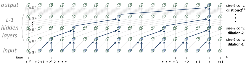
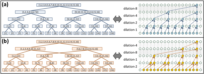
The dilated convolutional network we consider as baseline is the one underlying WaveNet, depicted in fig. 7. It is a 1D convolutional network without pooling, whose convolutional filters are dilated, i.e. incorporate gaps between their elements. Each layer is characterized by a different dilation, twice as large as that of its preceding layer. As before, we study functions realized by networks through the hierarchical decompositions that represent their grid tensors (see sec. 3). In the case of the baseline dilated convolutional network, the hierarchical decomposition adheres to a tree over tensor modes as illustrated in fig. 8(a). Modifying the structure of this tree yields a hierarchical decomposition that corresponds to a network with modified dilations throughout its layers – see illustration of a particular example in fig. 8(b).
For the analysis of networks with different connectivity schemes, we introduce the notion of mixed tensor decompositions. Let and be two dilated convolutional networks whose corresponding hierarchical tensor decompositions are based on mode trees and (respectively). The mixed tensor decomposition of and runs their hierarchical decompositions in parallel, while exchanging tensors at different points along the way. It represents the grid tensors of a mixed network , obtained by interconnecting the intermediate layers of and .
We would like to show that is expressively efficient with respect to and , thereby exemplifying the ability of interconnectivity to introduce efficiency. As discussed in sec. 2, this requires proving two propositions:
-
(i)
Any function realized by or can be replicated by with no more than linear growth in size
-
(ii)
There exist functions realized by that cannot be replicated by or unless their size is allowed to grow super-linearly
Proposition (i) follows from the fact that the mixed network reduces to one of the networks it comprises ( or ) if we set the opposite network’s weights to zero. For proposition (ii), we compare matricization ranks under the hierarchical decompositions of and , to those brought forth by their mixture. This results in the following theorem (see [Cohen et al.(2017)Cohen, Tamari, and Shashua] for proof):
Theorem 8.1.
Let and be different trees over tensor modes, and consider the hierarchical decompositions they give rise to. These decompositions must grow (in terms of the number of intermediate tensors – sec. 3) at least quadratically to replicate tensors generated by their mixture.
From a network perspective, theorem 8.1 translates to:
Corollary 8.2.
Let and be different dilated convolutional networks, and let be a network obtained by interconnecting their intermediate layers. realizes functions that cannot be replicated by or unless these are at least quadratically larger.
We conclude that with dilated convolutional networks, interconnectivity brings forth expressive efficiency. Moreover, even a single connection between intermediate layers of different networks already leads to a quadratic gap, which in large-scale settings typically makes the difference between a model that is practical and one that is not. Empirical evaluation of the analyzed models (carried out in [Cohen et al.(2017)Cohen, Tamari, and Shashua]) demonstrates how adding connections between intermediate layers of different networks improves accuracy, with no additional cost in terms of computation or model capacity. This serves as yet another indication that in general, expressive efficiency and improved accuracies go hand in hand.
9 Conclusion
Expressive efficiency and inductive bias are the primary notions for formally reasoning about expressiveness – the driving force behind convolutional networks. Perhaps more important than their role in formalizing common beliefs and explaining empirically observed phenomena, is the potential of expressive efficiency and inductive bias to provide new tools for network design. Expressive efficiency can be viewed as the enhancement of a network’s expressiveness, whereas inductive bias corresponds to making better use of expressive resources given the needs of a task at hand. Mounting empirical evidence shows time and time again that both procedures directly lead to improved performance (accuracies in particular).
Through an equivalence to hierarchical tensor decompositions, we analyzed the expressive efficiency and inductive bias of various architectural features in convolutional networks. Specifically, we studied the effects of network depth, layer widths, geometry of pooling windows, overlapping convolutions, and interconnectivity schemes. The results derived are not only explanatory – they provide concrete steps for controlling expressive efficiency and inductive bias. For example, guidelines are given for setting layer widths and pooling geometries in accordance with input correlations one wishes to model. We hope the series of works reviewed in this paper will serve as a first step towards extensive use of hierarchical tensor decompositions for more principled convolutional network design.
Acknowledgements.
References
References
- [Beylkin and Mohlenkamp(2002)] Gregory Beylkin and Martin J Mohlenkamp. Numerical operator calculus in higher dimensions. Proceedings of the National Academy of Sciences, 99(16):10246–10251, 2002.
- [Cohen and Shashua(2016)] Nadav Cohen and Amnon Shashua. Convolutional rectifier networks as generalized tensor decompositions. International Conference on Machine Learning (ICML), 2016.
- [Cohen and Shashua(2017)] Nadav Cohen and Amnon Shashua. Inductive bias of deep convolutional networks through pooling geometry. International Conference on Learning Representations (ICLR), 2017.
- [Cohen et al.(2016a)Cohen, Sharir, and Shashua] Nadav Cohen, Or Sharir, and Amnon Shashua. Deep simnets. IEEE Conference on Computer Vision and Pattern Recognition (CVPR), 2016a.
- [Cohen et al.(2016b)Cohen, Sharir, and Shashua] Nadav Cohen, Or Sharir, and Amnon Shashua. On the expressive power of deep learning: A tensor analysis. Conference On Learning Theory (COLT), 2016b.
- [Cohen et al.(2017)Cohen, Tamari, and Shashua] Nadav Cohen, Ronen Tamari, and Amnon Shashua. Boosting dilated convolutional networks with mixed tensor decompositions. arXiv preprint arXiv:1703.06846, 2017.
- [Cui et al.(2016)Cui, Freedman, Sattath, Stong, and Minton] Shawn X Cui, Michael H Freedman, Or Sattath, Richard Stong, and Greg Minton. Quantum max-flow/min-cut. Journal of Mathematical Physics, 57(6):062206, 2016.
- [Delalleau and Bengio(2011)] Olivier Delalleau and Yoshua Bengio. Shallow vs. deep sum-product networks. In Advances in Neural Information Processing Systems, pages 666–674, 2011.
- [Eldan and Shamir(2015)] Ronen Eldan and Ohad Shamir. The power of depth for feedforward neural networks. arXiv preprint arXiv:1512.03965, 2015.
- [Hackbusch and Kühn(2009)] W Hackbusch and S Kühn. A New Scheme for the Tensor Representation. Journal of Fourier Analysis and Applications, 15(5):706–722, 2009.
- [Hackbusch(2012)] Wolfgang Hackbusch. Tensor Spaces and Numerical Tensor Calculus, volume 42 of Springer Series in Computational Mathematics. Springer Science & Business Media, Berlin, Heidelberg, February 2012.
- [He et al.(2015)He, Zhang, Ren, and Sun] Kaiming He, Xiangyu Zhang, Shaoqing Ren, and Jian Sun. Deep residual learning for image recognition. arXiv preprint arXiv:1512.03385, 2015.
- [Huang et al.(2016)Huang, Liu, Weinberger, and van der Maaten] Gao Huang, Zhuang Liu, Kilian Q Weinberger, and Laurens van der Maaten. Densely connected convolutional networks. arXiv preprint arXiv:1608.06993, 2016.
- [Jia et al.(2014)Jia, Shelhamer, Donahue, Karayev, Long, Girshick, Guadarrama, and Darrell] Yangqing Jia, Evan Shelhamer, Jeff Donahue, Sergey Karayev, Jonathan Long, Ross Girshick, Sergio Guadarrama, and Trevor Darrell. Caffe: Convolutional architecture for fast feature embedding. In Proceedings of the 22nd ACM international conference on Multimedia, pages 675–678. ACM, 2014.
- [Kalchbrenner et al.(2016)Kalchbrenner, Espeholt, Simonyan, Oord, Graves, and Kavukcuoglu] Nal Kalchbrenner, Lasse Espeholt, Karen Simonyan, Aaron van den Oord, Alex Graves, and Koray Kavukcuoglu. Neural machine translation in linear time. arXiv preprint arXiv:1610.10099, 2016.
- [Kolda and Bader(2009)] Tamara G Kolda and Brett W Bader. Tensor Decompositions and Applications. SIAM Review (), 51(3):455–500, 2009.
- [Krizhevsky et al.(2012)Krizhevsky, Sutskever, and Hinton] Alex Krizhevsky, Ilya Sutskever, and Geoffrey E Hinton. ImageNet Classification with Deep Convolutional Neural Networks. Advances in Neural Information Processing Systems, pages 1106–1114, 2012.
- [LeCun and Bengio(1995)] Yann LeCun and Yoshua Bengio. Convolutional networks for images, speech, and time series. The handbook of brain theory and neural networks, 3361(10), 1995.
- [LeCun et al.(2015)LeCun, Bengio, and Hinton] Yann LeCun, Yoshua Bengio, and Geoffrey Hinton. Deep learning. Nature, 521(7553):436–444, May 2015.
- [Levine et al.(2017)Levine, Yakira, Cohen, and Shashua] Yoav Levine, David Yakira, Nadav Cohen, and Amnon Shashua. Deep learning and quantum entanglement: Fundamental connections with implications to network design. arXiv preprint arXiv:1704.01552, 2017.
- [Li et al.(2017)Li, Li, Fern, and Raich] Xingyi Li, Fuxin Li, Xiaoli Fern, and Raviv Raich. Filter shaping for convolutional neural networks. International Conference on Learning Representations (ICLR), 2017.
- [Mhaskar et al.(2016)Mhaskar, Liao, and Poggio] Hrushikesh Mhaskar, Qianli Liao, and Tomaso Poggio. Learning real and boolean functions: When is deep better than shallow. arXiv preprint arXiv:1603.00988, 2016.
- [Montufar et al.(2014)Montufar, Pascanu, Cho, and Bengio] Guido F Montufar, Razvan Pascanu, Kyunghyun Cho, and Yoshua Bengio. On the number of linear regions of deep neural networks. In Advances in Neural Information Processing Systems, pages 2924–2932, 2014.
- [Nair and Hinton(2010)] Vinod Nair and Geoffrey E Hinton. Rectified linear units improve restricted boltzmann machines. In Proceedings of the 27th International Conference on Machine Learning (ICML-10), pages 807–814, 2010.
- [Orús(2014)] Román Orús. A practical introduction to tensor networks: Matrix product states and projected entangled pair states. Annals of Physics, 349:117–158, 2014.
- [Pascanu et al.(2013)Pascanu, Montufar, and Bengio] Razvan Pascanu, Guido Montufar, and Yoshua Bengio. On the number of inference regions of deep feed forward networks with piece-wise linear activations. arXiv preprint arXiv, 1312, 2013.
- [Plenio and Virmani(2007)] MARTIN B Plenio and SHASHANK Virmani. An introduction to entanglement measures. Quantum Information and Computation, 7(1):001–051, 2007.
- [Poggio et al.(2015)Poggio, Anselmi, and Rosasco] Tomaso Poggio, Fabio Anselmi, and Lorenzo Rosasco. I-theory on depth vs width: hierarchical function composition. Technical report, Center for Brains, Minds and Machines (CBMM), 2015.
- [Poon and Domingos(2011)] Hoifung Poon and Pedro Domingos. Sum-product networks: A new deep architecture. In Computer Vision Workshops (ICCV Workshops), 2011 IEEE International Conference on, pages 689–690. IEEE, 2011.
- [Rosenblatt(1961)] Frank Rosenblatt. Principles of neurodynamics. perceptrons and the theory of brain mechanisms. Technical report, DTIC Document, 1961.
- [Sharir and Shashua(2017)] Or Sharir and Amnon Shashua. On the expressive power of overlapping operations of deep networks. arXiv preprint arXiv:1703.02065, 2017.
- [Sharir et al.(2017)Sharir, Tamari, Cohen, and Shashua] Or Sharir, Ronen Tamari, Nadav Cohen, and Amnon Shashua. Tensorial mixture models. arXiv preprint arXiv:1610.04167, 2017.
- [Simonyan and Zisserman(2014)] Karen Simonyan and Andrew Zisserman. Very deep convolutional networks for large-scale image recognition. arXiv preprint arXiv:1409.1556, 2014.
- [Szegedy et al.(2015)Szegedy, Liu, Jia, Sermanet, Reed, Anguelov, Erhan, Vanhoucke, and Rabinovich] Christian Szegedy, Wei Liu, Yangqing Jia, Pierre Sermanet, Scott Reed, Dragomir Anguelov, Dumitru Erhan, Vincent Vanhoucke, and Andrew Rabinovich. Going Deeper with Convolutions. CVPR, 2015.
- [Szegedy et al.(2016)Szegedy, Vanhoucke, Ioffe, Shlens, and Wojna] Christian Szegedy, Vincent Vanhoucke, Sergey Ioffe, Jon Shlens, and Zbigniew Wojna. Rethinking the inception architecture for computer vision. In Proceedings of the IEEE Conference on Computer Vision and Pattern Recognition, pages 2818–2826, 2016.
- [Telgarsky(2015)] Matus Telgarsky. Representation benefits of deep feedforward networks. arXiv preprint arXiv:1509.08101, 2015.
- [van den Oord et al.(2016)van den Oord, Dieleman, Zen, Simonyan, Vinyals, Graves, Kalchbrenner, Senior, and Kavukcuoglu] Aäron van den Oord, Sander Dieleman, Heiga Zen, Karen Simonyan, Oriol Vinyals, Alex Graves, Nal Kalchbrenner, Andrew Senior, and Koray Kavukcuoglu. Wavenet: A generative model for raw audio. CoRR abs/1609.03499, 2016.
- [Yu and Koltun(2015)] Fisher Yu and Vladlen Koltun. Multi-scale context aggregation by dilated convolutions. arXiv preprint arXiv:1511.07122, 2015.