Non-stationary spin-filtering effects in correlated quantum dot

Abstract

The influence of external magnetic field switching $"$on$"$ and $"$off$"$ on the non-stationary spin-polarized currents in the system of correlated single-level quantum dot coupled to non-magnetic electronic reservoirs has been analyzed. It was shown that considered system can be used for the effective spin filtering by analyzing its non-stationary characteristics in particular range of applied bias voltage.

I Introduction

One of the key issues of spintronics is the control and generation of spin-polarized currents. Nowadays generation and detection of spin-polarized currents in semiconductor nanostructures has attracted great attention since this is the key problem in developing semiconductor spintronic devices Awschalom ,Prinz , Crook ,Chuang . To generate tunable highly spin-polarized stationary currents the variety of systems has been already proposed ranging from semiconductor heterostructures to low-dimensional mesoscopic samples Kagan ,Zutic ,Torio ,Shakirov . Significant progress has been achieved in experimental and theoretical investigation of stationary spin-polarized transport in magnetic tunneling junctions Tsymbal ,Zhu ,Ohno ,Fiederling . Nevertheless spin-polarized current sources based on the non-magnetic materials are attractable as one could avoid the presence of accidental magnetic fields that may result in the existence of undesirable effects on the spin currents. It was demonstrated recently that stationary tunneling current could be spin dependent in the case of non-magnetic leads Perel' , Glazov . There have been several proposals to generate stationary spin-polarized currents using non-magnetic materials: small quantum dots Recher ,Potok and coupled quantum dots Kagan ,Andrade built in semiconducting nanostructures in the presence of external magnetic field. Moreover, quantum dots systems based on the non-magnetic materials were proposed as a spin filter prototypes Koga , Voskoboynikov . Effective spin filtering in such systems requires to have many quantum dots with the Coulomb correlations inside each dot Gong ,Ojeda ,Fu and also between the dots Kagan .

To the best of our knowledge usually stationary spin-polarized currents are analyzed. However, creation, diagnostics and controllable manipulation of charge and spin states in the single and coupled quantum dots (QDs), applicable for ultra small size electronic devices design requires analysis of non-stationary effects and transient processes Bar-Joseph ,Gurvitz_1 , Arseyev_1 ,Stafford_1 ,Hazelzet ,Cota . Consequently, non-stationary evolution of initially prepared spin and charge configurations in correlated quantum dots is of great interest both from fundamental and technological point of view.

In this paper we analyze non-stationary spin polarized currents through the correlated single-level QD localized in the tunnel junction in the presence of applied bias voltage and external magnetic field, which can be switched $"$on$"$ or $"$off$"$ at a particular time moment. We demonstrate that single biased QD in the external magnetic field can be considered as an effective spin filter based on the analysis of non-stationary spin-polarized currents, which can flow in the both leads. Currents direction can be tuned by the external magnetic field switching $"$on$"$ or $"$off$"$.

II Theoretical model

We consider non-stationary processes in the single-level quantum dot with Coulomb correlations of localized electrons situated between two non-magnetic electronic reservoirs in the presence of external magnetic field B switched $"$on$"$/$"$off$"$ at $t=t_{0}$. The Hamiltonian of the system

$$\hat{H}=\hat{H}_{QD}+\hat{H}_{R}+\hat{H}_{T}$$ (1)

can be written as a sum of the single-level quantum dot part

$$\hat{H}_{QD}=\sum_{\sigma}\varepsilon_{1}\hat{n}_{1}^{\sigma}++U\hat{n}_{1}^{\sigma}\hat{n}_{1}^{-\sigma},$$ (2)

non-magnetic electronic reservoirs Hamiltonian

$$\hat{H}_{R}=\sum_{k\sigma}\varepsilon_{k}\hat{c}_{k\sigma}^{+}\hat{c}_{k\sigma}+\sum_{p\sigma}(\varepsilon_{p}-eV)\hat{c}_{p\sigma}^{+}\hat{c}_{p\sigma}$$ (3)

and the tunneling part

$$\hat{H}_{T}=\sum_{k\sigma}t_{k}(\hat{c}_{k\sigma}^{+}\hat{c}_{1\sigma}+\hat{c}_{1\sigma}^{+}\hat{c}_{k\sigma})+\sum_{p\sigma}t_{p}(\hat{c}_{p\sigma}^{+}\hat{c}_{1\sigma}+\hat{c}_{1\sigma}^{+}\hat{c}_{p\sigma}).$$

Here index $k(p)$ labels continuous spectrum states in the leads, $t_{k(p)}$ is the tunneling transfer amplitude between continuous spectrum states and quantum dot with the energy level $\varepsilon_{1}$ which is considered to be independent on the momentum and spin. Operators $\hat{c}_{k(p)\sigma}^{+}/\hat{c}_{k(p)\sigma}$ are the creation/annihilation operators for the electrons in the continuous spectrum states $k(p)$. $\hat{n}_{1}^{\sigma(-\sigma)}=\hat{c}_{1\sigma(-\sigma)}^{+}\hat{c}_{1\sigma(-\sigma)}$-localized state electron occupation numbers, where operator $\hat{c}_{1\sigma(-\sigma)}$ destroys electron with spin $\sigma(-\sigma)$ on the energy level $\varepsilon_{1}$. $U$ is the on-site Coulomb repulsion for the double occupation of the quantum dot. External magnetic field B leads to the Zeeman splitting of the impurity single level $\varepsilon_{1}$ proportional to the atomic $g$ factor. Further analysis deals with the low temperature regime when the Fermi level is well defined and the temperature is much lower than all the typical energy scales in the system. Consequently, the distribution function of electrons in the leads (band electrons) is close to the Fermi step.

III Non-stationary electronic transport formalism

Let us further consider $\hbar=1$ and $e=1$ elsewhere, so the motion equations for the electron operators products $\hat{n}_{1}^{\sigma}$, $\hat{n}_{1k}^{\sigma}=\hat{c}_{1\sigma}^{+}\hat{c}_{k\sigma}$ and $\hat{c}_{k^{{}^{\prime}}\sigma}^{+}\hat{c}_{k\sigma}$ can be written as:

$$i\frac{\partial\hat{n}_{1}^{\sigma}}{\partial t}= - \sum_{k,\sigma}t_{k}\cdot(\hat{n}_{k1}^{\sigma}-\hat{n}_{1k}^{\sigma}),$$ (5)

$$i\frac{\partial\hat{n}_{1k}^{\sigma}}{\partial t}= - (\varepsilon_{1}^{\sigma}-\varepsilon_{k})\cdot\hat{n}_{1k}^{\sigma}-U\cdot\hat{n}_{1}^{-\sigma}\hat{n}_{1k}^{\sigma}+$$ (6)

$$+ t_{k}\cdot(\hat{n}_{1}^{\sigma}-\hat{n}_{k}^{\sigma})-\sum_{k^{{}^{\prime}}\neq k}t_{k^{{}^{\prime}}}\cdot\hat{c}_{k^{{}^{\prime}}\sigma}^{+}\hat{c}_{k\sigma},$$

$$i\frac{\partial\hat{c}_{k^{{}^{\prime}}\sigma}^{+}\hat{c}_{k\sigma}}{\partial t}= - (\varepsilon_{k^{{}^{\prime}}}-\varepsilon_{k})\cdot\hat{c}_{k^{{}^{\prime}}\sigma}^{+}\hat{c}_{k\sigma}-$$ (7)

$$- t_{k^{{}^{\prime}}}\cdot\hat{c}_{1\sigma}^{+}\hat{c}_{k\sigma}+t_{k}\cdot\hat{c}_{k^{{}^{\prime}}\sigma}^{+}\hat{c}_{1\sigma}.$$

and

$$i\frac{\partial\hat{c}_{p\sigma}^{+}\hat{c}_{k\sigma}}{\partial t} = (\varepsilon_{k}-\varepsilon_{p})\cdot\hat{c}_{p\sigma}^{+}\hat{c}_{k\sigma}+$$ (8)

$$+ t_{k}\cdot\hat{c}_{p\sigma}^{+}\hat{c}_{1\sigma}-t_{p}\cdot\hat{c}_{1\sigma}^{+}\hat{c}_{k\sigma},$$

where $\hat{n}_{k}^{\sigma}=\hat{c}_{k\sigma}^{+}\hat{c}_{k\sigma}$ is an occupation operator for the electrons in the reservoir and $\varepsilon_{\sigma}=\varepsilon_{1}+\sigma\mu B$ where $\sigma=\pm 1$. Equations of motion for the electron operators products $\hat{c}_{1\sigma}^{+}\hat{c}_{p\sigma}$ and $\hat{c}_{p^{{}^{\prime}}\sigma}^{+}\hat{c}_{p\sigma}$ can be obtained from Eq.(6) and Eq.(7) correspondingly by the indexes substitution $k\leftrightarrow p$ and $k^{{}^{\prime}}\leftrightarrow p^{{}^{\prime}}$.

Following the logic of Ref. Maslova one can get kinetic equations for the electron occupation numbers operators time evolution in the case of external magnetic field B switching $"$on$"$ at the time moment $t=t_{0}>0$:

$$\frac{\partial n_{1}^{\sigma}}{\partial t}=-2\Theta(t_{0}-t)\cdot\gamma\times$$

$$\times[n_{1}^{\sigma}-(1-n_{1}^{-\sigma})\cdot\Phi_{\varepsilon}^{T}(t)-n_{1}^{-\sigma}\cdot\Phi_{\varepsilon+U}^{T}(t)]-$$

$$-2\Theta(t-t_{0})\cdot\gamma\times$$

$$\times[n_{1}^{\sigma}-(1-n_{1}^{-\sigma})\cdot\Phi_{\varepsilon}^{+T}(t)-n_{1}^{-\sigma}\cdot\Phi_{\varepsilon+U}^{+T}(t)],$$

$$\frac{\partial n_{1}^{-\sigma}}{\partial t}=-2\Theta(t_{0}-t)\cdot\gamma\times$$

$$\times[n_{1}^{-\sigma}-(1-n_{1}^{\sigma})\cdot\Phi_{\varepsilon}^{T}(t)-n_{1}^{\sigma}\cdot\Phi_{\varepsilon+U}^{T}(t)]-$$

$$-2\Theta(t-t_{0})\cdot\gamma\times$$

$$\times[n_{1}^{-\sigma}-(1-n_{1}^{\sigma})\cdot\Phi_{\varepsilon}^{-T}(t)-n_{1}^{\sigma}\cdot\Phi_{\varepsilon+U}^{-T}(t)],$$

(9)

where $\gamma=\gamma_{k}+\gamma_{p}$ and $\gamma_{k(p)}=\pi\nu_{0}t_{k(p)}^{2}$. $\nu_{0}$ - is the unperturbed density of states in the leads and

$$\hat{\Phi}_{\varepsilon}^{\pm T}(t) = \frac{\gamma_{k}}{\gamma}\cdot\hat{\Phi}^{\pm}_{k\varepsilon}(t)+\frac{\gamma_{p}}{\gamma}\cdot\hat{\Phi}^{\pm}_{p\varepsilon}(t),$$

$$\hat{\Phi}_{\varepsilon+U}^{\pm T}(t) = \frac{\gamma_{k}}{\gamma}\cdot\hat{\Phi}^{\pm}_{k\varepsilon+U}(t)+\frac{\gamma_{p}}{\gamma}\cdot\hat{\Phi}^{\pm}_{p\varepsilon+U}(t),$$

where

$$\hat{\Phi}_{\varepsilon}^{\pm}(t)=\frac{1}{2}i\cdot\int d\varepsilon_{k}\cdot f_{k}^{\sigma}(\varepsilon_{k})\times$$

$$\times[\frac{1-e^{i(\varepsilon_{1}\pm\mu B+i\Gamma-\varepsilon_{k})t}}{\varepsilon_{1}\pm\mu B+i\Gamma-\varepsilon_{k}}-\frac{1-e^{-i(\varepsilon_{1}\pm\mu B-i\Gamma-\varepsilon_{k})t}}{\varepsilon_{1}\pm\mu B-i\Gamma-\varepsilon_{k}}],$$

$$\hat{\Phi}_{\varepsilon+U}^{\pm}(t)=\frac{1}{2}i\cdot\int d\varepsilon_{k}\cdot f_{k}^{\sigma}(\varepsilon_{k})\times$$

$$\times[\frac{1-e^{i(\varepsilon_{1}\pm\mu B+U+i\Gamma-\varepsilon_{k})t}}{\varepsilon_{1}\pm\mu B+U+i\Gamma-\varepsilon_{k}}-\frac{1-e^{-i(\varepsilon_{1}\pm\mu B+U-i\Gamma-\varepsilon_{k})t}}{\varepsilon_{1}\pm\mu B+U-i\Gamma-\varepsilon_{k}}].$$

(11)

Initially ($t<t_{0}$) magnetic field B is absent [$\mu B=0$ in Eqs.(9)-(11)] and, consequently, the following relation is valid $\hat{\Phi}_{\varepsilon}^{\pm}(t)=\hat{\Phi}_{\varepsilon}(t)$. To analyze system kinetics in the situation when magnetic field was initially present in the system and switched $"$off$"$ at $t=t_{0}$ one can easily generalize Eqs.(9) by substitution $t\leftrightarrow t_{0}$.

Equations for the localized electrons occupation numbers $n_{1\pm}^{\sigma}(t)$ can be obtained by averaging Eqs. (9)-(11) for the operators and by decoupling electrons occupation numbers in the leads. Such decoupling procedure is reasonable if one considers that electrons in the macroscopic leads are in the thermal equilibrium You ; Zheng . After decoupling one has to replace electron occupation numbers operators in the reservoir $\hat{n}_{k}^{\sigma}$ in Eqs. (9)-(11) by the Fermi distribution functions $f_{k}^{\sigma}$.

IV Non-stationary spin-polarized currents

If the initial state is a $"$magnetic$"$ one, non-stationary spin-polarized currents $I_{k(p)}(t)^{\pm}$ flow in the each contact lead:

$$I_{k}^{\pm}(t) = -2\gamma_{k}\cdot[n_{1}^{\pm\sigma}-(1-n_{1}^{\mp\sigma})\cdot\Phi_{k\varepsilon}^{\pm}(t)-n_{1}^{\mp\sigma}\cdot\Phi_{k\varepsilon+U}^{\pm}(t)]-$$

$$- 2\gamma_{k}\cdot[n_{1}^{\pm\sigma}-(1-n_{1}^{\mp\sigma})\cdot\Phi_{k\varepsilon}(t)-n_{1}^{\mp\sigma}\cdot\Phi_{k\varepsilon+U}(t)],$$

$$I_{p}^{\pm}(t) = -2\gamma_{p}\cdot[n_{1}^{\pm\sigma}-(1-n_{1}^{\mp\sigma})\cdot\Phi_{p\varepsilon}^{\pm}(t)-n_{1}^{\mp\sigma}\cdot\Phi_{p\varepsilon+U}^{\pm}(t)]-$$

$$- 2\gamma_{p}\cdot[n_{1}^{\pm\sigma}-(1-n_{1}^{\mp\sigma})\cdot\Phi_{p\varepsilon}(t)-n_{1}^{\mp\sigma}\cdot\Phi_{p\varepsilon+U}(t)],$$

where electron occupation numbers $n_{1}^{\pm\sigma}$ are determined from the system of Equations (9) with the magnetic initial conditions.

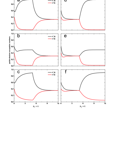
Figure 1: (Color online) Occupation numbers time evolution. Panels a)-c) correspond to the magnetic field switching $"$on$"$, panels d)-f)correspond to the magnetic field switching $"$off$"$. a),d) $\varepsilon_{1}/2\gamma=-1.25$, $eV/2\gamma=-2.5$; b),e) $\varepsilon_{1}/2\gamma=-1.25$, $eV/2\gamma=-7.5$; c),f) $\varepsilon_{1}/2\gamma=-5$, $eV/2\gamma=-6.25$. Parameters $U/2\gamma=10$, $\mu B/2\gamma=-3.25$, $\gamma_{k}=\gamma_{p}=\gamma=1$ and initial conditions $n_{1}^{\sigma}(0)=0.6$, $n_{1}^{-\sigma}(0)=0.4$ are the same for all the figures.

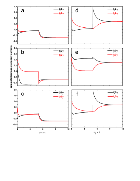
Figure 2: (Color online) Normalized non-stationary spin-polarized tunneling currents $I_{k(p)^{\pm}(t)}/2\gamma$ in the case of magnetic field switching $"$off$"$ at $t=t_{0}$. Panels a)-c) demonstrate $I_{k^{\pm}(t)}/2\gamma$, panels d)-f)demonstrate $I_{p^{\pm}(t)}/2\gamma$. a),d) $\varepsilon_{1}/2\gamma=-1.25$, $eV/2\gamma=-2.5$; b),e) $\varepsilon_{1}/2\gamma=-1.25$, $eV/2\gamma=-7.5$; c),f) $\varepsilon_{1}/2\gamma=-5$, $eV/2\gamma=-6.25$. Parameters $U/2\gamma=10$, $\mu B/2\gamma=-3.25$, $\gamma_{k}=\gamma_{p}=\gamma=1$ and initial conditions $n_{1}^{\sigma}(0)=0.6$, $n_{1}^{-\sigma}(0)=0.4$ are the same for all the figures.

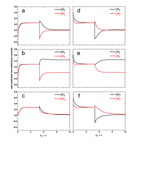
Figure 3: (Color online) Normalized non-stationary spin-polarized tunneling currents $I_{k(p)^{\pm}(t)}/2\gamma$ in the case of magnetic field switching $"$on$"$ at $t=t_{0}$. Panels a)-c) demonstrate $I_{k^{\pm}(t)}/2\gamma$, panels d)-f)demonstrate $I_{p^{\pm}(t)}/2\gamma$. a),d) $\varepsilon_{1}/2\gamma=-1.25$, $eV/2\gamma=-2.5$; b),e) $\varepsilon_{1}/2\gamma=-1.25$, $eV/2\gamma=-7.5$; c),f) $\varepsilon_{1}/2\gamma=-5$, $eV/2\gamma=-6.25$. Parameters $U/2\gamma=10$, $\mu B/2\gamma=-3.25$, $\gamma_{k}=\gamma_{p}=\gamma=1$ and initial conditions $n_{1}^{\sigma}(0)=0.6$, $n_{1}^{-\sigma}(0)=0.4$ are the same for all the figures.

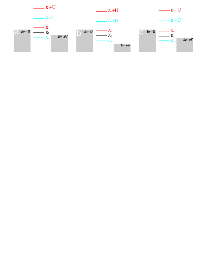
Figure 4: (Color online) Sketch of the correlated QD energy levels coupled to non-magnetic leads both in the presence ($\varepsilon_{+}$ and $\varepsilon_{-}$) and in the absence ($\varepsilon_{1}$) of magnetic field.

Non-stationary spin-polarized currents can flow in the both leads and their direction and polarization can be tuned by magnetic field B switching $"$on$"$/$"$off$"$. Non-stationary spin-polarized currents $I_{k(p)}^{\pm}(t)$ behavior for magnetic field switching $"$on$"$/$"$off$"$ is shown in Figs.2-3. Corresponding electron occupation numbers behavior is depicted in Fig.1. Schemes of the QD energy levels both in the presence ($\varepsilon_{+}$ and $\varepsilon_{-}$) and in the absence ($\varepsilon_{1}$) of magnetic field are shown in Fig.4. Let us first focus on the situation when magnetic field is present at the initial time moment and switched $"$off$"$ at $t=t_{0}$ (see Fig.1a,c,e and Fig.2). In the presence of magnetic field when condition $\varepsilon_{+}<E_{F}-eV$ occurs (energy level $\varepsilon_{-}$ can be localized higher or lower than $E_{F}$) (see Fig.4a,c), non-stationary spin-polarized currents $I_{k}^{-}(t)$ and $I_{k}^{+}(t)$ in the lead with $E_{F}=0$ are flowing in the same direction (see Fig.2a,c), contrary to the currents $I_{p}^{-}(t)$ and $I_{p}^{+}(t)$ flowing in the opposite directions in the lead with the Fermi level shifted by the applied bias voltage (lead $p$) (see Fig.2d,f). In the stationary state all currents $I_{k(p)}^{\pm}(t)$ values turn to zero. Magnetic field switching $"$off$"$ results in the appearance of non-zero spin-polarized currents in both leads. Non-stationary spin-polarized currents $I_{k}^{-}(t)$ and $I_{k}^{+}(t)$ in the lead with $E_{F}=0$ continue flowing in the same direction with the same non-zero amplitude (see Fig.2a,c). Currents $I_{p}^{-}(t)$ and $I_{p}^{+}(t)$ are also flowing in the same direction but magnetic field switching $"$off$"$ results in the appearance of total current strong spin polarization at the initial stage of relaxation as the amplitude of current $I_{p}^{+}(t)$ strongly exceeds the amplitude of non-stationary current $I_{p}^{-}(t)$ (see Fig.2d,f). Similar behavior of electron occupation numbers and non-stationary spin-polarized currents for two different positions of $\varepsilon_{-}$ (see Fig.4a,c) is the result of the Coulomb correlations presence in the system. In both cases energy level $\varepsilon_{+}$ is occupied and energy level $\varepsilon_{-}$ is unoccupied (even in the case depicted in Fig.4c) due to the strong Coulomb repulsion. Non-stationary current $I_{p}^{+}(t)$ changes direction with the magnetic field switching $"$off$"$, while currents $I_{k}^{\pm}(t)$ and $I_{p}^{-}(t)$ are flowing in the same direction both in presence and in the absence of magnetic field. This effect can be applied for the effective spin-filtering in the single QD system alternatively to the previously proposed spin-filtering mechanisms based on the analysis of multiple QDs stationary characteristics Kagan . Figure4b demonstrates that in the presence of magnetic field at the initial stage of relaxation non-stationary spin-polarized currents $I_{k}^{\pm}(t)$ can flow in the opposite directions and currents $I_{p}^{\pm}(t)$ in the same directions (see Fig.2b,e). Stationary state reveals the presence of only one non-stationary current flowing in each lead ($I_{k}^{+}(t)$ and $I_{p}^{+}(t)$ correspondingly). Magnetic field switching $"$off$"$ causes the appearance of both spin-polarized currents $I_{k}^{\pm}(t)$ and $I_{p}^{\pm}(t)$ flowing in each lead in the same direction. In the stationary state spin currents values in each lead become equal.

Electron occupation numbers and non-stationary spin-polarized currents behavior in the case when magnetic field is absent at the initial time moment and switched $"$on$"$ at $t=t_{0}$ is shown in Fig.1b,d,f and Fig.3 correspondingly. Obtained results demonstrate that magnetic field switching $"$on$"$ allows to consider single QD as an effective spin-filter based on the analysis of its non-stationary characteristics. In the absence of magnetic field non-stationary spin-polarized currents in each lead $I_{k}^{\pm}(t)$ and $I_{p}^{\pm}(t)$ are flowing in the same direction and demonstrate equal non-zero stationary values (see Fig.3). Magnetic field switching $"$on$"$ results in the direction changing of one of the spin-polarized currents in the leads (see Fig.3a,d,f). Another possible situation deals with fast switching $"$off$"$ of one of the spin-polarized currents in each lead when magnetic field is switched $"$on$"$ ( see Fig.3b,e). Consequently, only non-stationary current with a certain spin orientation continue flowing in each lead in the presence of magnetic field.

To observe these effects the switching times of magnetic field must be smaller than the lifetime of the initially prepared magnetic states. Modern scanning tunneling microscopy/spectroscopy experiments provide possibility to achieve typical spin-polarized current values of the order of $10$ pA $\div 10$ nA ($1nA\simeq 6\times 10^{9}e/sec$) (Amaha ,Fransson ), which corresponds to the relaxation time scales $1/\Gamma\simeq 1\div 100$ nsec for the system parameters depicted in Fig.2, Fig.3.

V Conclusion

We have analyzed the behavior of spin-polarized non-stationary currents in the system of single-level quantum dot situated between two non-magnetic electronic reservoirs with Coulomb correlations of localized electrons in the presence of external magnetic field switched ”on” or ”off” at particular time moment. It was demonstrated that single-level correlated quantum dot can be considered as an effective spin filter depending on the ration between the values of magnetic field induced energy level splitting and applied bias voltage.

This work was supported by RFBR grant $16-32-60024$ $mol-a-dk$ and by the RF President Grant for young scientists $MD-4550.2016.2$.

References

(1)Semiconductor Spintronics and Quantum Computation, edited by
D.D. Awschalom, D. Loss, N. Samarth, Nanoscience and Technology
(Springer, Berlin, 2002).
(2)
G.A. Prinz, Science282, 1660, (1998)
(3)
R. Crook, J. Prance, K.J. Thomas, S.J. Chorley, I. Farrer, D.A.
Ritchie, M. Pepper, C.G. Smith, Science312, 1359,
(2006)
(4)
P. Chuang, S.C. Ho, L.W. Smith, F. Sfigakis, M. Pepper, C.H. Chen,
J.C. Fan, J.P. Griffits, I. Farrer, H.E. Beer, et.al., Nat.
Nanotechnology10, 35, (2015)