Sequential Attention:
A Context-Aware Alignment Function for Machine Reading

Abstract

In this paper we propose a neural network model with a novel Sequential Attention layer that extends soft attention by assigning weights to words in an input sequence in a way that takes into account not just how well that word matches a query, but how well surrounding words match. We evaluate this approach on the task of reading comprehension (on the Who did What and CNN datasets) and show that it dramatically improves a strong baseline—the Stanford Reader—and is competitive with the state of the art.

1 Introduction

Soft attention Bahdanau et al. (2014), a differentiable method for selecting the inputs for a component of a model from a set of possibilities, has been crucial to the success of artificial neural network models for natural language understanding tasks like reading comprehension that take short passages as inputs. However, standard approaches to attention in NLP select words with only very indirect consideration of their context, limiting their effectiveness. This paper presents a method to address this by adding explicit context sensitivity into the soft attention scoring function.

We demonstrate the effectiveness of this approach on the task of cloze-style reading comprehension. A problem in the cloze style consists of a passage p, a question q and an answer a drawn from among the entities mentioned in the passage. In particular, we use the CNN dataset Hermann et al. (2015), which introduced the task into widespread use in evaluating neural networks for language understanding, and the newer and more carefully quality-controlled Who did What dataset Onishi et al. (2016).

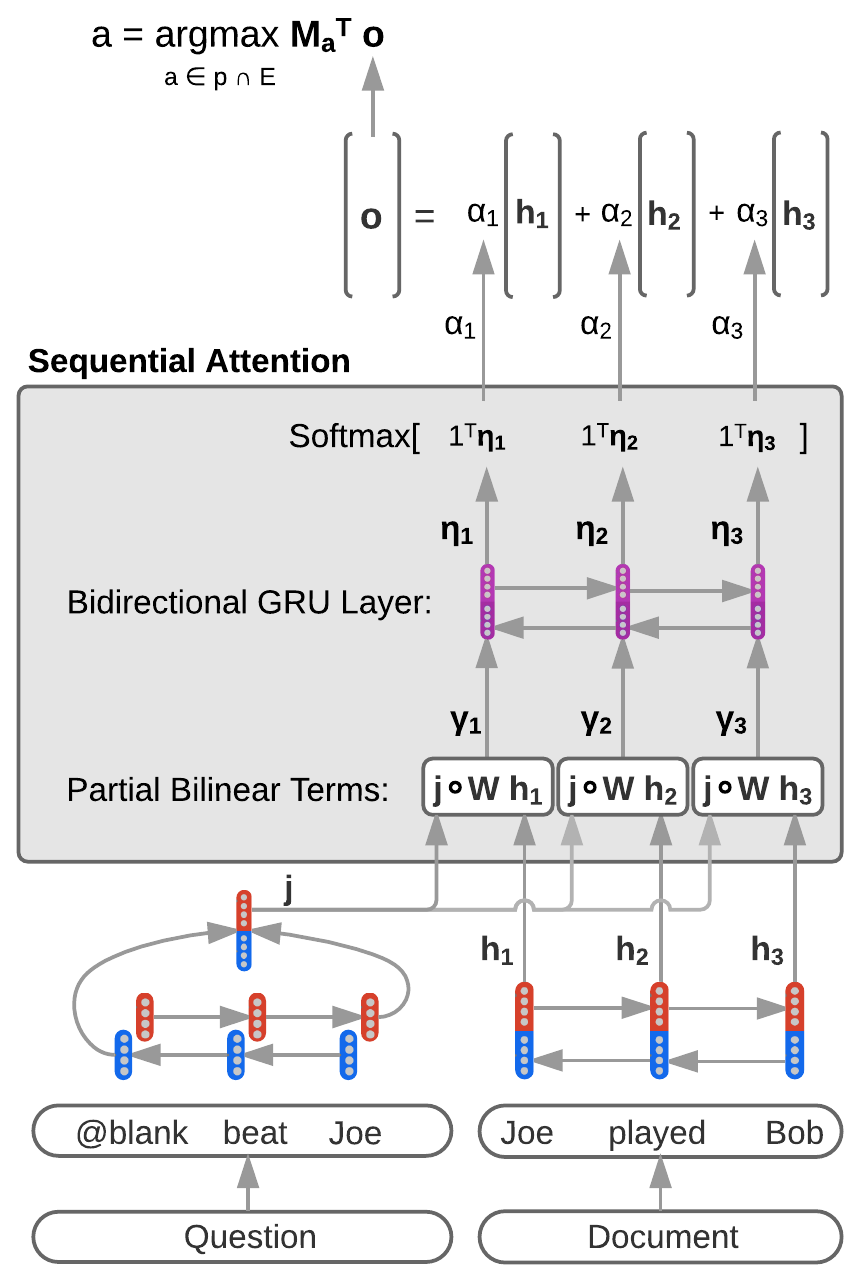
Figure 1: The Sequential Attention Model. RNNs first encode the question into a vector $\boldsymbol{j}$ and the document into a sequence of vectors $\boldsymbol{H}$. For each word index $i$ in the document, a scoring vector $\boldsymbol{\gamma_{i}}$ is then computed from $\boldsymbol{j}$ and $\boldsymbol{h_{i}}$ using a function like the partial bilinear function shown here. These vectors are then used as inputs to another RNN layer, the outputs of which ($\boldsymbol{\eta_{i}}$) are summed elementwise and used as attention scores ($\alpha_{i}$) in answer selection.

In standard approaches to soft attention over passages, a scoring function is first applied to every word in the source text to evaluate how closely that word matches a query vector (here, a function of the question). The resulting scores are then normalized and used as the weights in a weighted sum which produces an output or context vector summarizing the most salient words of the input, which is then used in a downstream model (here, to select an answer).

In this work we propose a novel scoring function for soft attention that we call Sequential Attention (SA), shown in Figure 1. In an SA model, a mutiplicative interaction scoring function is used to produce a scoring vector for each word in the source text. A newly-added bidirectional RNN then consumes those vectors and uses them to produce a context-aware scalar score for each word. We evaluate this scoring function within the context of the Stanford Reader Chen et al. (2016), and show that it yields dramatic improvements in performance. On both datasets, it is outperformed only by the Gated Attention Reader Dhingra et al. (2016), which in some cases has access to features not explicitly seen by our model.

2 Related Work

In addition to Chen et al. (2016)’s Stanford Reader model, there have been several other modeling approaches developed to address these reading comprehension tasks.

Seo et al. (2016) introduced the Bi-Directional Attention Flow which consists of a multi-stage hierarchical process to represent context at different levels of granularity; it use the concatenation of passage word representation, question word representation, and the element-wise product of these vectors in their attention flow layer. This is a more complex variant of the classic bi-linear term that multiplies this concatenated vector with a vector of weights, producing attention scalars. Dhingra et al. (2016)’s Gated-Attention Reader integrates a multi-hop structure with a novel attention mechanism, essentially building query specific representations of the tokens in the document to improve prediction. This model conducts a classic dot-product soft attention to weight the query representations which are then multiplied element-wise with the context representations, and fed into the next layer of RNN. After several hidden layers that repeat the same process, the dot product between the context representation and the query is used to compute a classic soft-attention.

Outside the task of reading comprehension there has been other work on soft attention over text, largely focusing on the problem of attending over single sentences. Luong et al. (2015) study several issues in the design of soft attention models in the context of translation, and introduce the bilinear scoring function. They also propose the idea of attention input-feeding where the original attention vectors are concatenated with the hidden representations of the words and fed into the next RNN step. The goal is to make the model fully aware of the previous alignment choices.

In work largely concurrent to our own, Kim et al. (2017) explore the use of conditional random fields (CRFs) to impose a variety of constraints on attention distributions achieving strong results on several sentence level tasks.

3 Modeling

Given the tuple (passage, question, answer), our goal is to predict $\Pr(a|d,q)$ where $a$ refers to answer, $d$ to passage, and $q$ to question. We define the words of each passage and question as $d={d_{1},..,d_{m}}$ and $q={q_{1},...,q_{l}}$, respectively, where exactly one $q_{i}$ contains the token @blank, representing a blank that can be correctly filled in by the answer. With calibrated probabilities $\Pr(a|d,q)$, we take the ${\operatornamewithlimits{argmax}_{a}}\Pr(a|d,q)$ where possible $a$’s are restricted to the subset of anonymized entity symbols present in $d$. In this section, we present two models for this reading comprehension task: Chen et al. (2016)’s Stanford Reader, and our version with a novel attention mechanism which we call the Sequential Attention model.

3.1 Stanford Reader

Encoding

Each word or entity symbol is mapped to a d-dimensional vector via embedding matrix $E\in\mathbb{R}^{d\times|V|}$. For simplicity, we denote the vectors of the passage and question as $\boldsymbol{d={d_{1},..,d_{m}}}$ and $\boldsymbol{q={q_{1},...,q_{l}}}$, respectively. The Stanford Reader Chen et al. (2016) uses bidirectional GRUs Cho et al. (2014) to encode the passage and questions. For the passage, the hidden state is defined: $\boldsymbol{h_{i}}=\textrm{concat}(\overrightarrow{\boldsymbol{h_{i}}},\overleftarrow{\boldsymbol{h_{i}}})$. Where contextual embeddings $\boldsymbol{d_{i}}$ of each word in the passage are encoded in both directions.

$$\overleftarrow{\boldsymbol{h_{i}}}=\textrm{GRU}(\boldsymbol{\overleftarrow{h_{i+1}}},\boldsymbol{d_{i})}$$ (1)

$$\overrightarrow{\boldsymbol{h_{i}}}=\textrm{GRU}(\boldsymbol{\overrightarrow{h_{i-1}}},\boldsymbol{d_{i}})$$ (2)

And for the question, the last hidden representation of each direction is concatenated:

$$\boldsymbol{j}=\textrm{concat}(\boldsymbol{\overrightarrow{j_{l}}},\boldsymbol{\overleftarrow{j_{1}}})$$ (3)

Attention and answer selection

The Stanford Reader uses bilinear attention Luong et al. (2015):

$$\alpha_{i}=\textrm{softmax}_{i}(\boldsymbol{j}\mathbf{W}\boldsymbol{h_{i}})$$ (4)

Where $\mathbf{W}$ is a learned parameters matrix of the bilinear term that computes the similarity between $\boldsymbol{j}$ and $\boldsymbol{h_{i}}$ with greater flexibility than a dot product. The output vector is then computed as a linear combination of the hidden representations of the passage, weighted by the attention coefficients:

$$\boldsymbol{o}=\sum\alpha_{i}\boldsymbol{h_{i}}$$ (5)

The prediction is the answer, $a$, with highest probability from among the anonymized entities:

$$a={\operatornamewithlimits{argmax}_{a\in p\cap entities}}M_{a}^{T}\boldsymbol{o}$$ (6)

Here, $\mathbf{M}$ is the weight matrix that maps the output to the entities, and $M_{a}$ represents the column of a certain entity. Finally a softmax layer is added on top of $M_{a}^{T}\boldsymbol{o}$ with a negative log-likelihood objective for training.

3.2 Sequential Attention

In the Sequential Attention model instead of producing a single scalar value $\alpha_{i}$ for each word in the passage by using a bilinear term, we define the vectors $\boldsymbol{\gamma_{i}}$ with a partial-bilinear term. Instead of doing the dot product as in the bilinear term, we conduct an element wise multiplication to produce a vector instead of a scalar:

$$\boldsymbol{\gamma_{i}}=\boldsymbol{j}\circ\mathbf{W}\boldsymbol{h_{i}}$$ (7)

Where $\mathbf{W}$ is a matrix of learned parameters. It is also possible to use an element-wise multiplication, thus prescinding the parameters $\mathbf{W}$:

$$\boldsymbol{\gamma_{i}}=\boldsymbol{j}\circ\boldsymbol{h_{i}}$$ (8)

We then feed the $\boldsymbol{\gamma_{i}}$ vectors into a new bidirectional GRU layer to get the hidden attention $\boldsymbol{\eta_{i}}$ vector representation.

$$\boldsymbol{\overleftarrow{\eta_{i}}}=\textrm{GRU}(\boldsymbol{\overleftarrow{\eta_{i+1}}},\boldsymbol{\gamma_{i}})$$ (9)

$$\boldsymbol{\overrightarrow{\eta_{i}}}=\textrm{GRU}(\boldsymbol{\overrightarrow{\eta_{i-1}}},\boldsymbol{\gamma_{i}})$$ (10)

We concatenate the directional $\boldsymbol{\eta}$ vectors to be consistent with the structure of previous layers.

$$\boldsymbol{\eta_{i}}=\textrm{concat}(\boldsymbol{\overrightarrow{\eta_{i}}},\boldsymbol{\overleftarrow{\eta_{i}}})$$ (11)

Finally, we compute the $\boldsymbol{\alpha}$ weights as below, and proceed as before.

$$\alpha_{i}=\textrm{softmax}_{i}(1^{\top}\boldsymbol{\eta_{i}}])$$ (12)

$$\boldsymbol{o}=\sum\alpha_{i}\boldsymbol{h_{i}}$$ (13)

$$a={\operatornamewithlimits{argmax}_{a\in p\cap entities}}M_{a}^{T}\boldsymbol{o}$$ (14)

4 Experiments and Results

We evaluate our model on two tasks, CNN and Who did What (WDW). For CNN, we used the anonymized version of the dataset released by Hermann et al. (2015), containing $380{,}298$ training, $3{,}924$ dev, and $3{,}198$ test examples. For WDW we used Onishi et al. (2016)’s data generation script to reproduce their WDW data, yielding $127{,}786$ training, $10{,}000$ dev, and $10{,}000$ test examples. We used the strict version of WDW.

Training

We implemented all our models in Theano Theano Development Team (2016) and Lasagne Dieleman et al. (2015) and used the Stanford Reader Chen et al. (2016) open source implementation as a reference. We largely used the same hyperparameters as Chen et al. (2016) in the Stanford Reader: $|V|=50K$, embedding size $d=100$, GloVe Pennington et al. (2014) word embeddings for initialization, hidden size $h=128$. The size of the hidden layer of the bidirectional RNN used to encode the attention vectors is double the size of the one that encodes the words, since it receives vectors that result from the concatenation of GRUs that go in both directions, $\boldsymbol{\eta}\in\mathbb{R}^{256}$. Attention and output parameters were initialized from a $U\sim(-0.01,0.01)$ while GRU weights were initialized from a $N\sim(0,0.1)$. Learning was carried out with SGD with a learning rate of 0.1, batch size of 32, gradient clipping of norm 10 and dropout of $0.2$ in all the vertical layers (including the Sequential Attention layer). Also, all the anonymized entities were relabeled according to the order of occurrence, as in the Stanford Reader. We trained all models for 30 epochs.

Model	WDW Strict	CNN
Attentive Reader	53%	63%
Stanford Reader	65.6%	73.4%
+ SA partial-bilinear	67.2%	77.1%
Gated Att. Reader	71.2%	77.9%

Table 1: Accuracy on WDW and CNN test sets

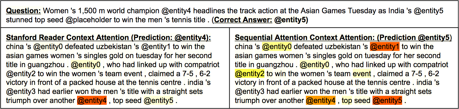
Figure 2: Representative sample output for the Stanford Reader and our model.

4.1 Results

Who did What

In our experiments the Stanford Reader (SR) achieved an accuracy of $65.6\%$ on the strict WDW dataset compared to the $64\%$ that Onishi et al. (2016) reported. The Sequential Attention model (SA) with partial-bilinear scoring function got $67.21\%$, which is the second best performance on the $WDW$ leaderboard, only surpassed by the $71.2\%$ from the Gated Attention Reader (GA) with qe-comm Li et al. (2016) features and fixed GloVe embeddings. However, the GA model without qe-comm features and fixed embeddings performs significantly worse at $67\%$. We did not use these features in our SA models, and it is likely that adding these features could further improve SA model performance. We also experimented with fixed embeddings in SA models, but fixed embeddings reduced SA performance.

Another experiment we conducted was to add $100$K training samples from CNN to the WDW data. This increase in the training data size boosted accuracy by $1.4\%$ with the SR and $1.8\%$ with the Sequential Attention model reaching a $69\%$ accuracy. This improvement strongly suggests that the gap in performance/difficulty between the CNN and the WDW datasets is partially related to the difference in the training set sizes which results in overfitting.

CNN

For a final sanity check and a fair comparison against a well known benchmark, we ran our Sequential Attention model on exactly the same CNN data used by Chen et al. (2016).

The Sequential Attention model with partial-bilinear attention scoring function took an average of 2X more time per epoch to train vs. the Stanford Reader. However, our model converged in only 17 epochs vs. 30 for the SR. The results of training the SR on CNN were slightly lower than the $73.6\%$ reported by Chen et al. (2016). The Sequential Attention model achieved $77.1\%$ accuracy, a $3.7\%$ gain with respect to SR.

4.1.1 Model comparison on CNN

After achieving good performance with SA we wanted to understand what was driving the increase in accuracy. It is clear that SA has more trainable parameters compared to SR. However, it was not clear if the additional computation required to learn those parameters should be allocated in the attention mechanism, or used to compute richer hidden representations of the passage and questions. Additionally, the bilinear parameters increase the computational requirements, but their impact on performance was not clear. To answer these questions we compared the following models: i) SR with dot-product attention; ii) SR with bilinear attention; iii) SR with two layers (to compute the hidden question and passage representations) and dot-product attention; iv) SR with two layers and bilinear attention; v) SA with elementwise multiplication scoring function; vi) SA with partial-bilinear scoring function.

Surprisingly, the element-wise version of SA performed better than the partial-bilinear version, with an accuracy of $77.3\%$ which, to our knowledge, has only been surpassed by Dhingra et al. (2016) with their Gated-Attention Reader model.

Additionally, 1-layer SR with dot-product attention got $0.3\%$ lower accuracy than the 1-layer SR with bilinear attention. These results suggest that the bilinear parameters do not significantly improve performance over dot-product attention.

Adding an additional GRU layer to encode the passage and question in the SR model increased performance over the original 1-layer model. With dot-product attention the increase was $1.1\%$ whereas with bilinear attention, the increase was $1.3\%$. However, these performance increases were considerably less than the lift from using an SA model (and SA has fewer parameters).

Model	CNN	Params
SR, dot prod. att.	73.1%	$5.44\times 10^{6}$
SR, bilinear att.	73.4%	$5.50\times 10^{6}$
SR, 2-layer, dot prod. att.	74.2%	$5.83\times 10^{6}$
SR, 2-layer, bilinear att.	74.7%	$5.90\times 10^{6}$
SA, element-wise att.	77.3%	$5.73\times 10^{6}$
SA, partial-bilinear att.	77.1%	$5.80\times 10^{6}$

Table 2: Accuracy on CNN test sets and number of trainable parameters for various Stanford Reader (SR) and Sequential Attention (SA) models.

4.2 Discussion

The difference between our Sequential Attention and standard approaches to attention is that we conserve the distributed representation of similarity for each token and use that contextual information when computing attention over other words. In other words, when the bilinear attention layer computes $\alpha_{i}=\textrm{softmax}_{i}(\boldsymbol{j}\mathbf{W}\boldsymbol{h_{i}})$, it only cares about the magnitude of the resulting $\alpha_{i}$ (the amount of attention that it gives to that word). Whereas if we keep the vector $\boldsymbol{\gamma_{i}}$ we can also know which were the dimensions of the distributed representation of the attention that weighted in that decision. Furthermore, if we use that information to feed a new GRU, it helps the model to learn how to assign attention to surrounding words.

Compared to Sequential Attention, Bidirectional attention flow uses a considerably more complex architecture with a query representations for each word in the question. Unlike the Gated Attention Reader, SA does not require intermediate soft attention and it uses only one additional RNN layer. Furthermore, in SA no dot product is required to compute attention, only the sum of the elements of the $\boldsymbol{\eta}$ vector. SA’s simpler architecture performs close to the state-of-the-art.

Figure 2 shows some sample model behavior. In this example and elsewhere, SA results in less sparse attention vectors compared to SR, and this helps the model assign attention not only to potential target strings (anonymized entities) but also to relevant contextual words that are related to those entities. This ultimately leads to richer semantic representations $\boldsymbol{o}=\sum\alpha_{i}\boldsymbol{h_{i}}$ of the passage.

Finally, we found: i) bilinear attention does not yield dramatically higher performance compared to dot-product attention; ii) bilinear parameters do not improve SA performance; iii) Increasing the number of layers in the attention mechanism yields considerably greater performance gains with fewer parameters compared to increasing the number of layers used to compute the hidden representations of the question and passage.

5 Conclusion and Discussion

In this this paper we created a novel and simple model with a Sequential Attention mechanism that performs near the state of the art on the CNN and WDW datasets by improving the bilinear and dot-product attention mechanisms with an additional bi-directional RNN layer. This additional layer allows local alignment information to be used when computing the attentional score for each token. Furthermore, it provides higher performance gains with fewer parameters compared to adding an additional layer to compute the question and passage hidden representations. For future work we would like to try other machine reading datasets such as SQuAD and MS MARCO. Also, we think that some elements of the SA model could be mixed with ideas applied in recent research from Dhingra et al. (2016) and Seo et al. (2016). We believe that the SA mechanism may benefit other tasks as well, such as machine translation.

References

- Bahdanau et al. (2014) Dzmitry Bahdanau, Kyunghyun Cho, and Yoshua Bengio. 2014. Neural machine translation by jointly learning to align and translate. CoRR abs/1409.0473. http://arxiv.org/abs/1409.0473.
- Chen et al. (2016) Danqi Chen, Jason Bolton, and Christopher D. Manning. 2016. A thorough examination of the cnn/daily mail reading comprehension task. CoRR abs/1606.02858. http://arxiv.org/abs/1606.02858.
- Cho et al. (2014) Kyunghyun Cho, Bart van Merrienboer, Çaglar Gülçehre, Fethi Bougares, Holger Schwenk, and Yoshua Bengio. 2014. Learning phrase representations using RNN encoder-decoder for statistical machine translation. CoRR abs/1406.1078. http://arxiv.org/abs/1406.1078.
- Dhingra et al. (2016) Bhuwan Dhingra, Hanxiao Liu, William W. Cohen, and Ruslan Salakhutdinov. 2016. Gated-attention readers for text comprehension. CoRR abs/1606.01549. http://arxiv.org/abs/1606.01549.
- Dieleman et al. (2015) Sander Dieleman, Jan Schlüter, Colin Raffel, Eben Olson, Søren Kaae Sønderby, Daniel Nouri, Daniel Maturana, Martin Thoma, Eric Battenberg, Jack Kelly, Jeffrey De Fauw, Michael Heilman, Diogo Moitinho de Almeida, Brian McFee, Hendrik Weideman, Gábor Takács, Peter de Rivaz, Jon Crall, Gregory Sanders, Kashif Rasul, Cong Liu, Geoffrey French, and Jonas Degrave. 2015. Lasagne: First release. https://doi.org/10.5281/zenodo.27878.
- Hermann et al. (2015) Karl Moritz Hermann, Tomás Kociský, Edward Grefenstette, Lasse Espeholt, Will Kay, Mustafa Suleyman, and Phil Blunsom. 2015. Teaching machines to read and comprehend. CoRR abs/1506.03340. http://arxiv.org/abs/1506.03340.
- Kim et al. (2017) Yoon Kim, Carl Denton, Luong Hoang, and Alexander M. Rush. 2017. Structured attention networks. CoRR abs/1702.00887. http://arxiv.org/abs/1702.00887.
- Li et al. (2016) Peng Li, Wei Li, Zhengyan He, Xuguang Wang, Ying Cao, Jie Zhou, and Wei Xu. 2016. Dataset and neural recurrent sequence labeling model for open-domain factoid question answering. CoRR abs/1607.06275. http://arxiv.org/abs/1607.06275.
- Luong et al. (2015) Minh-Thang Luong, Hieu Pham, and Christopher D. Manning. 2015. Effective approaches to attention-based neural machine translation. CoRR abs/1508.04025. http://arxiv.org/abs/1508.04025.
- Onishi et al. (2016) Takeshi Onishi, Hai Wang, Mohit Bansal, Kevin Gimpel, and David A. McAllester. 2016. Who did what: A large-scale person-centered cloze dataset. CoRR abs/1608.05457. http://arxiv.org/abs/1608.05457.
- Pennington et al. (2014) Jeffrey Pennington, Richard Socher, and Christopher D. Manning. 2014. Glove: Global vectors for word representation. In Empirical Methods in Natural Language Processing (EMNLP). pages 1532–1543. http://www.aclweb.org/anthology/D14-1162.
- Seo et al. (2016) Min Joon Seo, Aniruddha Kembhavi, Ali Farhadi, and Hannaneh Hajishirzi. 2016. Bidirectional attention flow for machine comprehension. CoRR abs/1611.01603. http://arxiv.org/abs/1611.01603.
- Theano Development Team (2016) Theano Development Team. 2016. Theano: A python framework for fast computation of mathematical expressions. CoRR abs/1605.02688. http://arxiv.org/abs/1605.02688.