Coherent quadrupole-octupole states from a SUSY-QM Hamiltonian hierarchy and shape invariance

Coherent quadrupole-octupole states from a SUSY-QM Hamiltonian hierarchy …N. Minkov, S. Drenska, P. Yotov

, S. Drenska , P. Yotov

We show that the potential in the radial equation in the model of coherent quadrupole-octupole motion (CQOM) in nuclei generates a sequence of superpotentials and subsequent series of effective potentials which satisfy the shape-invariance condition and correspond to a SUSY-QM hierarchy of Hamiltonians. On this basis we suggest that the original CQOM level scheme possesses a generic supersymmetric structure of the spectrum inherent for the coherent quadrupole-octupole mode. We outline the mechanism in which the real quadrupole-octupole spectra in even-even and odd-even nuclei deviate from the genuine symmetry. By using it we illustrate the possibilities to identify the signs of supersymmetry in the alternating-parity spectra of even-even nuclei and the quasi-parity-doublet levels of odd-mass nuclei described within the CQOM model approach.

1 Introduction

The supersymmetry (SUSY) concept in physics was introduced as a part of the efforts for a unified description of the basic interactions in nature [1]. Within SUSY one may consider the fundamental particles – fermions and bosons – as superpartners related by a transformation which keeps the same mass and changes the spin by 1/2. Since the masses of the presently observed particles do not allow one to identify any pair of superpartners, it appears that the genuine SUSY does not exist at the currently accessible energies, whereas a spontaneous symmetry breaking mechanism providing different masses for the superpartners may take a place [2]. Nevertheless, the specific algebraic structure of SUSY, which includes a combination of commutation (bosonic) and anti-commutation (fermionic) relations, can be associated in a more general context with the solution of some quantum mechanical problems and has lead to the development of the so-called supersymmetric quantum mechanics (SUSY-QM) [3, 4]. In particular, it was realized [5] that the SUSY-QM leads to a deeper understanding of the factorization approaches [6, 7] applied in the solution of the Schrödinger equation and allows one to outline and properly systematize the various classes of known analytically solvable potentials. A common feature of all these potentials, hereafter called SUSY potentials, is that each of them generates a hierarchy of factorized Hamiltonians the eigenvalues of which exhaust the spectrum of the given potential. Also, it is known that some SUSY potentials satisfy the so-called shape invariance condition [8]. In this case all potentials in the hierarchy have the same functional dependence on the (space) variable and only differ through a set of discrete parameters which change under given rule at the subsequent hierarchy steps. The different potentials are related through certain recurrence relation allowing one to obtain simplified expressions for the energies and wave functions in the spectrum. A classification of some basic shape invariant potentials (SIPs) is given in [9].

The SUSY-QM formalism was extended to Hamiltonians with coordinate-dependent effective mass [10, 11]. The shape-invariance condition was generalized (deformed) for the respectively obtained effective potentials allowing one to apply the SUSY-QM techniques for solving the eigenvalue problem. Recently this concept was applied to nuclear collective models [12, 13, 14]. The SUSY-QM technique for SIPs was applied to solve the eigenvalue problem for Bohr-like Hamiltonians with deformation-dependent mass terms in the cases of Davidson [12, 13] and Kratzer [14] potentials. The approach allows one to obtain analytical expressions for spectra and wave functions for separable potentials in the cases of axially-symmetric prolate deformed nuclei, $\gamma$-unstable nuclei and triaxial nuclei. The dependence of the mass on the deformation moderates the increase of the moment of inertia with deformation, removing a known drawback of the Bohr model. As a result a good description of ground-, $\beta$-, $\gamma$- energy band levels and the attendant B(E2) transition probabilities in a wide range of nuclei in different regions of collectivity was obtained with a reasonable accuracy.

Another collective model assuming a coherent quadrupole-octupole motion (CQOM) in nuclei was developed by using a two-dimensional potential depending on the axial quadrupole and octupole deformation variables [15]–[18]. The assumption of coherence allows one to exactly separate the variables in ellipsoidal coordinates obtaining a “radial” equation for the effective quadrupole-octupole deformation and “angular” equation for the relative quadrupole-octupole excitation modes. The radial equation involves a Davidson-like potential which allows one to find an analytical solution of the model. The obtained spectrum corresponds to coherent quadrupole-octupole vibrations coupled to rotation motions of the nucleus. It was shown that the model is capable to describe and classify the yrast and higher excited alternating-parity sequences in even-even nuclei and split parity-doublet spectra in odd-mass nuclei. The analytical solvability and classification ability of the model make it interesting to examine the possibly underlying symmetry which determines the properties of the model system as well as to check to what extent such a symmetry can be identified in the observed experimental spectra.

The aim of the present work is to clarify the above issue by applying the SUSY-QM techniques to the CQOM model Hamiltonian. It will be shown that the potential in the radial equation is shape invariant and this allows one to express the Hamiltonian in terms of the SUSY hierarchy and to subsequently obtain the model spectrum through the SUSY-QM procedure. We shall examine the possibility to associate SUSY with the coherent quadrupole-octupole modes assumed in the model. At the same time we shall study the deviation of the experimentally observed quadrupole-octupole spectra from the model imposed scheme. This should allow us to look for a proper symmetry-breaking mechanism which may govern the observed collective properties of nuclei.

In Sec. 2 an overview of the SUSY-QM and SIP concepts is given by using the formulations provided in [5]. In Sec. 3 the application of the SUSY-QM techniques to the CQOM model is presented. In Sec. 4 the possibility to associate CQOM with SUSY is considered together with the analysis of observed spectra and related discussion. In Sec. 5 concluding remarks are given.

2 SUSY-QM formalism for analytically solvable potentials

2.1 Supersymmetric factorization of a solvable one-dimensional Hamiltonian

Let us consider the ground-state (gs) wave function $\psi_{0}(x)$ and energy $E_{0}$ for a one-dimensional potential $V(x)$ which satisfy the Schrödinger equation

$$H\psi_{0}(x)=-\frac{\hbar^{2}}{2m}\frac{d^{2}\psi_{0}(x)}{dx^{2}}+V(x)\psi_{0}(x)=E_{0}\psi_{0}(x).$$ (1)

If $\psi_{0}(x)$ is nodeless and the potential $V(x)\rightarrow V_{-}(x)=V(x)-E_{0}$ is shifted so as $E_{0}\rightarrow E^{-}_{0}=0$, with $\psi_{0}^{-}(x)\equiv\psi_{0}(x)$, one obtains from (1)

$$V_{-}(x)=\frac{\hbar^{2}}{2m}\frac{\psi_{0}^{{}^{\prime\prime}-}(x)}{\psi_{0}^{-}(x)}\ ,$$ (2)

and $H\rightarrow H_{-}$ such that

$$H_{-}\psi_{0}^{-}(x)=-\frac{\hbar^{2}}{2m}\frac{d^{2}\psi_{0}^{-}(x)}{dx^{2}}+V_{-}(x)\psi_{0}^{-}(x)=0.$$ (3)

If the function $\psi_{0}^{-}(x)$ is known or guessed the potential $V_{-}(x)$ can be determined from (2) up to a constant. Hamiltonian (3) can be factorized in the form [5]

$$H_{-}=A^{{\dagger}}A.$$ (4)

The operators $A$ and $A^{{\dagger}}$ are defined as first order differential operators

$$A=\frac{\hbar}{\sqrt{2m}}\frac{d}{dx}+W(x),\ \ A^{{\dagger}}=-\frac{\hbar}{\sqrt{2m}}\frac{d}{dx}+W(x),$$ (5)

where the unknown function $W(x)$ is determined so that Eq. (3) is satisfied after introducing (4) and (5)

$$H_{-}\psi_{0}^{-}(x)=\left[-\frac{h^{2}}{2m}\frac{d^{2}}{dx^{2}}-\frac{h}{\sqrt{2m}}W^{\prime}(x)+W^{2}(x)\right]\psi_{0}^{-}(x)=0.$$ (6)

By comparing Eqs. (6) and (3) one finds:

$$V_{-}(x)=W^{2}(x)-\frac{\hbar}{\sqrt{2m}}W^{\prime}(x).$$ (7)

This equation is a first order differential equation for the function $W(x)$ known as Riccati equation [19]. By taking $V_{-}(x)$ from (2) its solution is obtained as [5]

$$W(x)=-\frac{\hbar}{\sqrt{2m}}\frac{\psi_{0}^{{}^{\prime}-}(x)}{\psi_{0}^{-}(x)}=-\frac{\hbar}{\sqrt{2m}}\frac{d}{dx}\ln[\psi_{0}^{-}(x)].$$ (8)

Then the action of $A$ on the gs wave function gives

$$A\psi_{0}^{-}(x)=\frac{\hbar}{\sqrt{2m}}\frac{d}{dx}\psi_{0}^{-}(x)+W(x)\psi_{0}^{-}(x)=0,$$ (9)

which allows one to determine $\psi_{0}^{-}(x)$ by $W(x)$

$$\psi_{0}^{-}(x)=N\exp\left(-\frac{\sqrt{2m}}{\hbar}\int^{x}W(k)dk\right)\ ,$$ (10)

where $N$ is a normalization constant.

By changing the order of the operators in the factorization (4) one defines a new Hamiltonian

$$H_{+}=AA^{{\dagger}},$$ (11)

whose action on the gs wave function

$$H_{+}\psi_{0}^{-}(x)=\left[-\frac{h^{2}}{2m}\frac{d^{2}}{dx^{2}}+\frac{h}{\sqrt{2m}}W^{\prime}(x)+W^{2}(x)\right]\psi_{0}^{-}(x)$$ (12)

defines a new potential [5]

$$V_{+}(x)=W^{2}(x)+\frac{\hbar}{\sqrt{2m}}W^{\prime}(x)$$ (13)

related to $V_{-}(x)$, $W(x)$ and $W^{\prime}(x)$ through

$$\frac{1}{2}[V_{-}(x)+V_{+}(x)]=W^{2}(x),\ \ \frac{1}{2}[V_{-}(x)-V_{+}(x)]=W^{\prime}(x)\ .$$ (14)

Also, one has

$$[A,A^{{\dagger}}]=\frac{-2\hbar}{\sqrt{2m}}W^{\prime}(x).$$ (15)

The function $W(x)$ is known as superpotential, while the potentials $V_{-}(x)$ and $V_{+}(x)$ are called supersymmetric partners.

By considering the eigenfunctions $\psi_{n}^{-}(x)$, $\psi_{n}^{+}(x)$ and eigenvalues $E_{n}^{-}$, $E_{n}^{+}$ ($n=0,1,2\dots$) of the Hamiltonians $H_{-}$ and $H_{+}$, respectively, one can easily check that $H_{+}(A\psi_{n}^{-}(x))=E_{n}^{-}(A\psi_{n}^{-}(x))$ and $H_{-}(A^{{\dagger}}\psi_{n}^{+}(x))=E_{n}^{+}(A^{{\dagger}}\psi_{n}^{+}(x))$ which together with (9) leads to the relations

$$E_{n}^{+} = E_{n+1}^{-}\ ,\ \ \ \mbox{with }\ E_{0}^{-}=0$$ (16)

$$\psi_{n}^{+}(x) = \left(E_{n+1}^{-}\right)^{-\frac{1}{2}}A\psi_{n+1}^{-}(x)\ ,\ \ \ \psi_{n+1}^{-}(x)=\left(E_{n}^{+}\right)^{-\frac{1}{2}}A^{{\dagger}}\psi_{n}^{+}(x).$$ (17)

It is seen that the spectra of $H_{-}$ and $H_{+}$ are identical except for $E_{0}^{-}$ which does not appear for $H_{+}$. By using (17) one can obtain the eigenfunctions of $H_{-}$ from those of $H_{+}$ and vice versa, except for $\psi_{0}^{-}$ which is determined by the superpotential in (10). $H_{-}$ and $H_{+}$ are referred to as SUSY partners. Together with the operators $A$ and $A^{{\dagger}}$ they form a set of matrices [5]

$$H=\left(\begin{array}[]{cc}H_{-}&0\\ 0&H_{+}\\ \end{array}\right)\ \ \ \ \ Q=\left(\begin{array}[]{cc}0&0\\ A&0\\ \end{array}\right)\ \ \ \ \ Q^{+}=\left(\begin{array}[]{cc}0&A^{{\dagger}}\\ 0&0\\ \end{array}\right),$$

which satisfy the following commutation and anti-commutation relations

$$[H,Q]=[H,Q^{+}]=0,\ \ \ \{Q,Q^{+}\}=H,\ \ \ \{Q^{+},Q^{+}\}=\{Q,Q\}=0$$ (18)

closing the superalgebra of $sl(1,1)$. The operators $Q$ and $Q^{+}$ are known in the SUSY theory as supercharges and can be interpreted as operators transforming the bosonic degrees of freedom into fermionic ones. The fact that they commute with $H$ is related to the supersymmetric degeneracy of the spectrum. The SUSY algebra is an extension of the Poincare algebra [3, 5].

2.2 SUSY-QM hierarchy of Hamiltonians and shape invariant potentials

Starting by $H^{(1)}\equiv H_{-}$ and $H^{(2)}\equiv H_{+}$, Eqs. (4) and (11), a hierarchy of supersymmetric partner Hamiltonians $H^{(1)},\ H^{(2)},H^{(3)},\dots$ can be constructed, so that $H^{(3)}$ is obtained as the upper superpartner of $H^{(2)}$ after factorizing the latter by analogy to $H^{(1)}$, $H^{(4)}$ is constructed by $H^{(3)}$ in the same way, and so on. In this procedure the levels of each subsequent Hamiltonian are obtained from the previous one by removing its lowest level. Thus, knowing the eigenvalues and eigenfunctions of $H^{(1)}$ one obtains the eigenvalues and eigenfunctions of all Hamiltonians in the hierarchy. The energy levels appearing in the hierarchy are illustrated schematically below.

$$\begin{aligned} E_{5}^{(1)}\frac{\hskip 14.22636pt}{\hskip 14.22636pt}&\;&E_{4}^{(2)}\frac{\hskip 14.22636pt}{\hskip 14.22636pt}&\;&E_{3}^{(3)}\frac{\hskip 14.22636pt}{\hskip 14.22636pt}&\;&E_{2}^{(4)}\frac{\hskip 14.22636pt}{\hskip 14.22636pt}&\;&E_{1}^{(5)}\frac{\hskip 14.22636pt}{\hskip 14.22636pt}&\;&E_{0}^{(6)}\frac{\hskip 14.22636pt}{\hskip 14.22636pt}&\;\\ E_{4}^{(1)}\frac{\hskip 14.22636pt}{\hskip 14.22636pt}&\;&E_{3}^{(2)}\frac{\hskip 14.22636pt}{\hskip 14.22636pt}&\;&E_{2}^{(3)}\frac{\hskip 14.22636pt}{\hskip 14.22636pt}&\;&E_{1}^{(4)}\frac{\hskip 14.22636pt}{\hskip 14.22636pt}&\;&E_{0}^{(5)}\frac{\hskip 14.22636pt}{\hskip 14.22636pt}&\;\\ E_{3}^{(1)}\frac{\hskip 14.22636pt}{\hskip 14.22636pt}&\;&E_{2}^{(2)}\frac{\hskip 14.22636pt}{\hskip 14.22636pt}&\;&E_{1}^{(3)}\frac{\hskip 14.22636pt}{\hskip 14.22636pt}&\;&E_{0}^{(4)}\frac{\hskip 14.22636pt}{\hskip 14.22636pt}&\;\\ E_{2}^{(1)}\frac{\hskip 14.22636pt}{\hskip 14.22636pt}&\;&E_{1}^{(2)}\frac{\hskip 14.22636pt}{\hskip 14.22636pt}&\;&E_{0}^{(3)}\frac{\hskip 14.22636pt}{\hskip 14.22636pt}&\;\\ E_{1}^{(1)}\frac{\hskip 14.22636pt}{\hskip 14.22636pt}&\;&E_{0}^{(2)}\frac{\hskip 14.22636pt}{\hskip 14.22636pt}&\;\\ E_{0}^{(1)}\frac{\hskip 14.22636pt}{\hskip 14.22636pt}&\;\\ H^{(1)}&&H^{(2)}&&H^{(3)}&&H^{(4)}&&H^{(5)}&&H^{(6)}\end{aligned}$$

The pair of supersymmetric partner potentials $V_{\pm}(x)$ defined by (7) and (13) represents a shape invariant if they satisfy the condition[8]

$$V_{+}(x;a_{1})=V_{-}(x;a_{2})+R(a_{1}),$$ (19)

where $a_{1}$ is a set of parameters, while $a_{2}=f(a_{1})$ and $R(a_{1})$ are functions of $a_{1}$ but not of $x$. In this case all supersymmetric partner potentials appearing in the hierarchy of Hamiltonians can be simply expressed in the form of $V_{-}$, so that

$$H^{(1)} =-\frac{h^{2}}{2m}\frac{d^{2}}{dx^{2}}+V_{-}(x;a_{1})$$

$$H^{(2)} =-\frac{h^{2}}{2m}\frac{d^{2}}{dx^{2}}+V_{-}(x;a_{2})+R(a_{1})$$

$$... ..........................................$$

$$H^{(m)} \equiv-\frac{h^{2}}{2m}\frac{d^{2}}{dx^{2}}+V_{-}(x;a_{m})+\sum_{k=1}^{m-1}R(a_{k}),$$

where $a_{m}=f^{(m-1)}(a_{1})$. The gs energies of the different Hamiltonians are

$$E_{0}^{(m)}=\sum_{k=1}^{m-1}R(a_{k})+E_{0}^{(1)}.$$ (20)

The complete energy spectrum of $H^{(1)}$ is

$$E_{n}^{(1)}=\sum_{k=1}^{n}R(a_{k}),\ \mbox{with}\ E_{0}^{(1)}=0,\ n=0,1,2,...$$ (21)

while the corresponding eigenfunctions are determined by

$$\psi_{n}^{(1)}(x;a_{1})\backsim A^{{\dagger}}(x;a_{1})A^{{\dagger}}(x;a_{2})...A^{{\dagger}}(x;a_{n})\psi_{0}^{(1)}(x;a_{n+1}),$$ (22)

where the operators $A^{{\dagger}}(x;a_{n})$ are determined by (5) with $W(x;a_{n})$ being a function of $V_{-}(x;a_{n})$ and $\sum_{k=1}^{n-1}R(a_{k})$.

3 SUSY-QM formalism in the CQOM model

3.1 The problem of soft quadrupole-octupole vibrations and rotations

The Hamiltonian of quadrupole-octupole vibrations and rotations has been taken in the form [15]–[18]

$$H_{\mbox{\scriptsize qo}} = -\frac{\hbar^{2}}{2B_{2}}\frac{\partial^{2}}{\partial\beta_{2}^{2}}-\frac{\hbar^{2}}{2B_{3}}\frac{\partial^{2}}{\partial\beta_{3}^{2}}+U(\beta_{2},\beta_{3},I),$$ (23)

where $\beta_{2}$ and $\beta_{3}$ are axial quadrupole and octupole variables and the potential is

$$U(\beta_{2},\beta_{3},I)=\frac{1}{2}C_{2}{\beta_{2}}^{2}+\frac{1}{2}C_{3}{\beta_{3}}^{2}+\frac{X(I)}{d_{2}\beta_{2}^{2}+d_{3}\beta_{3}^{2}}.$$ (24)

Here $B_{2}$ $(B_{3})$, $C_{2}$ $(C_{3})$ and $d_{2}$ ($d_{3}$) are quadrupole (octupole) mass, stiffness and inertia parameters, respectively, and $X(I)$ involves the angular momentum dependence of the spectrum specified in [15, 16]. Under the assumption of coherent quadrupole-octupole oscillations with a frequency $\omega=\sqrt{C_{2}/B_{2}}=\sqrt{C_{3}/B_{3}}\equiv\sqrt{C/B}$ and by introducing ellipsoidal coordinates $\beta_{2}=\sqrt{d/d_{2}}\eta$ $\cos\phi$, $\beta_{3}=\sqrt{d/d_{3}}\eta\sin\phi$, with $d=(d_{2}+d_{3})/2$, one obtains the Schrödinger equation for (23) with separated variables

$$\frac{d^{2}\psi(\eta)}{d\eta^{2}}+\frac{1}{\eta}\frac{d\psi}{d\eta}+\frac{2B}{\hbar^{2}}\left[E-\frac{\hbar^{2}}{2B}\frac{k^{2}}{\eta^{2}}-\frac{1}{2}C\eta^{2}-\frac{X(I)}{d\eta^{2}}\right]\psi(\eta)=0$$ (25)

$$\frac{\partial^{2}}{\partial\phi^{2}}\varphi(\phi)+k^{2}\varphi(\phi)=0\ .$$ (26)

By substituting

$$\psi(\eta)=\eta^{-1/2}\varphi(\eta)$$ (27)

the radial equation is obtained in the form

$$\frac{d^{2}\varphi(\eta)}{d\eta^{2}}+\frac{2B}{\hbar^{2}}\left[E-\frac{\hbar^{2}}{2B}\frac{k^{2}}{\eta^{2}}-\frac{1}{2}C\eta^{2}-\frac{X(I)}{d\eta^{2}}+\frac{1}{4}\frac{\hbar^{2}}{2B\eta^{2}}\right]\varphi(\eta)=0.$$ (28)

3.2 Shape invariance of the CQOM potential

Applying the SUSY-QM procedure to Eq. (28), we consider the effective potential in the ground state ($E=E_{0}$) as the first (lowest) superpartner potential

$$V_{-}(\eta)=V_{\mbox{\scriptsize eff}}=\frac{1}{2}B\omega^{2}\eta^{2}+\frac{\hbar^{2}}{2B\eta^{2}}\left(s^{2}-\frac{1}{4}\right)-E_{0},$$ (29)

where $s=s(k,I)=\sqrt{k^{2}+bX(I)}$, with $b=2B/\hbar^{2}d$. (Note that in Refs. [15]–[18] the quantity $s$ includes an additional factor 1/2 ). To find the SUSY partner potential $V_{+}$, Eq. (13), the Riccati equation (7) for the superpotential $W(\eta)$ has to be solved. We search $W(\eta)$ in the form

$$W(\eta)=a_{1}\eta-\frac{a_{2}}{\eta},$$ (30)

where $a_{1}$ and $a_{2}$ are parameters to be determined. By substituting (29) and (30) into the left and right hand sides of (7), respectively, and after equating the powers of $\eta$ in both sides one finds

$$a_{1}=\omega\sqrt{\frac{B}{2}},\ \ \ a_{2}=\frac{\hbar}{\sqrt{2B}}(s+1/2),\ \ \ E_{0}(s)=\hbar\omega(1+s)\ .$$ (31)

As a result the superpotential $W(\eta)$ becomes

$$W(\eta)=W(\eta,s)=\sqrt{\frac{B}{2}}\omega\eta-\frac{\hbar}{\sqrt{2B}}\frac{(s+1/2)}{\eta}\ ,$$ (32)

and the potentials $V_{-}(\eta,s)$ and $V_{+}(\eta,s)$ which now determine the partner Hamiltonians $H^{(1)}$ and $H^{(2)}$ are obtained in the form

$$V_{-}(\eta;s) = \frac{1}{2}B\omega^{2}\eta^{2}+\frac{\hbar^{2}}{2B\eta^{2}}(s-1/2)(s+1/2)-\hbar\omega(s+1)$$ (33)

$$V_{+}(\eta;s) = \frac{1}{2}B\omega^{2}\eta^{2}+\frac{\hbar^{2}}{2B\eta^{2}}(s+1/2)(s+3/2)-\hbar\omega s\ .$$ (34)

It is easily seen that $V_{-}$ and $V_{+}$ satisfy the shape invariance condition Eq. (19) with $R(s)=R=2\hbar\omega$ not depending on $s$.

3.3 SUSY-QM hierarchy and solution of the CQOM eigenproblem

By continuing the above procedure one gets the SUSY-CQOM potential partners in the following general form

$$V_{-}(\eta;s+m-1) = \frac{1}{2}B\omega^{2}\eta^{2}+\frac{\hbar^{2}}{2B\eta^{2}}(s-\frac{1}{2}+m-1)(s+\frac{1}{2}+m-1)$$

$$+ 2(m-1)\hbar\omega,$$

$$V_{-}(\eta;s+m) = \frac{1}{2}B\omega^{2}\eta^{2}+\frac{\hbar^{2}}{2B\eta^{2}}(s-\frac{1}{2}+m)(s+\frac{1}{2}+m)$$

$$+ 2m\hbar\omega.$$

As a result the SUSY-hierarchy Hamiltonians and their ground-state energies are obtained in the following schematic form

$H^{(1)}\rightarrow V_{-}(s)+E_{0}(s)\rightarrow E_{0}^{(1)}(s)$

$H^{(2)}\rightarrow V_{-}(s+1)+2\hbar\omega+E_{0}(s)\rightarrow E_{0}^{(2)}(s)=E_{1}^{(1)}(s)$

$H^{(3)}\rightarrow V_{-}(s+2)+4\hbar\omega+E_{0}(s)\rightarrow E_{0}^{(3)}(s)=E_{2}^{(1)}(s)$

……………………………………………………………………..

$H^{(m)}\rightarrow V_{-}(s+m-1)+2(m-1)\hbar\omega+E_{0}(s)\rightarrow E_{0}^{(m)}(s)=E_{m-1}^{(1)}(s)$

$H^{(m+1)}\rightarrow V_{-}(s+m)+2m\hbar\omega+E_{0}(s)\rightarrow E_{0}^{(m+1)}(s)=E_{m}^{(1)}(s)$ .

According to (21) the energies $E_{n}(s)\equiv E_{n}^{(1)}(s)$, $n=0,1,2,\dots$ form the full spectrum of $H^{(1)}$ which enters the radial CQOM equation (28). Thus one obtains the CQOM spectrum given in [15]

$$E_{n}(s)=E_{nk}(I)=\hbar\omega\left[2n+s(k,I)+1\right]=\hbar\omega\left[2n+1+\sqrt{k^{2}+bX(I)}\right].$$ (35)

The ground state wave function for $H^{(1)}$, with $n=0$, is obtained by introducing $W(\eta,s)$, Eq (32), into Eq. (10)

$$f_{0}(\eta,s) = N_{0}\exp\left[-\frac{\sqrt{2B}}{\hbar}\int^{\eta}\left(\sqrt{\frac{B}{2}}\omega x-\frac{\hbar}{\sqrt{2B}}\frac{(s+1/2)}{x}\right)dx\right]$$ (36)

$$= N_{0}\,\exp\left(-\frac{c\eta^{2}}{2}\right)\eta^{(s+1/2)},\hskip 8.5359pt$$

where $c=\sqrt{BC}/\hbar$ and the normalization factor is $N_{0}=\sqrt{\frac{2c^{s+1}}{\Gamma(s+1)}}$. Further, by applying the general expression (22) for the next state ($n=1$) one finds

$$f_{1}(\eta,s) = N_{1}A^{{\dagger}}(\eta,s)f_{0}(\eta,s+1)$$ (37)

$$= N_{1}(-c\eta^{2}+s+1)\exp\left(-\frac{c\eta^{2}}{2}\right)\eta^{(s+1/2)}\ ,$$

with $N_{1}=\sqrt{\frac{2c^{s+1}}{\Gamma(s+2)}}$. By continuing this procedure, one finds by induction the known radial wave function of CQOM [17]

$$f_{n}(\eta,s)=\psi^{I}_{n,k}(\eta)=\sqrt{\frac{2c\Gamma(n+1)}{\Gamma(n+2s+1)}}e^{-c\eta^{2}/2}(c\eta^{2})^{s}L^{2s}_{n}(c\eta^{2})\ ,$$ (38)

which involves the generalized Laguerre polynomials in the variable $\eta$.

4 The meaning of SUSY and its breaking in CQOM: Discussion

The quadrupole-octupole vibration spectrum obtained by the analytic expression (35) is schematically illustrated in Fig. 1. It consists of $k=1,2,3\dots$ level-sequences built on different $n=0,1,2,\dots$ excitations. In addition, on each $k$-level a rotation band (not given for simplicity) is built, with the allowed angular momentum values depending on parity conditions imposed by the model (see below). The different $n$-sequences have identical structures and are equally shifted by $2\hbar\omega$. It is seen that the bandheads $(n=0,1,2,\dots,k=1,I=I_{\mbox{\scriptsize bh}})$ of these sequences generate the full SUSY hierarchy of levels (given in Fig. 1 in blue) which appear in the CQOM scheme. Here $I_{\mbox{\scriptsize bh}}$ is the lowest possible (bandhead) angular momentum for given $n$, which is $0$ for the even-even nuclei and $1/2$ for odd-mass nuclei. The set of bandhead levels $E_{n,k=1}(I_{\mbox{\scriptsize bh}})$ determines the SUSY-QM content of the CQOM model. It suggests that the assumed coherent quadrupole-octupole motion in nuclei possesses a genuine SUSY inherent for the radial ($\eta$) vibration mode. At the same time the development of the $k$-sequences (i.e. the angular ($\phi$) mode) and the further superposed rotation levels can be interpreted as the result of a dynamical breaking of SUSY in which the full spectrum of the system is generated. In the present context the term “dynamical” means that the symmetry breaking is due to the involvement of additional dynamic modes (angular vibrations and rotations) represented by the quantum numbers $k$ and $I$ outside of the one-dimensional radial motion.

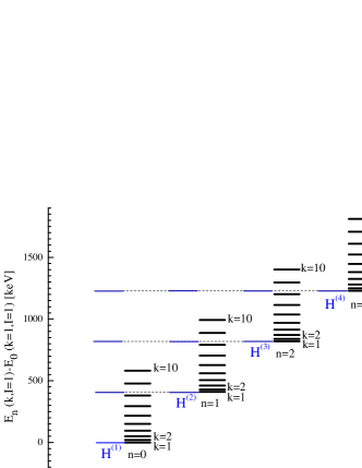
Figure 1: Schematic quadrupole-octupole vibration levels (without rotations) and SUSY-QM hierarchy (in blue) of the bandhead states in the CQOM model.

Further, by applying the model scheme to the quadrupole-octupole spectra one imposes geometrically motivated parity conditions. In the alternating-parity bands of even-even nuclei the positive-parity states correspond to an odd $k$-value, while the negative-parity states correspond to even $k$ [15, 17]. In the quasi-parity-doublets of odd-mass nuclei this correspondence depends on the odd-particle parity [16, 18]. The difference in the two $k$-values generates the parity-shift effect. This is illustrated for the alternating-parity bands in Fig. 2 by taking the lowest possible values $k=1$ and $2$. The magnitude of the parity shift can be adjusted by changing the parameters values (especially $b$ and/or $\omega$), as seen by comparing the spectra in the upper and lower parts of Fig. 2. (The shift is indicated by blue double-arrows). However, if the parity-shift differs for the different sequences in given spectrum, one needs to consider different pairs of $k$-values, like $(1,2)$, $(1,4)$, $(1,6)$ as shown in Fig. 2 or others (as e.g. in [17]), in order to reproduce the observed energy displacements. This means that a deeper mechanism of symmetry breaking may take place when the CQOM model scheme is applied to reproduce the realistic quadrupole-octupole spectra.

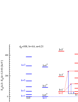
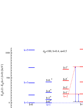
Figure 2: Schematic structure of alternating-parity spectrum in CQOM with small (upper part) and large (lower part) parity shift. The energy levels are obtained by (35) with $X(I)=[d_{0}+I(I+1)]/2$, where $d_{0}$ is a parameter of the potential.

Now we are able to examine to what extent the so-defined broken SUSY manifests in the experimental spectra of nuclei with quadrupole-octupole degrees of freedom. We can say that if these spectra possess it as a generic symmetry one should observe different sets of (almost) identical band-structures – alternating-parity bands in even-even nuclei and quasi-parity-doublets in odd-mass nuclei – shifted one from another by (almost) the same energy intervals. Indeed by looking into data one finds several examples where such structure of the spectrum can be identified. Good examples are observed for the nuclei ¹⁵²Sm, ¹⁵⁴Gd and ¹⁰⁰Mo whose CQOM-theoretical and experimental spectra are given in Figs. 1, 3 and 7, respectively of Ref. [17]. In the three nuclei it is seen that the structures of the yrast and non-yrast alternating-parity sequences are very similar and in addition in ¹⁵⁴Gd the spacing between the three $0^{+}$ bandheads is almost the same. Reasonable examples in odd-mass nuclei are the spectra of ²²³Ra (Fig. 2 in Ref. [18]) and ²³⁷U (Fig. 4 in Ref. [20]).

From another side a wider look on experimental data shows the presence of quadrupole-octupole spectra in which the different energy sequences are neither quite identical nor really equidistantly displaced. Such are the spectra in ¹⁵⁴Sm, ¹⁵⁶Gd, ¹⁵⁸Gd and ²³⁶U (Figs. 2, 4, 5 and 6 in Ref. [17]) as well as ¹⁶¹Dy and ²³⁹Pu (Figs. 2 and 4 in Ref. [21]). In these cases, especially in even-even nuclei, the different band structures (including parity-shifts) are reproduced by the model through introducing quite different pairs of $k$-values, whereas the energy displacements are reproduced by taking the lowest $k$ larger than 1. We should remark that in odd-mass nuclei the symmetry is additionally violated by the odd nucleon which not only affects the even-even core through the parity and Coriolis effects, but also may add a quasiparticle excitation energy to the doublet bandheads.

5 Conclusion

We have shown that the CQOM formalism, in which the potential is a shape invariant in the space of the effective quadrupole-octupole deformation, can be interpret in terms of the SUSY-QM approach. As a result the radial quadrupole-octupole vibrations of the nucleus are associated with a SUSY hierarchy of Hamiltonians, which together with the angular and rotation modes provide the full model spectrum of the system. This suggests that a nucleus capable of performing coherent quadrupole-octupole motions may posses a genuine SUSY, which determines the basic structure of its collective excitation spectrum. The considered examples show that if present in quadrupole-octupole spectra, the SUSY should be necessarily and multilaterally broken in dependence on various conditions and particular structure effects inherent for the even-even and odd-mass nuclei. Nevertheless, the application of the SUSY-QM concept to the CQOM model approach allows one to get a deeper insight into the symmetry properties of complex deformed nuclei as well as to better understand (and justify) the proposed model classification of nuclear quadrupole-octupole excitations. This result supports the relevance of the model scheme in nuclear quadrupole-octupole spectra and its applicability as a basis to solve the more general problem of quadrupole-octupole motions beyond the restrictions imposed by the coherent mode.

References

- [1] Y.A. Gol’fand and E.P. Likhtam, JETP Lett. 13 (1971) 323; R. Ramond, Phys. Rev. D 3 (1971) 323; D.V. Volkov and V.P. Akulov, Phys. Lett. B 46 (1973) 109; J. Wess and B. Zumino, Nucl. Phys. B 70 (1974) 39.
- [2] P. Fayet and J. Iliopoulos, Phys. Lett. B 51 (1974) 461; P. Fayet, Phys. Lett. B 58 (1975) 67.
- [3] E. Witten, Nucl. Phys. B 188 (1981) 513.
- [4] F. Cooper and B. Freedman, Ann. Phys. 146 (1983) 262.
- [5] F. Cooper, A. Khare and U. Sukhatme, Phys. Rep. 251, (1995) 267; F. Cooper, A. Khare and U. Sukhatme, Supersymmetry in Quantum Mechanics (World Scientific, Singapore, 2001).
- [6] E. Schrödinger, Proc. Roy. Irish Acad. A 46 (1940) 9.
- [7] L. Infeld and T.E. Hill, Rev. Mod. Phys. 23 (1951) 21.
- [8] L.E. Gendenshtein, Pis’ma Zh. Exp. Teor. Fiz. 38 (1983) 299; JETP Lett. 38 (1983) 356.
- [9] R. Dutt, A. Khare and U. Sukhatme, Am. J. Phys. 56 (1988) 163.
- [10] C. Quesne and V.M. Tkachuk, J. Phys. A: Math. Gen. 37 (2004) 4267.
- [11] B. Bagchi, A. Banerjee, C. Quesne and V.M. Tkachuk, J. Phys. A: Math. Gen. bf 38 (2005) 2929.
- [12] D. Bonatsos, P. Georgoudis, D. Lenis, N. Minkov and C. Quesne, Phys. Lett. B 683 (2010) 264.
- [13] D. Bonatsos, P. Georgoudis, D. Lenis, N. Minkov and C. Quesne, Phys. Rev. C 83 (2011) 044321.
- [14] D. Bonatsos, P. Georgoudis, D. Lenis, N. Minkov and C. Quesne, Phys. Rev. C 88 (2013) 034316.
- [15] N. Minkov, P. Yotov, S. Drenska, W. Scheid, D. Bonatsos, D. Lenis and D. Petrellis, Phys. Rev. C 73 (2006) 044315.
- [16] N. Minkov, S. Drenska, P. Yotov, S. Lalkovski, D. Bonatsos and W. Scheid, Phys. Rev. C 76 (2007) 034324.
- [17] N. Minkov, S. Drenska, M. Strecker, W. Scheid and H. Lenske, Phys. Rev. C 85 (2012) 034306.
- [18] N. Minkov, S. Drenska, K. Drumev, M. Strecker, H. Lenske and W. Scheid, Phys. Rev. C 88 (2013) 064310.
- [19] J. Riccati, Opere, Treviso (1758).
- [20] N. Minkov, S. Drenska, K. Drumev, M. Strecker, H. Lenske and W. Scheid, Proc. Int. Conf. “Nuclear Structure and Related Topics” (NSRT-12), Dubna, Russia, 2012, EPJ Web of Conferences 38 (2012) 12001.
- [21] N. Minkov, S. Drenska, K. Drumev, M. Strecker, H. Lenske and W. Scheid, Nuclear Theory, vol. 31, Proceedings of the 31-st International Workshop on Nuclear Theory (Rila, Bulgaria 2012), ed. A. I. Georgieva and N. Minkov, (Heron Press, Sofia) (2012) p. 35.