Combined effect of doping and temperature on the anisotropy of low-energy plasmons in monolayer graphene

Abstract

We compare the two-dimensional (2D) plasmon dispersion relations for monolayer graphene when the sample is doped with carriers in the conduction band and the temperature $T$ is zero with the case when the temperature is finite and there is no doping. Additionally, we have obtained the plasmon excitations when there is doping at finite temperature. The results were obtained in the random-phase approximation which employs energy electronic bands calculated using ab initio density functional theory. We found that in the undoped case the finite temperature results in appearance in the low-energy region of a 2D plasmon which is absent for the $T=0$ case. Its energy is gradually increased with increasing $T$. It is accompanied by expansion in the momentum range where this mode is observed as well. The 2D plasmon dispersion in the $\Gamma$M direction may differ in substantial ways from that along the $\Gamma$K direction at sufficiently high temperature and doping concentrations. Moreover, at temperatures exceeding $\approx 300$ meV a second mode emerges along the $\Gamma$K direction at lower energies like it occurs at a doping level exceeding $\approx 300$ meV. Once the temperature exceeds $\approx 0.75$ eV this mode ceases to exit whereas the 2D plasmon exists as a well-defined collective excitation up to $T=1.5$ eV, a maximal temperature investigated in this work.

I Introduction

Graphene, consisting of a single layer of carbon atoms, is an ideal realization of a system in which electrons, confined in two dimensions, are quantum mechanically enhanced drprb74 ; najpsj76 ; chmiprb91 ; chgoprb91 ; chmiprb92 . Moreover, recent advances in fabrication and micromechanical extraction techniques for graphite structures now make it possible for such exotic two-dimensional (2D) electron systems to be probed experimentally. The collective quasiparticle phenomena giving rise to the plasmon excitation spectra may display interesting features which are accessible experimentally bupssb77 ; krhaprl08 ; luloprb09 ; kreiprb10 . Additionally, their behavior is expected to differ substantially from the well-understood plasmonic properties for quantum wells in conventional semiconductor heterostructures, including group-IV compounds, binary systems of group III-IV elements, metal chalcogenides and complex oxides buhoan13 ; xulicr13 . This difference is due to the unique electronic properties of graphene which possesses electron-hole (e-h) degeneracy and zero carrier effective mass near the K point at the corner of the Brillouin zone (BZ) wapr47 . Indeed, at zero temperature $T$, a low-frequency 2D plasmon mode with energy dispersion $\omega_{2D}\propto q^{1/2}$ has been obtained wustnjp06 ; hwdaprb07 for doped graphene with the use of an isotropic Dirac cone approximation (DCA). We note that the electronic states of graphene at the Dirac point can be described within the framework of basic numerical schemes. Graphene consists of a flat layer of carbon atoms arranged in a hexagonal lattice with two carbon atoms per unit cell. Of the four valence states, three $sp^{2}$ orbitals form a $\sigma$ state with three neighboring carbon atoms. One $p$ orbital emerges as delocalized $\pi$ and $\pi^{*}$ states which constitute the highest occupied valence and the lowest unoccupied conduction bands. The $\pi$ and $\pi^{*}$ states for graphene are degenerate at the K point corners of the BZ. This degeneracy occurs at the Dirac point energy which coincides with the Fermi level at half-filling, resulting in a point-like Fermi surface. The DCA works very well for doping levels less than $\approx 300$ meV and allows one to describe the 2D plasmon properties correctly in the fields of graphene plasmonics and photonics with respect to experimental data kochnl11 ; chn12 ; fen12 ; grponp12 ; frlonc13 ; gaacsp14 ; rolis15 .

However, in recent papers stscprb10 ; gayussc11 ; denoprb13 ; pisinjp14 , where realistic energy band dispersion of graphene was taken into account, some anisotropy in the 2D plasmon dispersion at $T=0$ was reported for doped graphene. Additionally, it was found gayussc11 ; pisinjp14 ; pochc14 that for momentum transfer along the $\Gamma$K direction, a distinctive second plasmon branch evolves from the Dirac point at zero temperature as the Fermi level is located at energies exceeding $\approx 300$ meV. Characteristically, this mode starts to appear at high frequency and extends downward as its intensity is increased at longer wavelength. Its origin was traced to the trigonal warping of the energy bands forming the Dirac cone in the graphene band structure slwepr58 ; mcc69 . This results in a two-component electron system with different Fermi velocities for which such an additional mode may exist picjp56 ; sigaepl04 .

While a square-root-like dispersion of the 2D plasmon has been reported for free-standing graphene and graphene adsorbed on dielectric substrates chn12 ; fen12 ; liwiprb08 ; pflajpcm11 ; shhwprb11 ; shkiapl11 ; lapfnjp12 , experiments carried out on monolayer graphene grown on metals exhibit a linear dispersion due to screening experienced by a metallic substrate. Specifically, experiments for graphene on Pt(111) pomaprb11 ; pomaprb12 ; pofojpcm13 ; pochn14 and on Ir(111) lafonjp11 have shown a nearly identical dispersion relation hoiu15 . The work of Ref. jaraprb11 concerns evaluating the probability function for single layer graphene and comparing it with the integrated (over wave vector) energy loss spectra in Ref. gomcan13 .

Generally, the theoretical and experimental study of plasmon modes of free-standing graphene and graphene-metals at finite temperature merits special attention. This would be a key step toward engineering plasmonic application of graphene. However, so far, the theoretical investigation of the impact of temperature on the 2D plasmon in graphene in the framework of a DCA was performed daliprb13 . Whereas the high-energy $\pi$ and $\pi+\sigma$ plasmons are marginally affected by $T$, it was shown that temperature plays an important role in the low-frequency dielectric properties of graphene since the density of free carriers $\rho>0$ at $T\neq 0$ due to a gapless energy spectrum. Due to a linear energy dispersion of the $\pi$ and $\pi^{*}$ bands in the vicinity of the Dirac point, the 2D plasmon frequency at low $T$ goes daliprb13 as $\omega_{2D}\sim T^{1/2}$ maintaining a characteristic for a 2D system stprl67 $\sim q^{1/2}$ dependence on the momentum magnitude as well. At the same time, there has been no detailed theoretical investigation of plasmons involving the temperature and anisotropy of graphene considering its electronic band structure beyond the DCA. In fact, electron collective excitations, apart from their dependence on the magnitude of transferred momentum, may also strongly depend on its direction, and the doping could further affect the anisotropy. The results we obtain in this paper demonstrate the anisotropy of the plasmon spectrum along symmetry directions within the BZ and would be suitable for verification in experiments where the transferred momentum or temperature is held fixed.

Here, we report on a theoretical investigation of the anisotropy of low-energy graphene plasmon excitations which may be induced by finite temperature in either the presence or absence of carrier doping. Adjusting the chemical potential with the use of an electric field effect, we observe an unusual plasmon second branch whose intensity and linewidth at finite temperature may differ from its zero temperature counterpart. This paper is organized as follows: In Sec. II, we describe details of the ab initio calculation of the graphene dielectric and loss functions. The calculated results and their discussion are reported in Sec. III. The main conclusions of this work are given in Sec. IV. Unless otherwise stated explicitly, atomic units ($\hbar=e^{2}=m_{e}=1$) are used throughout the paper.

II Calculation details

Excitations in an electron system are characterized by the transferred momentum ${\bf q}$ and excitation frequency $\omega$, which determine the dielectric function pino66 . In this work we calculate the dielectric function for free-standing graphene at arbitrary temperature $T$ for several choices of the chemical potential $\mu$, including the $\mu=0$ case. Our starting point is the electronic band structure evaluated in a periodically repeated (and well separated) graphene sheets geometry. Based on such a three-dimensional (3D) geometry the imaginary part of the density response function of non-interacting electrons in reciprocal space is expressed as

$${\rm Im}[\chi^{0}_{{\bf G}{\bf G}^{\prime}}({\bf q},\omega)]=\frac{2}{\Omega}\sum^{\rm BZ}_{\bf k}\sum_{nn^{\prime}}(f_{n{\bf k}}-f_{n^{\prime}{\bf k}+{\bf q}})\langle n{\bf k}|e^{-{\rm i}({\bf q}+{\bf G})\cdot{\bf r}}|n^{\prime}{\bf k}+{\bf q}\rangle\langle n^{\prime}{\bf k}+{\bf q}|e^{{\rm i}({\bf q}+{\bf G}^{\prime})\cdot{\bf r}}|n{\bf k}\rangle\delta(\varepsilon_{n{\bf k}}-\varepsilon_{n^{\prime}{\bf k}+{\bf q}}+\omega).$$ (1)

In this notation, ${\bf G}\equiv\{{\bf g},g_{z}\}$ is a 3D reciprocal lattice vector, ${\bf g}$ and ${\bf q}$ are in-plane 2D reciprocal lattice vector and wave vector in the first BZ, respectively. In Eq. (1) the factor 2 accounts for spin, $\Omega$ is a normalization volume, the sum over wave vectors ${\bf k}$ is performed in the first BZ, $n$ and $n^{\prime}$ are the energy-band indices, $f_{n{\bf k}}=1/\left[e^{(\varepsilon_{n{\bf k}}-\mu)/T}+1\right]$ are the temperature-dependent Fermi occupation factors, and $\mu$ is the chemical potential. The eigenvectors $|n{\bf k}\rangle$ and eigenenergies $\varepsilon_{n{\bf k}}$ are the self-consistent solution of the Kohn-Sham Hamiltonian of the density functional theory taking the exchange-correlation potential in the Ceperley-Alder form cealprl80 . The Troullier-Martin nonlocal norm-conserving ionic potential trmaprb91 was taken for description of the electron-ion interaction. In Eq. (1) we employed a 720$\times$720$\times$1 ${\bf k}$ mesh for summation over the BZ. In numerical calculations performed by using our own code sichprb03 , the $\delta$-function in Eq. (1) was represented by a Gaussian with a broadening parameter of 25 meV. The real part of $\chi^{0}$ was obtained from Im$[\chi^{0}]$ via the Kramers-Kronig relation by numerical integration. For this, the Im$[\chi^{0}]$ matrices were calculated on a discrete energy mesh in the 0-20 eV interval with a step of 1 meV.

In order to proceed, one should obtain the density response function for interacting electrons $\chi$ which in the time-dependent density functional theory rugrprl84 ; pegoprl96 obeys the integral Dyson equation, $\chi=\chi^{0}+\chi(\upsilon+K_{\rm xc})\chi^{0}$, where $\upsilon$ is the Coulomb potential and $K_{\rm xc}$ accounts for the dynamical exchange-correlations. In this work we employed the random-phase approximation (RPA) ehcopr59 , i.e. setting $K_{\rm xc}$ to zero. A major problem in solving the Dyson equation for the artificial 3D superlattice used here is the appearance of a spurious long-range Coulomb interaction between the collective charge oscillations in the different graphene sheets. Whereas such interaction does not influence notably the calculated properties of the conventional surface and acoustic plasmons sichprl04 ; dipon07 ; yajaprb12 , it alters severely the 2D plasmon dispersion which becomes qualitatively wrong in the ${\bf q}\rightarrow 0$ limit besiprb03 . In order to solve this problem we followed the recipe proposed recently by Nazarov nanjp15 . As a result of such a procedure, in the evaluated $\chi_{{\bf G}{\bf G}^{\prime}}({\bf q},\omega)$ matrix the spurious Coulomb interaction between graphene sheets is eliminated and the respective inverse dielectric function defined as

$$\epsilon^{-1}_{{\bf G}{\bf G}^{\prime}}({\bf q},\omega)=\delta_{{\bf G}{\bf G}^{\prime}}+\upsilon_{{\bf G}{\bf G}^{\prime}}({\bf q})\chi_{{\bf G}{\bf G}^{\prime}}({\bf q},\omega)$$ (2)

contains information regarding the electron excitations in a single free-standing graphene sheet only. For such $\epsilon^{-1}$, we evaluated the 2D dielectric function $\epsilon({\bf q},\omega)$ and the corresponding energy-loss function $L({\bf q},\omega)\equiv{\rm Im}[\epsilon^{-1}({\bf q},\omega)]$ used in the following for analysis of the excitation spectrum of graphene. A peak in the energy loss function may be identified as a collective mode or single-particle-like excitation. The former corresponds to a zero point in Re$[\epsilon(\textbf{q},\omega)]$ at which Im$[\epsilon(\textbf{q},\omega)]$ is zero or very small, while the latter relates to a finite value of Im$[\epsilon(\textbf{q},\omega)]$. In particular, the plasmon energy at certain ${\bf q}$ corresponds to the energy position of the dominating sharp peak in the loss function $L({\bf q},\omega)$. The peak is a function of the in-plane wave vector ${\bf q}$ and temperature. The critical momentum value $q_{c}$ is defined as that at which the plasmon dispersion passes and enters the single-particle mode excitation region, and is clearly identified at very low temperature. Also, it is useful to analyze the behavior of the corresponding dielectric function $\epsilon({\bf q},\omega)$, since the plasmon occurs at the energy at which the conditions Re$[\epsilon]=0$ and Im$[\epsilon]=0$ (or presence of a local minimum in Im$[\epsilon]$) are realized.

It is important to note that the chemical potential position depends on temperature. At low $T$, this dependence is approximately given as

$$\mu\approx E_{F}\left[1-\frac{\pi^{2}}{6}\frac{d\ln(\rho(E_{F}))}{d\ln(E_{F})}\left(\frac{k_{B}T}{E_{F}}\right)^{2}+\cdots\right],$$ (3)

where $\rho(E_{F})$ is the density-of-states at the Fermi energy $E_{F}$. For graphene, we have $\rho(\varepsilon)=\varepsilon/[\pi(\hbar v_{F})^{2}]$, where $v_{F}$ is the Fermi velocity. Furthermore, in calculating the temperature-dependence of the $\chi^{0}$ at low temperature ($k_{B}T\ll E_{F}$), one can apply $f_{0}(\varepsilon;T)\approx\theta(E_{F}-\varepsilon)-(k_{B}T)\delta(\varepsilon-E_{F})$ in terms of the Heaviside step-function $\theta(x)$.

In evaluating $\chi^{0}$ at finite-temperature, the following transformation of Maldague LaryG2++ relating its values in the absence ($T=0$) and presence of a heat bath can be employed, i.e.,

$$\chi^{0}(q,\omega;T)=\int_{0}^{\infty}d\,E\frac{\chi^{0}_{T=0,E_{F}=E}(q,\omega)}{4k_{B}T\cosh^{2}\left[\frac{E-\mu(T)}{2k_{B}T}\right]}\ .$$ (4)

This approach is useful for carrying out analytical calculations at low $T$ as was demonstrated in the case of graphene daliprb13 . However, it does not provide any advantage in the numerical calculations based on incorporation of the full energy band structure since it requires evaluation of $\chi^{0}$, at least, at several Fermi level positions. Therefore, in the current work we numerically calculate the $\chi^{0}$ matrices according to Eq. (1) explicitly taking into account the finite $T$ via the Fermi occupation factors. The extrinsic doping level variation is simulated by placing the chemical potential in a given position.

III Calculation Results

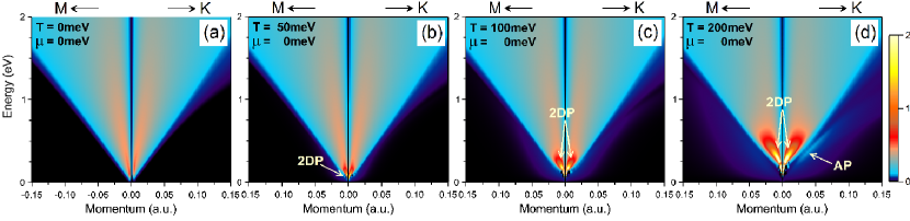
Figure 1: (Color online) Emergence of the 2D plasmon upon increasing the temperature of the electron system in undoped graphene. The excitation spectra, $L({\bf q},\omega)$, in the $\Gamma$M and $\Gamma$K directions evaluated at temperatures of (a) 0, (b) 50, (c) 100, and (d) 200 meV are presented. The borders of a region corresponding to the inter-band e-h pair excitations are maintained almost intact upon variation of $T$, whereas those for the intra-band e-h excitations rapidly expand with $T$ increase. A 2D plasmon (2DP) is observed at all chosen finite temperatures with frequency dispersion $\omega_{2DP}\propto q^{1/2}$ at small $q$’s.

In Fig. 1, we demonstrate how the 2D plasmon emerges in undoped graphene when the temperature of its electron system is increased. Figure 1(a) shows that at $T=0$ the excitation spectrum for low energies is governed by the incoherent e-h pairs involving inter-band transitions between the $\pi$ and $\pi^{\ast}$ energy bands which are the only excitations permitted in this energy interval. However, at finite temperature the 2D plasmon starts to emerge on the low-energy side. Thus, from Fig. 1(b), it is clear that at $T=50$ meV there is a peak in the loss function at energies below approximately 150 meV. The dispersion of this mode presents a clear behavior of a 2D plasmon mode, i.e. its energy goes to zero with the momentum magnitude $q$ reduction as $\propto q^{1/2}$ which is a characteristic of a 2D plasmon. However, there is a substantial difference in comparison with the conventional 2D plasmon case. It consists in that intrinsically the 2D plasmon peak in the finite $T$ case has finite linewidth (e.g. finite lifetime) at any $q$, whereas in the conventional 2D electron gas stprl67 there is an energy threshold below which the 2D plasmon has infinite lifetime (zero linewidth). This difference is explained by the fact that in the finite-$T$ case the restrictions on the phase-space for the e-h pair excitations are relaxed in comparison with the $T=0$ case with the free-carriers stprl67 ; anformp82 . From Fig. 1(b) it is evident that the finite width of the 2D plasmon peak is due to decay into inter-band e-h pairs since its dispersion occurs above the intra-band e-h pair continuum, as it appears in a conventional 2D electron gas at $T=0$. However, even though at finite $T$ there is not a well-defined low-energy border for the inter-band region, it is seen in Fig. 1(b) how the 2D plasmon width is increased as its energy is increased. Finally, at $\omega$ around 150 meV, the decay into the inter-band e-h pairs becomes so efficient that at larger energies this mode ceases to be a well-defined collective excitation.

Upon increasing the temperature, the number of free carriers in the system is also increased. This fact is reflected in the 2D plasmon dispersion relation which is blue shifted as one can see from comparison of the T=50, 100, and 200 meV plots presented in Figs. 1(b), (c), and (d), respectively. Even though the region for the intra-band e-h excitations is expanded when $T$ is increased, the dispersion relation of 2D plasmons occurs over an expanded phase-space as $T$ grows. Therefore, in Figs. 1(c) and (d), one can resolve a well-defined peak corresponding to the 2D plasmon up to energies of $\approx 350$ and $\approx 650$ meV for the T=100 and 200 meV cases, respectively.

From Fig. 1, it is easy to perceive that the shape of the e-h continua for the intra- and inter-band e-h pair excitations are visibly anisotropic in this momentum-energy range. However, the 2D plasmon dispersion relation for the corresponding temperatures is almost isotropic and is in good agreement with results from a simple model employing the DCA daliprb13 . This may be explained by noting that the 2D plasmon dispersion relation for small momenta transfer is determined stprl67 by the total number of free carriers which does not depend on the momentum direction for the Dirac cone at low energies and the role played by other factors such as the inter-band transitions is of less importance.

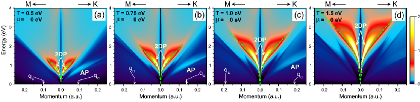
Figure 2: (Color online) Evolution of the 2D plasmon dispersion relation upon increasing the temperature of the electron system in undoped monolayer graphene. The excitation spectra, $L({\bf q},\omega)$, in the $\Gamma$M and $\Gamma$K directions evaluated at $T$ equal to (a) 0.5, (b) 0.75, (c) 1.0, and (d) 1.5 eV. A 2D plasmon (2DP) is observed for all these chosen temperatures with energy dispersion $\omega_{2DP}\propto q^{1/2}$. Green dashed lines demonstrate the 2D plasmon dispersion obtained in the DCA daliprb13 and occurring at $q$’s smaller than a cut-off momentum $q_{c}$.

Upon further $T$ increase, there are significant changes in the excitation spectrum of undoped graphene. These are produced by the strong trigonal warping of the energy bands forming the Dirac cone at energies exceeding $\approx 300$ meV. In Fig. 2, we compare the excitation spectrum calculated at $T=0.5$, 0.75, 1.0, and 1.5 eV. By noting the dissimilarity between Fig. 2(a) with Fig. 1(d), one notices that an increase in $T$ from 200 meV to 500 meV drastically increases the size of the region for the intra-band e-h transitions with a corresponding increase in the number of free carriers in the systems. This results in an increase in the 2D plasmon strength at $T=0.5$ eV accompanied by a notable upward shift in its energy. Despite the increase in the number of e-h excitations in this region, the 2D plasmon peak is well defined over an extended energy range up to $\approx 1.5$ eV. In Fig. 2, we also plot the 2D dispersion evaluated in the framework of a DCA. One can see in Fig. 2(a) that our 2D plasmon dispersion relation almost coincides with the DCA model predictions of Ref. daliprb13 . Moreover, the momentum range where this mode can be a well-defined collective excitation is almost the same in both models. This demonstrates that the DCA is capable of describing the 2D plasmon behaviors even at such elevated temperatures. However, upon further increase of $T$, notable deviations in our calculated 2D plasmon dispersion relations from the simple model predictions become noticeable. Thus, in Fig. 2(b), one can see that our calculated 2D plasmon dispersion relation goes to slightly higher energy in comparison with the DCA model curve represented by green dashed lines. Moreover, at such elevated temperatures, some anisotropy in the 2D plasmon dispersion becomes evident. Upon further temperature increase, these main deviations of our 2D plasmon dispersion relation from the simple model curves increase as evidenced from the loss function for $T=1.0$ and 1.5 eV reported in Figs. 2(c) and 2(d), respectively. Thus, in the $T=1.5$ eV case of Fig. 2(d), our calculated 2D energy dispersion exceeds that obtained in the simple model by about 15 $\%$. We attribute this deviation of our 2D plasmon dispersion to the predictions in Ref. daliprb13 to the presence of other energy bands in the graphene band structure which are thermally populated at such elevated $T$’s. As a result, the number of carriers at finite $T$ is increased additionally due to a partial occupation of the $\sigma$ bands, high density-of-states in the $\pi$ and $\pi^{*}$ bands in the vicinity of the M point, and image states sizhprb09 . Also, the anisotropy of the 2D plasmon dispersion becomes more notable with the temperature increase. This behavior can also be explained by increased deviation of the density of states in graphene pisinjp14 at increasing energy separation from the Dirac point in comparison with that assumed in the DCA.

Close examination of Fig. 1(d) reveals that for momentum transfers in a 0.02-0.07 a.u. range along the $\Gamma$K direction a faint peak referred to as an acoustic plasmon (AP) mode appears at energies below the 2D plasmon. We explain its presence by the fact that at such temperature some amount of slow carriers can be excited in addition to those moving with $v_{F}\approx 0.4$ a.u. as can be seen in Fig. 4(d) of Ref. pisinjp14 . As a result, a two-component electron gas scenario may be realized in graphene at this $T$ even in the case when the chemical potential is pinned at the Dirac point. As demonstrated by the models, the dispersion of the AP mode picjp56 should have an acoustic-like law, i.e., its energy decays as $\sim q$ upon reduction of momentum magnitude $q$. From Fig. 1(d), it is clear that the AP plasmon dispersion relation in graphene deviates significantly from such behavior. Nevertheless, in order to stress its origin we apply the term “acoustic plasmon” to this mode as well. When the temperature is increased, the number of both slow and fast carriers increases as well, making the phenomenon of the AP even more clear as evidenced from the loss spectrum for $T=0.5$ eV of Fig. 2(a), where an AP peak can be discerned along the $\Gamma$K at $q$’s exceeding $\approx 0.03$ a.u.

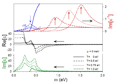
Figure 3: (Color online) The real and imaginary parts of the dielectric function $\epsilon({\bf q},\omega)$ as well as the energy loss function $L({\bf q},\omega)$ for some values of temperature at $\mu=0$. The data are for wave vector directed along the $\Gamma$K directions with $q=0.038$ a.u. In the upper panel at energies below 0.6 eV the blue lines show the loss function multiplied by a factor 10. Blue vertical arrow marks the energy position of the AP mode. Red vertical arrows mark the energy positions of the 2DP.

In order to demonstrate the origin of the AP mode, we present in Fig. 3 the $\omega$-dependence of the real and imaginary parts of the dielectric function as well as the loss function calculated for $\mu=0$ and various temperatures $T$ at $q=0.038$ a.u. along $\Gamma$K. The zeros of Re$[\epsilon]$ correspond to the plasmon excitation frequencies while the Im$[\epsilon]$ gives the Landau damping. As a matter of fact, an undamped plasmon mode occurs at a frequency when “both” the real and imaginary parts of the dielectric function are zero. However at the chosen temperatures the imaginary part of the dielectric function is zero only for $T=0$ at energies below the threshold $\omega_{t}=0.35$ eV for the interband $\pi$-$\pi^{*}$ transitions for this ${\bf q}$. In all other cases, it is finite at the non-zero $\omega$’s. Nevertheless, the energy loss function displays peaks, each arising at a frequency where there is either a 2D plasmon or an AP mode. The height of each peak for the loss function is representative of the intensity of the plasmon excitation mode. We note that the imaginary part of $\epsilon({\bf q},\omega)$ in Fig. 3 becomes larger on the low-energy side as the temperature is increased, which reflects the increasing number of charge carriers. There is a corresponding modification of the real part. A consequence of this behavior is a rapid increase in the energy of the 2D plasmon when the temperature is raised. In the low-energy part of Im$[\epsilon]$ at $T=0.5$ eV of Fig. 3 one can see that instead of a single peak seen at $\omega=0.42$ eV in the $T=0$ case there are two peaks at energies below 1 eV. Their appearance is related, as explained above, to the intra-band transitions involving two kinds of carriers moving with different group velocities in the $\Gamma$K direction pisinjp14 . This makes the real part of $\epsilon$ cross the zero axis additionally twice in this energy interval. Such zero-crossings together with existence of a local minimum in Im$[\epsilon]$ leads to the appearance of a peak in the loss function at $\omega=0.35$ eV that signals the existence of the AP mode at this energy. Upon the increase in temperature, the strength of both peaks in Im$[\epsilon]$ gradually increases due to an increased number of free carriers in the system. This is accompanied by the upward shift of Re$[\epsilon]$ at $\omega$ less than 0.45 eV as seen in the curves corresponding to $T=0.75$ and 1.0 eV. Consequently, the condition for the existence of a well-defined collective AP mode is relaxed. This is confirmed by a gradual reduction of the spectral weight of the AP peak in the loss function at these $T$’s.

Viewing closely the loss spectra in Figs. 1 and 2 reveals that a peak corresponding to the AP mode does not appear along the $\Gamma$M direction. As in the case for extrinsic doping which was considered in Ref. pisinjp14 and in what follows, its absence in this direction is attributed to the presence of only one kind of carriers moving in this direction for the energy interval from -1 eV to +1 eV as seen in Fig. 4(d) of Ref. pisinjp14 . This is confirmed by Fig. 4 where we report the real and imaginary parts of the dielectric function and the loss function calculated for $\mu=0$ and various temperatures $T$ at $q=0.044$ a.u. along $\Gamma$M. Since, in this direction there is only one kind of carriers, the Im$[\epsilon]$ presents only a single intra-band peak at finite $T$’s. Consequently, the real part of $\epsilon$ crosses the zero axis only once at energies around $\omega=0.45$ eV where Im$[\epsilon]$ possesses a peak. As a result, the corresponding mode cannot be realized since it is Landau-damped. This is confirmed by the absence of any peak in the nearby energy region in the loss function. Instead, in it only the peak corresponding to the conventional 2DP mode is observed at higher energies.

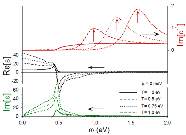
Figure 4: (Color online) The real and imaginary parts of the dielectric function $\epsilon({\bf q},\omega)$ as well as the energy loss function $L({\bf q},\omega)$ for some values of temperature at $\mu=0$. The data are for wave vector directed along the $\Gamma$M directions with $q=0.044$ a.u. The red vertical arrows mark the energy positions of the 2DP.

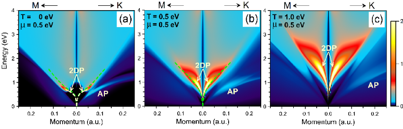
Figure 5: (Color online) Excitation spectra, $L({\bf q},\omega)$, in the $\Gamma$M and $\Gamma$K directions evaluated at $\mu=0.5$ eV and $T$ of (a) 0, (b) 0.5 and (c) 1.0 eV. The 2D plasmon (2DP) and acoustic plasmon (AP) dispersions are denoted by corresponding labels. Yellow dashed lines show the undamped 2DP dispersion. Green dashed lines demonstrate the 2D plasmon dispersion obtained in the DCA model daliprb13 .

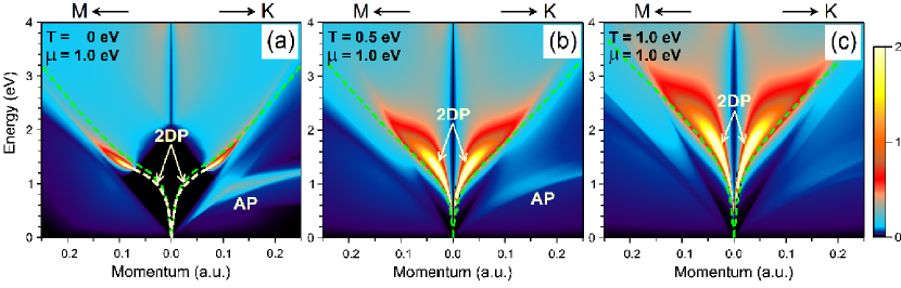
Figure 6: (Color online) Excitation spectra, $L({\bf q},\omega)$, in the $\Gamma$M and $\Gamma$K directions evaluated at $\mu=1.0$ eV and $T$ of (a) 0, (b) 0.5 and (c) 1.0 eV. The 2D plasmon (2DP) and acoustic plasmon (AP) dispersions are denoted by corresponding labels. Yellow dashed lines show the undamped 2DP dispersion. Green dashed lines demonstrate the 2D plasmon dispersion obtained in the DCA model daliprb13 .

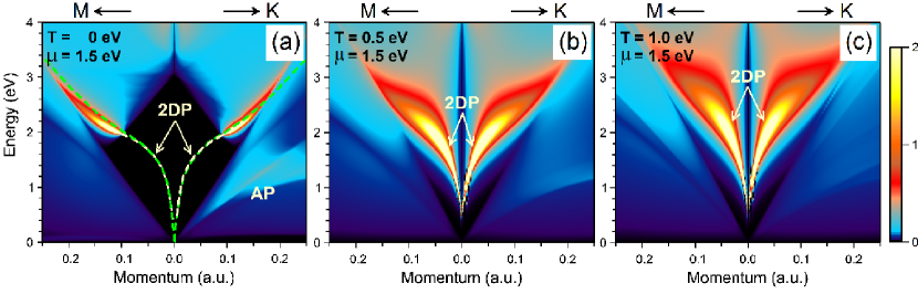
Figure 7: (Color online) Excitation spectra, $L({\bf q},\omega)$, in the $\Gamma$M and $\Gamma$K directions evaluated at $\mu=1.5$ eV and $T$ of (a) 0, (b) 0.5 and (c) 1.0 eV. The 2D plasmon (2DP) and acoustic plasmon (AP) dispersions are denoted by corresponding labels. Yellow dashed lines show the undamped 2DP dispersion. Green dashed lines demonstrate the 2D plasmon dispersion obtained in the DCA model daliprb13 .

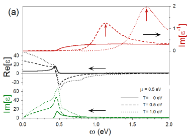
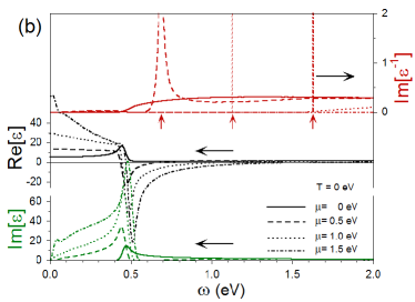
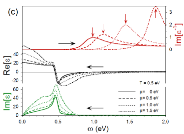
Figure 8: (Color online) The real and imaginary parts of the dielectric function $\epsilon({\bf q},\omega)$ as well as the energy loss function, $L({\bf q},\omega)$, for some values of doping and temperature. The data are for wave vector directed along the $\Gamma$M direction with $q=0.044$. The chemical potential level $\mu$ and temperature $T$ are as follows: (a) $\mu=0.5$ eV and various $T$, (b) $T=0$ and various $\mu$, (c) $T=0.5$ eV and various $\mu$. Red vertical arrows mark the energy positions of the 2DP.

It is interesting to compare the spectra reported in Fig. 2 with those corresponding to the cases with non-zero doping $\mu$ upon the temperature change. These data for $\mu=0.5$, 1.0, and 1.5 eV are reported in Figs. 5, 6 and 7, respectively. Figures 5(a), 6(a), and 7(a) demonstrate the behavior of the energy-loss spectra at zero temperature as the doping level is increased from $0.5$ to $1.5$ eV, i.e., expanding the $0-1.0$ eV energy range explored at zero temperature in previous publication pisinjp14 . From the $1.5$ eV panel in Fig. 7(a), it is clear that the 2D plasmon also exists even at such a high doping level. At small momenta, the 2D plasmon dispersion frequency is enhanced due to an increased carriers number at the corresponding Fermi level. In contrast to the loss spectra for $\mu=0$ and $T\neq 0$ of Fig. 2 the 2D plasmon peak in Figs. 5(a), 6(a), and 7(a) has zero width over the extended phase space momentum-energy region, as highlighted by yellow dashed line. One can observe how this region where the 2D mode is undamped is gradually increased upon shifting the position of $\mu$ at energy as high as 1.5 eV. At such doping level the 2D plasmon does not decay into e-h pairs up to energy of $\approx 2$ eV. In Figs. 5(a), 6(a) and 7(a) with green dashed lines, we show the 2DP dispersion predicted by the DCA model daliprb13 which clearly does not depend on the momentum direction. From comparison of the 2DP dispersion calculated here with these curves one can observe its notable asymmetry. Moreover, apparently the momentum (and energy) range where this mode is a well defined collective excitation is significantly smaller than that predicted employing the DCA. It may signal that this model underestimates the decay rate of the 2DP into e-h pairs.

Additionally, from the excitation spectrum reported in Fig. 7(a), one can deduce that the AP mode also exists at $\mu=1.5$ eV along the $\Gamma$K direction, even though the width of the corresponding peak in the loss function is notably increased in comparison to the $\mu=0.5$ and 1.0 eV cases indicating that with the doping level greater than $1.0$ eV, this mode more efficiently decays into incoherent e-h pairs. Its dispersion is linear at values of $q$ reaching $0.25$ a.u. which is in contrast to the $\mu=0.5$ and 1.0 eV cases, where it starts to deviate from the linear dispersion at significantly lower $q$’s.

Figures 5, 6, and 7 explore the “combined” effect of temperature and doping on the Coulomb excitations in monolayer graphene. These results clearly demonstrate the novelty and importance of our studies through our modeling and extensive numerical calculations. Our comprehensive studies predict an unusual and diverse behavior of the many-body properties for doped and undoped graphene at finite temperature. There is a 2DP mode in all panels for both $\Gamma$M and $\Gamma$K directions for all values of doping and temperature studied here. For some finite values of $T$ our calculated 2DP dispersion can be compared with the one predicted by the DCA approximation of daliprb13 . In general, the agreement between two models is rather good, although a prominent anisotropy in the 2DP dispersion obtained in the full calculations is evident. Another observation in Figs. 5, 6 and 7 consists in that at finite $T$’s the 2DP dispersion obtained here is always blue shifted in comparison that predicted by the DCA. We explain such behavior by the deviation of graphene band structure from the DCA upon energy separation from the Dirac point. Interestingly, in the $T=0$ case of Figs. 5, 6, and 7, our 2DP dispersion over extended momentum range goes at slightly lower energies in comparison with that generated by the DCA model.

In Fig. 8(a), we present some detailed results for the real and imaginary parts of the dielectric function along with the energy loss function for doping $\mu=0.5$ eV and various temperatures. Again, the location of the peak in the loss function for the 2D plasmon excitation energy gets shifted upward rapidly as the temperature is increased due to a substantial increase in the Drude peak of Im$[\epsilon]$, which is indicative of a swift increase in the number of carriers that are thermally excited. This may be accounted for by the corresponding shift in the density-of-states away from the Dirac point. The dependence of the dielectric properties of graphene upon doping at $T=0$ K is also worth investigating. Figure 8(b) (again, data for $q=0.044$ a.u. along $\Gamma$M) shows this for undoped graphene along with four chosen doping values. Regarding the combined effect arising from temperature and doping on the 2D plasmon excitation spectrum, we present Fig. 8(c). In general, when $T$ and $\mu$ are increased, the 2D plasmon frequency is increased.

In Figs. 5, 6, and 7 one can observe how the AP peak in the loss function corresponding to the acoustic plasmon mode gradually washed out from the calculated loss spectra upon the $T$ increase. In Figs. 5, 6, and 7, the AP branch is suppressed when the values for the doping and temperature are simultaneously large. Additionally, one can see that the intensity of the AP branch is decreased as the doping level exceeds 1.0 eV. A general tendency is that this mode ceases to exist at a lower $T$ value as the doping level is increased. Thus, in Fig. 5 at $\mu=0.5$ eV the AP peak can be detected at all the temperature reaching 1.0 eV. In Fig. 6 one can see that at $\mu=1.0$ eV the AP peak is well defined at $T=0$, being strongly damped at $T=0.5$ eV. Its presence in the $T=1.0$ eV spectrum is barely visible, demonstrating that can not exist at such combination of $\mu$ and $T$. From Fig. 7 corresponding to case of the 1.5 eV doping, the AP peak is completely removed from the $T=1.0$ eV loss spectrum of Fig. 7(c). At such elevated doping level the peak originally corresponding to the AP mode is so broad at $T=0.5$ eV of Fig. 7(b) that it can not be considered as a well-defined collective excitation. Disappearance of the AP mode in graphene at significantly lower temperature upon increase of the doping level (accompanied by the strong increase of number of carriers at the Fermi level) correlates with effective destruction of the AP mode in bulk Pd at significantly lower temperatures as was reported recently sinaprb16 .

IV Concluding Remarks

In summary, we have employed the density functional method to calculate the electronic energy bands for graphene in the absence of an external magnetic field. Using these results, we calculated the longitudinal wave vector and frequency-dependent dielectric function at arbitrary temperature. In our calculations, the entire energy band spectrum was included. This ensures the correctness of the dielectric function in the RPA and consequently the plasmon intensity and its frequency. We presented the plasmon excitation spectra at various temperatures and doping concentrations which may be achieved experimentally. Our method may also be applicable to other rare 2D materials with Dirac cones such as silicene, germanene and graphyne over a wide range of temperature and doping. Our numerical results may be validated by inelastic light-scattering or high-resolution electron-energy loss spectroscopy which has been successfully applied to the two-dimensional electron gas system.

V Acknowledgments

V.M.S acknowledges the partial support from the University of the Basque Country UPV/EHU, Grant No. IT-756-13 and the Spanish Ministry of Economy and Competitiveness MINECO, Grant No. FIS2016-76617-P.

References

- (1) G. Dresselhaus, Phys. Rev. B 10, 3602 (1974).
- (2) K. Nakao, J. Phys. Soc. Jpn 40, 761 (1976).
- (3) J. C. Charlier, J. P. Michenaud, X. Gonze, and J. P. Vigneron, Phys. Rev. B 44, 13237 (1991).
- (4) J. C. Charlier, X. Gonze, and J. P. Michenaud, Phys. Rev. B 43, 4579 (1991).
- (5) J. C. Charlier, J. P. Michenaud, and X. Gonze, Phys. Rev. B 46, 4531 (1992).
- (6) U. Büchner, Phys. Status Solidi (b) 81, 227 (1977).
- (7) C. Kramberger, R. Hambach, C. Giorgetti, M. H. Rummeli, M. Knupfer, J. Fink, B. Büchner, Lucia Reining, E. Einarsson, S. Maruyama, F. Sottile, K. Hannewald, V. Olevano, A. G. Marinopoulos, and T. Pichler, Phys. Rev. Lett. 100, 196803 (2008).
- (8) J. Lu, K. P. Loh, H. Huang, W. Chen, and A. T. S. Wee, Phys. Rev. B 80, 113410 (2009).
- (9) C. Kramberger, E. Einarsson, S. Huotari, T. Thurakitseree, S. Maruyama, M. Knupfer, and T. Pichler, Phys. Rev. B 81, 205410 (2010).
- (10) S. Z. Butler at al., ACS Nano 7, 2898 (2013).
- (11) M. Xu, T. Liang, M. Shi, and H. Chen, Chem. Rev. 113, 3766 (2013).
- (12) P. R. Wallace, Phys. Rev. 71, 622 (1947).
- (13) B. Wunsch, T. Stauber, F. Sols, and F. Guinea, New J. Phys. 8, 318 (2006).
- (14) E. H. Hwang and S. Das Sarma, Phys. Rev. B 75, 205418 (2007).
- (15) F. H. Koppens, D. E. Chang, and F. J. Garcia de Abajo, Nano Lett. 11, 3370 (2011).
- (16) J. Chen el al., Nature 487, 77 (2012).
- (17) Z. Fei el al., Nature 487, 82 (2012).
- (18) A. N. Grigorenko, M. Polini, and K. S. Novoselov, Nature Phot. 6, 749 (2012).
- (19) M. Freitag, T. Low, W. J. Zhu, H. G. Yan, F. N. Xia, and P. Avouris, Nature Commun. 4, 1951 (2013).
- (20) F. J. Garcia de Abajo, ACS Phot. 1, 135 (2014).
- (21) D. Rodrigo, O. Limaj, D. Janner, D. Etezadi, F. J. Garcia de Abajo, V. Pruneri, and H. Altug, Science 349, 165 (2015).
- (22) T. Stauber, J. Schliemann, and N. M. R. Peres, Phys. Rev. B 81, 085409 (2010).
- (23) Y. Gao and Z. Yuan, Solid State Commun. 151, 1009 (2011).
- (24) V. Despoja, D. Novko, K. Dekanić, M. Šunjić, and L. Marušić, Phys. Rev. B 87, 075447 (2013).
- (25) M. Pisarra, A. Sindona, P. Riccardi, V. M. Silkin, and J. M. Pitarke, New J. Phys. 16, 083003 (2014).
- (26) A. Politano and G. Chiarello, Carbon 71, 176 (2014).
- (27) J. C. Slonczewski and P. R. Weiss, Phys. Rev. 109, 272 (1958).
- (28) J. W. McClure, Carbon 7, 425 (1969).
- (29) D. Pines, Can. J. Phys. 34, 1379 (1956).
- (30) V. M. Silkin, A. Garcia-Lekue, J. M. Pitarke, E. V. Chulkov, E. Zaremba, and P. M. Echenique, Europhys. Lett. 66, 260 (2004).
- (31) Y. Liu, R. F. Willis, K. V. Emtsev, and T. Seyller, Phys. Rev. B 78, 201403 (2008).
- (32) H. Pfn’́ur, T. Langer, J. Baringhaus, and C. Tegenkamp, J. Phys.: Condens. Matter 23, 112204 (2011).
- (33) S. Y. Shin, C. G. Hwang, S. J. Sung, N. D. Kim, H. S. Kim, and J. W. Chung, Phys. Rev. B 83, 161403(R) (2011).
- (34) S. Y. Shin, N. D. Kim, H. S. Kim, K. S. Kim, D. Y. Noh, K. S. Kim, and J. W. Chung, Appl. Phys. Lett. B 99, 082110 (2011).
- (35) T. Langer, H. Pfnür, C. Tegenkamp, S. Forti, K. Emtsov, and U. Starke, New J. Phys. 14, 103045 (2012).
- (36) A. Politano, A. R. Marino, V. Formoso, D. Fariás, R. Miranda, and G. Chiarello, Phys. Rev. B 84, 033401 (2011).
- (37) A. Politano, A. R. Marino, and G. Chiarello, Phys. Rev. B 86, 085420 (2012).
- (38) A. Politano, V. Formoso, and G. Chiarello, J. Phys.: Condens. Mat. 25, 345303 (2013).
- (39) A. Politano and G. Chiarello, Nanoscale 6, 10927 (2014).
- (40) T. Langer, D. F. Forster, C. Busse, T. Michely, and H. Pfnür, New J. Phys. 13, 053006 (2011).
- (41) N. J. M. Horin, A. Iurov, G. Gumbs, A. Politano, and G. Chiarello, Recent Progress in Nonlocal Graphene Plasmons in Low-Dimensional and Nanostructured Materials and Devices (Springer, 2015) pages 205-237.
- (42) V. Borka Jovanović, I. Radović, D. Borka, and Z. L. Mišković, Phys. Rev. B 84, 155416 (2011).
- (43) C. Gong, S. McDonnell, X. Qin, A. Azcatl, H. Dong, Y. J. Chabal, K. Chao, and R. M. Wallace, ACS Nano 8, 642649 (2013).
- (44) S. Das Sarma and Q. Li, Phys. Rev. B 87, 235418 (2013).
- (45) F. Stern, Phys. Rev. Lett. 18, 546 (1967).
- (46) D. Pines and P. Nozières, The Theory of Quantum Liquids: Normal Fermi Liquids (W. A. Benjamin, New York, 1966), Vol. 1.
- (47) D. M. Ceperley and B. J. Alder, Phys. Rev. Lett. 45, 566 (1980), as parametrized by J. P. Perdew and A. Zunger, Phys. Rev. B 23, 5048 (1981).
- (48) N. Troullier and J. L. Martins, Phys. Rev. B 43, 1993 (1991).
- (49) V. M. Silkin, E. V. Chulkov, and P. M. Echenique, Phys. Rev. B 68, 205106 (2003).
- (50) E. Runge and E. K. U. Gross, Phys. Rev. Lett. 52, 997 (1984).
- (51) M. Petersilka, U. J. Gossmann, and E. K. U. Gross, Phys. Rev. Lett. 76, 1212 (1996).
- (52) H. Ehrenreich and M. H. Cohen, Phys. Rev. 115, 786 (1959).
- (53) V. M. Silkin, E. V. Chulkov, and P. M. Echenique, Phys. Rev. Lett. 93, 176801 (2004).
- (54) B. Diaconescu, K. Pohl, L. Vattuone, L. Savio, P. Hofmann, V. M. Silkin, J. M. Pitarke, E. V. Chulkov, P. M. Echenique, and M. Rocca, Nature 448, 57 (2007).
- (55) J. Yan, K. W. Jacobsen, and K. S. Thygesen, Phys. Rev. B 86, 241404(R) (2012).
- (56) A. Bergara, V. M. Silkin, E. V. Chulkov, and P. M. Echenique, Phys. Rev. B 67, 245402 (2003).
- (57) V. U. Nazarov, New J. Phys. 17, 073018 (2015).
- (58) P. F. Maldague, Surf. Sci. 73, 296 (1978).
- (59) T. Ando, A. B. Fowler, and F. Stern, Rev. Mod. Phys. 54, 437 (1982).
- (60) V. M. Silkin, J. Zhao, F. Guinea, E. V. Chulkov, P. M. Echenique, and H. Petek, Phys. Rev. B 80, 121408 (2009).
- (61) V. M. Silkin, V. U. Nazarov, A. Balassis, I. P. Chernov, and E. V. Chulkov, Phys. Rev. B 94, 165122 (2016).