Wind-accelerated orbital evolution in binary systems with giant stars

Abstract

Using 3D radiation-hydrodynamic simulations and analytic theory, we study the orbital evolution of asymptotic-giant-branch (AGB) binary systems for various initial orbital separations and mass ratios, and thus different initial accretion modes. The time evolution of binary separations and orbital periods are calculated directly from the averaged mass loss rate, accretion rate and angular momentum loss rate. We separately consider spin-orbit synchronized and zero spin AGB cases. We find that the the angular momentum carried away by the mass loss together with the mass transfer can effectively shrink the orbit when accretion occurs via wind-Roche-lobe overflow. In contrast, the larger fraction of mass lost in Bondi-Hoyle-Lyttleton accreting systems acts to enlarge the orbit. Synchronized binaries tend to experience stronger orbital period decay in close binaries. We also find that orbital period decay is faster when we account for the nonlinear evolution of the accretion mode as the binary starts to tighten. This can increase the fraction of binaries that result in common envelope, luminous red novae, Type Ia supernovae and planetary nebulae with tight central binaries. The results also imply that planets in the the habitable zone around white dwarfs are unlikely to be found.

1 Introduction

Binary systems are progenitors for a wide range of astrophysical systems given the multiplicity of evolutionary outcomes. For much of a binary’s lifetime, the component stars may be non-interacting. However when one of the star evolves to the red giant branch (RGB) or asymptotic giant branch (AGB), the stars may interact via wind-mass transfer and/or tidal friction (Zahn, 1977); their subsequent mutual evolution is strongly coupled (Paczyński, 1971).

The mass transfer interaction can be classified into four types in increasing order of interaction. These are: Bondi-Hoyle-Lyttleton (BHL) accretion (Hoyle & Lyttleton, 1939; Bondi & Hoyle, 1944; Edgar, 2004); wind-Roche-lobe overflow (WRLOF) (Podsiadlowski & Mohamed, 2007); Roche-lobe overflow (RLOF) (Paczyński, 1971); and common envelope (CE) (Ivanova et al., 2013). Secular and dynamical instabilities can develop before the Roche limit contact is reached, which may in turn propel the system into the RLOF regime (Lai et al., 1994).

The aforementioned mass transfer modes are commonly studied separately, but they are often successive stages of time-evolving systems. For example, RLOF and tidal friction (TF) can shrink the orbit (Tout & Hall, 1991; Lai et al., 1994) and may lead to CE when both stars’ Roche lobes are filled. As we will see, at even larger initial separations, WRLOF can effectively transfer mass between binary stars while depositing angular momentum into a circumbinary disc. The system can then evolve to RLOF as the binary orbit shrinks. This exemplifies how these three modes of mass transfer can be connected by orbital period decay (OPD). As we suggest herein, a sufficiently rapid evolution to the CE stage, even from widely separated binaries, implies that there may be many more binary systems that can ultimately arrive at CE than would be estimated using only their initial separation.

Example systems which result from binary interactions for which our study is germane include, luminous red novae (LRNe), type Ia supernovae (SNe), and planetary nebulae (PNe). LRNe have luminosities lower than typical supernovae that occur on white dwarfs (WD) but higher than novae. LRN light curves peak in the optical before the infrared. Since 1989 (Rich et al., 1989), many new LRNe have been observed: M31RV (Rich et al., 1989), V4332 Sgr (Martini et al., 1999), V838 Mon (Brown et al., 2002; Bond et al., 2003; Munari et al., 2005; Tylenda, 2005), M85 OT2006-1 (Kulkarni et al., 2007; Rau et al., 2007), V1309 Scorpii (Tylenda et al., 2011) and the recent M31LRN 2015 (MacLeod et al., 2017). Their origin is not fully understood; some may be caused by a helium flash while others may result from merging binary systems (Pejcha et al., 2016; Staff et al., 2016; Metzger & Pejcha, 2017). For the latter ’mergeburst’ scenario, it is believed that the binary system will incur a CE (Nordhaus & Blackman, 2006; Ivanova et al., 2013). During this phase, a considerable fraction of the envelope may be ejected or pushed to larger orbits. When the central binary sufficiently tightens or merges, kinetic energy will be released and the ejected envelope will be heated. Prior to the CE phase, there would also be a phase of RLOF. RLOF and CE phases also likely precede Type Ia SNe (Iben & Tutukov, 1984; Kenyon et al., 1993; Ivanova et al., 2013; Santander-García et al., 2015).

PNe are the nebular end states of low-mass stars (Han et al., 1995). PNe have been observed to have a range of shapes, mostly aspherical, and often bipolar and asymmetric (Balick & Frank, 2002). Many PNe might be explained by binary models (Soker & Livio, 1994; Mastrodemos & Morris, 1998; Nordhaus & Blackman, 2006; Hillwig et al., 2016; Chen et al., 2017; Kim et al., 2017) but some might require triples (Bear & Soker, 2017).Some PNe have WD-WD binaries in the central region Santander-García et al. (2015); Miszalski et al. (2017). In rapidly evolving binary system, magnetic fields can be an intermediary in the conversion of rotational energy into jets and asymmetric outflows (Nordhaus et al., 2007; Nordhaus et al., 2011). All of this highlights the importance of assessing how binary systems evolve as a function of initial conditions.

Another interesting context for our study is the effort to determine what kind of binary systems with planets or secondaries survive around WD. Villaver & Livio (2009) and (Nordhaus et al., 2010) investigated the orbital change in low-mass binary systems and found that tidal friction, gravitational drag and mass loss from the primary are responsible for orbital change. Given the engulfment of low-mass companions during the giant phase of the primary, Nordhaus & Spiegel (2013) found that planetary companions will be tidally disrupted during the CE phase and thus not remain intact in close orbits around WDs. For these systems, engulfment by CE is likely in the final stages of OPD, but may have been preceded by RLOF and WRLOF. RLOF and WRLOF are fundamentally different from BHL, the latter being the mass transfer mode assumed by Villaver & Livio (2009).

With CE being such a key final stage determining the phenomenology of many stellar and planetary systems, a basic question is to understand how wide initial binary systems can be and still arrive at CE. In particular what binary systems incur WRLOF and RLOF on the path to CE? If the evolution through these stages is rapid enough (for example, shorter than an AGB stellar lifetime), then even systems with initial separations outside of a CE, might evolve to CE. We explore this in the present paper. The results are important for improving the statistics of binary evolution.

Our study combines our previous 3D radiation hydrodynamic simulations of WRLOF and BHL accretion in AGB binary systems, with analytic theory. In Section 2, we briefly describe the numerical model of our simulations. In Section 3, we present the analytic model of synchronized and non-synchronized binaries. In Section 4, we apply the numerical results from simulations to the analytic model to characterize the orbital period change rate in realistic AGB binary systems. We then compare the results with both conservative mass transfer systems and ideal BHL mass transfer systems. In Section 5, we discuss the phenomenological implications. We conclude in Section 6.

2 Numerical Model

A detailed description of the numerical model can be found in Chen et al. (2017). Here we outline the salient features for the present simulations.

The 3D radiation hydrodynamic simulations, performed with ASTROBEAR (Cunningham et al., 2009; Carroll-Nellenback et al., 2013), are carried out in the co-rotating frame of the binary systems (table 6). When the boundary of the giant star is stationary in the co-rotating frame, the giant star is in spin-orbit synchronized rotation in the lab frame (Appendix A). In addition, a 2D ray tracing algorithm, cooling and dynamic dust formation are considered in these simulations. The wind from the giant star is driven by a piston model at the inner boundary of the giant star and the radiation pressure where dust present. The secondary is accreting the gas (Krumholz et al., 2004).

The numerical models replicate the BHL mode of mass transfer in binaries with large separation and WRLOF mode of mass transfer in close binary systems. The morphology of outflow is similar to some well known objects such as L2 Puppis (Kervella et al., 2016), CIT 6 (Kim et al., 2017) and R Sculptoris (Maercker et al., 2012).

Since the simulations are carried out in Cartesian coordinate with Eulerian code, an important concern is how well angular momentum is conserved. We find that angluar momentum in the wind to be conserved within $4\%$, up to 1.4 times the orbital separation, which is good enough not to affect our conclusions. Detailed analysis can be found in Appendix B.

Although the numerical simulations are carried out in the co-rotating frame as mentioned above, all of our analytic calculations are carried out for the lab frame. We designate subscript ’1’ to the giant star and subscript ’2’ to the secondary.

3 Analytic Model

Boyarchuk et al. (2002) and lecture notes by Pols provide general equations for calculating the evolution of binary separation. Tout & Hall (1991) and Pribulla (1998) also developed analytic models of orbital evolution of binary stars, considering mass transfer, mass loss and angular momentum loss. Here we follow a similar method to derive the orbital period change rate for both synchronized and non-spinning binaries. For present purposes "synchronized" refers to the spin-orbit synchronization of our primary AGB stellar rotation period with the orbital spin, as measured in the lab frame. We do not consider the spin of the secondary.

We assume a binary with primary mass $m_{1}$, secondary mass $m_{2}$, and orbital separation $a$. The z-component of angular momentum of in the lab frame for a fully synchronized state can be expressed by:

$$J=\frac{m_{1}m_{2}(Ga)^{1/2}}{(m_{1}+m_{2})^{1/2}}+\frac{I_{1}(Gm_{1}+Gm_{2})^{1/2}}{a^{3/2}}+\frac{I_{2}(Gm_{1}+Gm_{2})^{1/2}}{a^{3/2}}$$ (1)

where $I_{1}$ and $I_{2}$ are the moment of inertia of each star. $G$ is the gravitational constant.

For binary systems that consist of a giant star and a main sequence star or WD, the giant will contribute most of the moment of inertia. The gas accreted onto the secondary could spin it up and a rapidly spinning secondary could feed back on the accretion. Such feed back warrants a detailed theoretical/numerical model that includes magnetic field and radiation (Springel et al., 2005). Although recognizing that this is important for further work, here we ignore the spin and moment of inertia of the secondary. Equation 1 then becomes

$$J=\frac{m_{1}m_{2}(Ga)^{1/2}}{(m_{1}+m_{2})^{1/2}}+\frac{\alpha_{1}m_{1}R_{1}^{2}(Gm_{1}+Gm_{2})^{1/2}}{a^{3/2}}$$ (2)

Where $\alpha_{1}$ and $R_{1}$ are the moment of inertia factor and radius of the AGB star, respectively. The orbital period of the binary system can be expressed as

$$P=2\pi a^{3/2}(Gm_{1}+Gm_{2})^{-1/2}.$$ (3)

Squaring Eqns. (2) and (3) and taking the time derivative gives

$$2J\dot{J}=A\dot{a}+B,$$ (4)

and

$$2P\dot{P}=\frac{12(a\pi)^{2}\dot{a}}{G(m_{1}+m_{2})}-\frac{4\pi^{2}a^{3}(\dot{m}_{1}+\dot{m}_{2})}{G(m_{1}+m_{2})^{2}},$$ (5)

where

$$\begin{split}A=&\left(\frac{Gm_{1}m_{2}}{\sqrt{Ga(m_{1}+m_{2})}}-\frac{3\alpha_{1}R^{2}m_{1}\sqrt{G(m_{1}+m_{2})}}{a^{5/2}}\right)\\ &\times\left(\frac{\sqrt{Ga}m_{1}m_{2}}{\sqrt{m_{1}+m_{2}}}+\frac{\alpha_{1}R^{2}m_{1}\sqrt{G(m_{1}+m_{2})}}{a^{3/2}}\right)\end{split}$$ (6)

and

$$\begin{split}B=&2\times\left(\frac{\sqrt{Ga}m_{1}m_{2}}{\sqrt{m_{1}+m_{2}}}+\frac{\alpha_{1}R^{2}m_{1}\sqrt{G(m_{1}+m_{2})}}{a^{3/2}}\right)\\ &\times\Bigg{(}\frac{\sqrt{Ga}m_{2}\dot{m}_{1}}{\sqrt{m_{1}+m_{2}}}+\frac{\alpha_{1}R^{2}\dot{m}_{1}\sqrt{G(m_{1}+m_{2})}}{a^{3/2}}+\frac{\sqrt{Ga}m_{1}\dot{m}_{2}}{\sqrt{m_{1}+m_{2}}}\\ &-\frac{\sqrt{Ga}m_{1}m_{2}(\dot{m}_{1}+\dot{m}_{2})}{2\left(m_{1}+m_{2}\right)^{3/2}}+\frac{\alpha_{1}R^{2}G(\dot{m}_{1}+\dot{m}_{2})}{2a^{3/2}\sqrt{G(m_{1}+m_{2})}}\Bigg{)}\end{split}$$ (7)

Given $\alpha_{1},R_{1},\dot{J},\dot{m}_{1}$ and $\dot{m}_{2}$, $\dot{a}$ can be calculated with Eqn. (4) and $\dot{P}$ can be calculated by feeding $\dot{a}$ into Eqn. (5). If the primary has zero spin, taking $\alpha_{1}=0$ gives the appropriate result.

4 Results Using Simulations to Fix Model Parameters

4.1 Extracting Parameters from Simulations

To measuring $\dot{m}_{2}$, we simply keep track of the mass of the secondary in our simulations. For $\dot{m}_{1}$, we need to measure the mass loss from the binary system. We do so by summing up the flux through a spherical sampling shell centered at the center of mass of the binary. The sampling shell is chosen large enough to contain both stars. The mass flux through the sampling shell is not sensitive to the size of the shell since ASTROBEAR uses a conservative scheme to conserve mass strictly. Therefore any convenient radius that is large enough will do Chen et al. (2017).

Choosing a sampling shell to calculate $\dot{J}$ is more subtle. Lin (1977) found that the specific angular momentum of escaping parcels about the binary center of mass will continue to increase when moving outward in the orbital plane. The parcel approaches its final specific angular momentum after it reaches $3$ times the binary separation $a$. MacFadyen & Milosavljević (2008) found a similar result. Therefore, spherical sampling shells with radii $r_{\text{shell}}\leq 3a$ that contain both of the stars may in general give different $\dot{J}$..

Another concern is identifying from whence the escaping mass originates. Usually, mass loss from the L2 and L3 Lagrangian point is thought to be escaping mass. But the Roche potential is not accurate for a very luminous binary system Chen et al. (2017). The L2 or L3 point may move inward or disappear when the luminosity increases. In our 3D simulation, the AGB star is pulsating periodically and the corresponding L2 point is oscillating. Thus there is no easy way to pinpoint specific radii which distinguish escaping mass and non-escaping mass, so the best that one can do is make it as large as possible.

Our use of AMR poses a competing constraint that limits how large we can choose the $\dot{J}$ sampling radius. On one hand, AMR allows us to put more computational resources in the central region of the binary system where the mass transfer warrants extra resolution. On the other hand, we must use a coarse grid at large radii, increasing the error there, especially where inertial forces dominate at large radii. To minimize the angular momentum conservation error (Appendix B), we use spherical sampling shells with $1.3$ times of binary separation, centered at the center of mass of the binary. Such sampling shells contain both L2 and L3 points predicted by standard theory in all of our binary models. Given that escaping gas will continue to gain angular momentum as it moves out, this gives a lower bound on $\dot{J}$.

The mass flux through the sampling shell is given by

$$\dot{m}_{\text{esc}}(t)=\oint\limits_{S(1.3a)}\rho\mathbf{v}\cdot\text{d}\mathbf{S},$$ (8)

where $S$ is the surface of the sampling shell with $r_{\text{shell}}=1.3a$, $\rho$ and $\mathbf{v}$ are the local fluid density and velocity, respectively. and $\dot{m}_{1}(t)=-\dot{m}_{\text{esc}}(t)-\dot{m}_{2}(t)$ by mass conservation.

The total angular momentum flux is

$$\oint\limits_{S(1.3a)}(\rho\mathbf{r}\times\mathbf{v})\cdot\mathbf{\hat{z}}\mathbf{v}\cdot\text{d}\mathbf{S}=-\dot{J}(t),$$ (9)

where $\mathbf{\hat{z}}$ is the unit vector in $z$ direction. This $\dot{J}$ for the gas includes both the spin angular momentum that came from the AGB star and the angular momentum gain interaction with the secondary. For one our cases in Section 4.4, we wil deduct the spin angular momentum from $\dot{J}$. We introduce a dimensionless number

$$\gamma(t)=\frac{\dot{J}(t)}{j_{0}\dot{m}_{\text{esc}}(t)},$$ (10)

where $j_{0}=m_{1}m_{2}(Ga)^{1/2}(m_{1}+m_{2})^{-3/2}$ is the specific orbital angular momentum of the binary and $\gamma$ measures how efficient the escaping gas is in removing angular momentum.

Since $\dot{m}_{1},\dot{m}_{2},\dot{J}$ and $\gamma$ (see Appendix C) are time dependent, we average them as follows before using $\dot{m}_{1}$ and $\dot{J}$ in Eqn. (4):

$$\dot{m}_{1}=\int_{t_{i}}^{t_{f}}\dot{m}_{1}(t)\text{d}t,$$ (11)

$$\dot{m}_{2}=\int_{t_{i}}^{t_{f}}\dot{m}_{2}(t)\text{d}t,$$ (12)

$$\dot{J}=\int_{t_{i}}^{t_{f}}\dot{J}(t)\text{d}t,$$ (13)

and

$$\gamma=\frac{\int_{t_{i}}^{t_{f}}\dot{J}(t)\text{d}t}{j_{0}\int_{t_{i}}^{t_{f}}\dot{m}_{\text{esc}}(t)\text{d}t}=\frac{\dot{J}}{j_{0}(\dot{m}_{1}+\dot{m}_{2})},$$ (14)

where $t_{i}$ and $t_{f}$ are the initial and final sampling time, respectively. In practice, we choose $t_{i}$ when the simulation becomes stable and $t_{f}-t_{i}>9$yr. It turns out that $\gamma$ is a more intuitive number than $\dot{J}$ for comparing the angular momentum loss efficiency between different models. Recovering $\dot{J}$ with Equation (14) is straightforward. Table 1 lists $\dot{m}_{1},\dot{m}_{2}$ and $\gamma$.

model	$\dot{m}_{1}$	$\dot{m}_{2}$	$\gamma$	$r_{\text{shell}}$
	M⊙ yr-1	M⊙ yr-1		au
1	$-2.96\times 10^{-7}$	$1.16\times 10^{-7}$	$7.77\times 10^{0}$	3.9
2	$-3.28\times 10^{-7}$	$1.20\times 10^{-7}$	$2.74\times 10^{0}$	5.2
3	$-2.21\times 10^{-7}$	$4.51\times 10^{-8}$	$1.01\times 10^{0}$	7.8
4	$-2.66\times 10^{-7}$	$8.28\times 10^{-9}$	$9.13\times 10^{-1}$	10.4
5	$-2.61\times 10^{-7}$	$5.85\times 10^{-9}$	$8.03\times 10^{-1}$	13

Table 1: Measured parameters from 3D simulations. The first column lists the binary model number (Table 6). $\dot{m}_{1}$ and $\dot{m}_{2}$ are the mass change rate of the primary and the secondary, respectively. $\gamma$ is the average number calculated by Equation (14). $r_{\text{shell}}$ is the radius of the sampling shell (centered at the center of mass of the two stars) through which the escaping flux is measured.

4.2 Conservative versus BHL mass transfer models

Conservative mass transfer is likely for very close binaries incurring RLOF, while BHL mass transfer is more likely for wide binaries. We simulated the intermediate regime of 3D WRLOF which can lead to fractions as high as ($\sim 40\%$) of the wind mass transferred. As such, conservative and BHL mass transfer models represent the two bounding extremes for WRLOF for comparison. The relevant model description for these two extremes be found in standard textbooks so we only discuss them briefly here. Wwe neglect the spin of the stars in this section.

4.2.1 conservative mass transfer model

Since we ignore the spin of the stars, $\alpha_{1}=0$ in Eqn. 4. And by the definition of conservative mass transfer, $\dot{m}_{2}=-\dot{m}_{1}$. We use the average value of $\dot{m}_{1}$ (Eqn. 11) that we measured from our simulations. In conservative mass transfer, $\dot{J}_{\text{con}}=\gamma_{\text{con}}=0$ since there is no mass loss from the binary system. $\dot{P}_{\text{con}}$ will be used to denote the orbital period change in this model. The results are listed in Table 2.

model	$\dot{m}_{1}$	$\dot{m}_{2}$	$\dot{P}_{\text{con}}$
	M⊙ yr-1	M⊙ yr-1	yr yr-1
1	$-2.96\times 10^{-7}$	$2.96\times 10^{-7}$	$-3.69\times 10^{-5}$
2	$-3.28\times 10^{-7}$	$3.28\times 10^{-7}$	$-6.43\times 10^{-6}$
3	$-2.21\times 10^{-7}$	$2.21\times 10^{-7}$	$-7.95\times 10^{-6}$
4	$-2.66\times 10^{-7}$	$2.66\times 10^{-7}$	$-1.48\times 10^{-5}$
5	$-2.61\times 10^{-7}$	$2.61\times 10^{-7}$	$-2.02\times 10^{-5}$

Table 2: Conservative mass transfer model. The model number in the first column corresponds to each model in Table 6. $\dot{m}_{1}$ is assumed to be the same as the result from 3D simulation. $\dot{P}_{\text{con}}$ is the orbital period change rate calculated by Equation (4) and Equation (5). $\gamma_{\text{con}}=0$ in this model.

4.2.2 BHL mass transfer model

To estimate the orbital period change rate $\dot{P}_{\text{BHL}}$ in the BHL accretion scenario, we assume the stars do not affect each others structure (mass loss, density distribution etc.) and are not spinning. In BHL accretion (for negligible sound speed) (Bondi & Hoyle, 1944; Edgar, 2004), the accretion rate is given by

$$\dot{m}_{\text{BHL}}=\frac{4\pi G^{2}M^{2}\rho_{\infty}}{v_{\infty}^{3}},$$ (15)

where $M,\rho_{\infty},v_{\infty}$ are the mass of the accreting star, density and wind speed respectively. Here $M$ is the mass of the accreting star and $M=m_{2}$ in our binary models.

Crudely, we assume

$$\rho_{\infty}=\frac{\dot{m}_{\text{iso}}}{4\pi a^{2}v_{\text{wind}}},$$ (16)

and

$$v_{\infty}=\sqrt{v_{\text{wind}}^{2}+(2\pi a/P)^{2}},$$ (17)

where we take $-\dot{m}_{1}=\dot{m}_{\text{iso}}=2.31\times 10^{-7}$ M_⊙ yr^-1  and $v_{\text{wind}}=15$km s^-1 as calculated for our isolated AGB model (see Chen et al. (2017) Sec. 2.2). Here $P$ is the period of the binary, calculated from Eqn. (3). We then get $\dot{m}_{2}=\dot{m}_{\text{BHL}}$ (Table 3) by Equation (15,16) and Equation (17). We assume that the escaping gas has an angular momentum per unit mass equal to the specific orbital angular momentum of the primary. By definition, $\gamma_{\text{BHL}}$ can be expressed as

$$\gamma_{\text{BHL}}=\frac{m_{2}}{m_{1}}.$$ (18)

model	$\dot{m}_{2}$	$\gamma_{\text{BHL}}$	$\dot{P}_{\text{BHL}}$
	M⊙ yr-1		yr yr-1
1	$1.04\times 10^{-9}$	0.1	$1.93\times 10^{-6}$
2	$1.44\times 10^{-8}$	0.5	$1.61\times 10^{-6}$
3	$8.92\times 10^{-9}$	0.5	$3.23\times 10^{-6}$
4	$6.12\times 10^{-9}$	0.5	$5.20\times 10^{-6}$
5	$4.47\times 10^{-9}$	0.5	$7.45\times 10^{-6}$

Table 3: BHL mass transfer model. $\dot{m}_{1}$ is assumed to be $-2.31\times 10^{-7}$ M_⊙ yr^-1in this model. $\dot{m}_{2}$ is the accretion rate. $\dot{P}_{\text{BHL}}$ is the orbital period change rate calculated by Equation (4) and Equation (5).

4.3 Synchronized versus zero spin scenarios

Secondaries close to their giant star primaries can spin up (down) the latter via tidal forces (Zahn, 1989) and angular momentum can be transferred to the giant convective envelope. AGB stars have thick convective envelopes below their photospheres.

There is also subsonic turbulence (Freytag et al., 2017) between the dust formation shell and photosphere. This turbulent region could transfer angular momentum in close binaries. A gas parcel could gain or lose angular momentum as it makes radial excursions from pulsations through a differentially rotating atmosphere. Where dust forms, the gas will rapidly accelerate to supersonic speeds. The angular momentum transfer by convection will be diminishing while angular momentum transfer by gravity becomes dominant. As we have justified in Appendix A, the AGB star of models 1-4 is likely to be spin-orbit synchronized but not in model 5. Instead of carrying out detailed calculation of the time dependent synchronized AGB star, we add the zero spin case calculation for each binary model. This provides the complementary extreme to the synchronized cases for WRLOF binary systems.

To prepare for our calculation of the zero spin cases, we need to quantify $\dot{J}$. Since the binary simulations we use to inform the analytic models were performed for only the synchronized state, we must deduct the spin angular momentum from the AGB star to study the zero spin cases. We do that by measuring the angular momentum flux of an isolated AGB star in the co-rotating frame (same as in Appendix B). Due to numerical error, $\dot{J}_{\text{all}}$ varies slightly with $r$ in our simulation so we must pick a radius to use. We take the measured angular momentum flux at $r_{\text{shell}}=0.8a$ as $\dot{J}_{\text{all}}$ and $\gamma_{\text{all}}=\dot{J}_{\text{all}}/(j_{0}\dot{m}_{\text{all}})$. This is justified because in all five models, $r_{\text{shell}}=0.8a$ is beyond the dust formation shell and all the angular momentum transfer by convection happens beneath that shell. Subscript ’all’ denote that this is all the angular momentum flux of the AGB wind which includes both the spinning boundary and any transfer from convection in the subsonic region.

On the other hand, we can calculate $\gamma_{\text{spin}}$ of just the spinning boundary (a spherical shell) located below the photosphere analytically. This is a measure of specific of angular momentum on the shell of the giant star. The result is

$$\gamma_{\text{spin}}=\frac{2\omega R_{1}^{2}}{3j_{0}}=\frac{2(m_{1}+m_{2})^{2}R_{1}^{2}}{3m_{1}m_{2}a^{2}},$$ (19)

where $R_{1}=0.9$au, the same as our 3D simulation and MESA code result. Subscript ’spin’ denote that this is only the angular momentum inherited from the synchronously spinning boundary of the AGB star. We list $\gamma_{\text{all}}$ and $\gamma_{\text{spin}}$ in Table 4.

model	$\gamma_{\text{all}}$	$\gamma_{\text{spin}}$
1	$3.13\times 10^{0}$	$7.26\times 10^{-1}$
2	$9.38\times 10^{-1}$	$1.52\times 10^{-1}$
3	$3.34\times 10^{-1}$	$6.75\times 10^{-2}$
4	$1.37\times 10^{-1}$	$3.80\times 10^{-2}$
5	$8.18\times 10^{-2}$	$2.43\times 10^{-2}$

Table 4: All angular momentum in AGB wind ($\gamma_{\text{all}}$) and angular momentum with a spinning boundary ($\gamma_{\text{spin}}$).

Table 4 shows that spin angular momentum is not entirely negligible in very close binary simulation (Akashi et al., 2015) but negligible in wide binaries. The table also shows that gas gains angular momentum after it is ejected from the inner boundary of the AGB star. In a real system, this could result from a physical viscosity that transports angular momentum from inner to outer layers, especially in the subsonic region. However, computationally, Eulerian codes have a substantial numerical viscosity. that cannot be eliminated. Presently, we ascribe the aforementioned angular momentum transport to this numerical viscosity rather than a physical effect even though there are physical effects in real systems (including tidal friction) which may supply large values.

To isolate the effect of numerical viscosity and small error in non-conservation of angular momentum, we compare four cases in our subsequent use of the simulation data to inform the theory: (i) spin-synchronized, with just the boundary AGB spin removed from the simulation data (labelled by subscript "syn,exspin"), (ii) spin-synchronized, with all of the wind angular momentum the wind angular momentum before the dust formation region removed from the simulation data (labelled by subscript "syn,exall") (iii) zero initial spin of the AGB star where the AGB star has no initial spin kept and just the boundary spin is removed from the data, but allowing the wind to accumulate angular momentum (labelled by subscript "non,exspin"), (iv) zero initial spin of the AGB star and any subsequent boundary or wind angular momentum before the dust formation radius is removed from the data (labelled by subscript "non,exall"). .

. We use $\dot{J}_{\text{exall}}=\dot{J}-\dot{J}_{\text{all}}$ and $\dot{J}_{\text{exspin}}=\dot{J}-\dot{J}_{\text{spin}}$ to calculate the orbital period change rate for cases (ii,iv) and (i,iii) respectively. We employ the analytic model of Section 3, and set $\alpha=0.063$ to calculate $\dot{a}_{\text{syn}}$ and $\dot{P}_{\text{syn}}$ in the synchronized binary cases and let $\alpha=0$ to calculate $\dot{a}_{\text{non}}$ and $\dot{P}_{\text{non}}$ for the zero spin binary cases. The results are shown in Table 5.

mod	$P$	$\dot{a}_{\text{syn,exspin}}$	$\dot{a}_{\text{syn,exall}}$	$\dot{a}_{\text{non,exspin}}$	$\dot{a}_{\text{non,exall}}$	$\dot{P}_{\text{syn,exspin}}$	$\dot{P}_{\text{syn,exall}}$	$\dot{P}_{\text{non,exspin}}$	$\dot{P}_{\text{non,exall}}$
	yr	au yr-1	au yr-1	au yr-1	au yr-1	yr yr-1	yr yr-1	yr yr-1	yr yr-1
1	4.96	red $-1.26\times 10^{-5}$	$-7.82\times 10^{-6}$	$-1.04\times 10^{-5}$	$-6.51\times 10^{-6}$	red $-3.06\times 10^{-5}$	$-1.87\times 10^{-5}$	$-2.51\times 10^{-5}$	$-1.55\times 10^{-5}$
2	6.53	red $-2.83\times 10^{-6}$	$-1.41\times 10^{-6}$	$-2.78\times 10^{-6}$	$-1.41\times 10^{-6}$	red $-6.22\times 10^{-6}$	$-2.75\times 10^{-6}$	$-6.10\times 10^{-6}$	$-2.73\times 10^{-6}$
3	12.01	red $1.15\times 10^{-7}$	$5.91\times 10^{-7}$	$9.84\times 10^{-8}$	$5.69\times 10^{-7}$	red $1.23\times 10^{-6}$	$2.66\times 10^{-6}$	$1.18\times 10^{-6}$	$2.59\times 10^{-6}$
4	18.48	$3.70\times 10^{-7}$	$6.53\times 10^{-7}$	red $3.54\times 10^{-7}$	$6.34\times 10^{-7}$	$2.92\times 10^{-6}$	$3.90\times 10^{-6}$	red $2.87\times 10^{-6}$	$3.84\times 10^{-6}$
5	25.83	$7.81\times 10^{-7}$	$9.81\times 10^{-7}$	$7.66\times 10^{-7}$	red $9.66\times 10^{-7}$	$5.27\times 10^{-6}$	$6.05\times 10^{-6}$	$5.21\times 10^{-6}$	red $5.98\times 10^{-6}$

Table 5: The first column lists the binary model number; $P$ lists the orbital period in yr of each binary model. The binary separation change rate $\dot{a}$ and orbital period change rate $\dot{P}$ of four scenarios described in section 4.3 are listed in this table. {syn,exspin} refers to the model with a synchronized AGB star and for which we deduct the angular momentum inherited from the spinning inner boundary. {non,exall} refers to the model that has non-spinning AGB star and we deduct all the angular momentum of the wind before it reaches the dust formation region. {syn,exall} and {non,exspin} have the complementary analogous meanings. The red colors indicate the output from the models that we think best characterize the physical expectation for the initial binary parameters. See text

Of the four sets of angular momentum prescription choices in Table 5 that compensate to various degrees for the numerical error, we delineate the ones that we think best fit the physical binary model in red color. We base our judgment on the time scales listed in Table 6. Specifically, we expect the AGB star in models 1-3 to be synchronized and the companion’s tidal force can transfer angular momentum in the subsonic wind region. Model 4 has a longer synchronization timescale so we expect that the inner part of the AGB star is not fully synchronized but that angular momentum transfer can still be transferred within the subsonic region. Model 5 probably would likely not correspond to a synchronized state and so we deduct all angular momentum in the AGB wind in that case.

4.4 Results and physical discussion of orbital evolution

Results from ASTROBEAR and analytic models are combined in Figure 1. The plots show the orbital period derivative for all of the different models as computed from their initial orbital parameters.

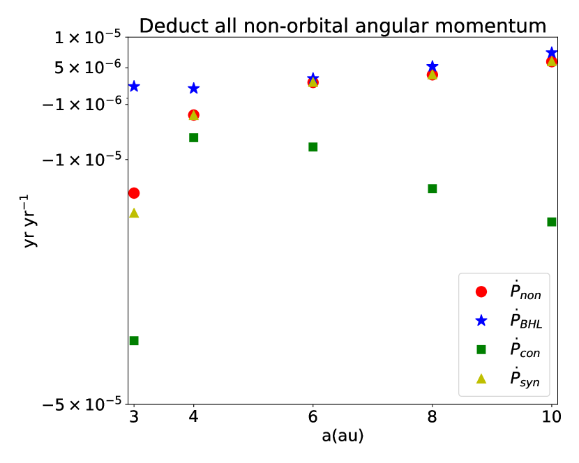
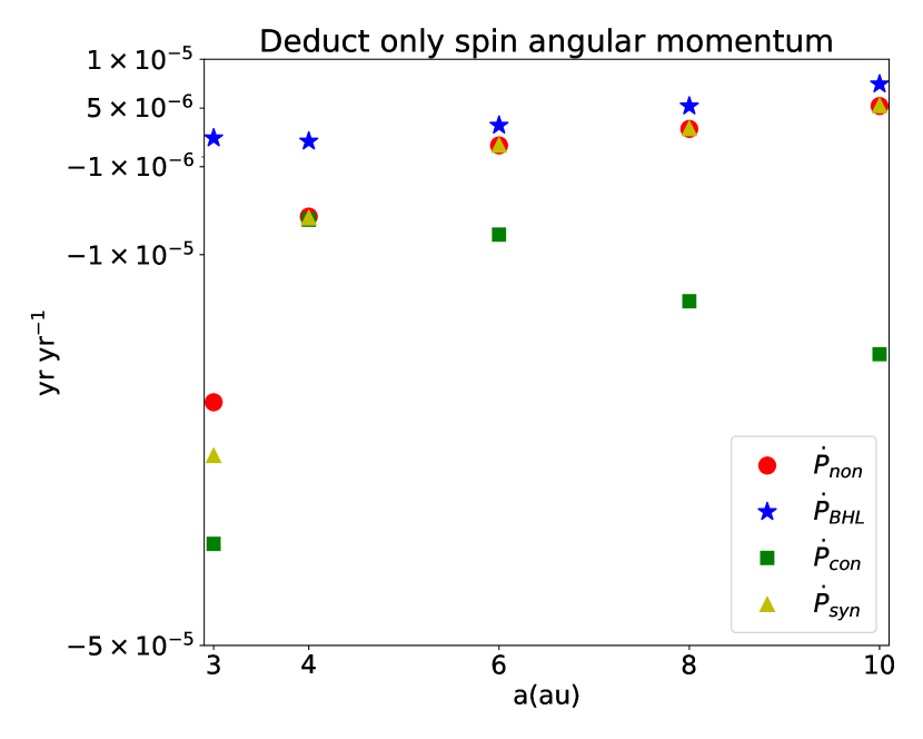
Figure 1: The first figure shows $\dot{P}_{\text{syn,exall}}$ and $\dot{P}_{\text{non,exall}}$ for our five binary models vs. their initial orbital separation. The second figure shows the corresponding plot for $\dot{P}_{\text{syn,exspin}}$ and $\dot{P}_{\text{non,exspin}}$. $\dot{P}_{\text{BHL}}$ and $\dot{P}_{\text{con}}$ are calculated from our analytic model. Their exact values can be found in Table 5.

As identified from Table 5 and Figure 1, two factors are most important: binary separation $a$ and the presence or absence of synchronization. We discuss each in turn.

In our 3D simulations, the AGB wind is standardized and so the binary separation $a$ will determine the mass transfer mode for a fixed secondary mass. The binary stars of models 1-3 are likely experiencing WRLOF while those of models 4 and 5 are likely experiencing BHL mass transfer. The orbital period change rates $\dot{P}_{\text{non}}$ and $\dot{P}_{\text{syn}}$ approach $\dot{P}_{\text{con}}$ for small binary separation but approaches $\dot{P}_{\text{BHL}}$ for large separation (Figure 1). The trend is monotonic since $\dot{P}_{\text{non}}$ and $\dot{P}_{\text{syn}}$ both increase with $a$. The orbital period decay (Table 5) occurs rapidly fast enough in models 1 and model 2 that they will incur RLOF or precursor (Darwin) instabilities (Lai et al., 1994) within the lifetime of the AGB star ($\sim 10^{6}$yr). They will ultimately incur a CE phase when the companion dives into the AGB envelope.

The AGB wind provides the driving force that changes the orbital period is the AGB wind. In its absense, there is no way to couple spin and orbital angular momenta. Without a wind $\dot{J}=\dot{m}_{1}=\dot{m}_{2}=0$ giving $\dot{a}=0$ and $\dot{P}=0$ and there will be no difference in orbital evolution for synchronized and initially non-spinning models. Comparing $\dot{P}_{\text{syn,exspin}}$ to $\dot{P}_{\text{non,exspin}}$ and $\dot{P}_{\text{syn,exall}}$ to $\dot{P}_{\text{non,exall}}$, we see that if $\dot{P}$ is negative, the synchronization makes it more negative. If $\dot{P}$ is positive, synchronization makes it more positive. This can be understood if we view the rotating giant star as a reservoir of angular momentum that extracts from the orbit when the binary stars orbit faster and releases to the orbit when the orbit is slower. Via the wind, the spin-orbit synchronization of the giant star can thus accelerate tightening or looseing of the orbit, the effect being stronger for closer binaries.

The wind speed also has some influence on the rate of orbital shrinking. Faster winds have less time to interact with the companion, thereby reducing angular momentum and mass transfer and increasing mass loss. From our isolated AGB star model (Chen et al., 2017), the terminal wind speed is $15$km s^-1 and the mass-loss rate is $2.31\times 10^{-7}$ M_⊙ yr^-1. Some AGB stars may eject slower winds ($5-10$km s^-1) with higher mass-loss rates ($\sim 10^{-6}$ M_⊙ yr^-1) (Freytag et al., 2017). In those cases, the binary system will be more likely to incur WRLOF the orbit will decay faster.

5 Astrophysical implications

A most interesting consequence of our analysis is the implications for orbital period decay, which in turn leads strongly interacting binaries (Nordhaus & Blackman, 2006; Ivanova & Nandez, 2016; Staff et al., 2016) such as CE and tidal disruption. From Table 5 (and also Figure 1), we conclude that $\dot{P}$ is a highly non-linear function of $a$ but smaller $a$ leads to faster OPD. The non-linearity is ascribed to the mode of mass transfer. Models 4 and 5 have BHL accretion which leads to relatively less interaction between the AGB wind and the secondary compared to WRLOF or RLOF. In contrast, models 1, 2 and 3 have WRLOF which is a more effective mass transfer mechanism than BHL accretion. As such, the gas in the can gain more angular momentum from the secondary and escape from the L2 point. When leaving the system, the gas carries a large fraction of angular momentum with a small fraction of mass of the binary as shown with $\gamma$ in Table 1.

As $\dot{a}$ increases monotonically with $a$ from negative to positive (Table 5), we can identify two key values $a_{\text{merge}}$ and $a_{\text{bi}}$. The former, $a_{\text{merge}}$, refers to the initial separation that distinguishes the binary systems that will and will not subsequently merge. The value $a_{\text{bi}}$ is the separation that distinguishes tightening from widening binaries. Specifically, in our simulation, $4$ au$<a_{\text{merge}}<a_{\text{bi}}<6$ au. The existence of such a boundary was previously inferred from a tidally interacting and BHL accretion binary model (Villaver & Livio, 2009; Nordhaus et al., 2010) and likely exists for any low mass ratio two-body system.

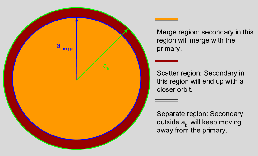
Figure 2: Conceptual fate of the secondary considering wind and tide.

The fate of the secondary is summarized in Fig. 2. The primary is located at the concentric center of these spheres. The orange color indicates the merge region. A secondary in this region will move towards the primary due to OPD and incur CE. Red indicates the scatter region. This region is identified by $a_{\text{merge}}$ and $a_{\text{bi}}$. The secondary in this region will experience OPD but the OPD is not strong enough for merging to happen during the AGB lifetime. At the end of the AGB evolution, the position of the secondary will then be scattered within $a_{\text{bi}}$.

Now we consider an ensemble of binary systems with secondaries distributed uniformly only in the scatter region i.e.

$$\rho(a,t_{\text{i}})=C$$ (20)

where $\rho$ is of being initially at binary separation $D(t_{\text{i}})=a$, where $a_{\text{merge}}<a<a_{\text{bi}}$ at initial time $t_{\text{i}}$. Here $C$ is a constant to normalize the probability integral. Since $\dot{P}$ decreases rapidly with evolving $D$, when the binary system evolves to its final state at $t_{\text{f}}$, the closer the secondary is to the WD, the smaller the probability $\rho(D,t_{\text{f}})$. We illustrate $\rho(a,t_{\text{i}})$ and $\rho(a,t_{\text{f}})$ conceptually in Fig. 3.

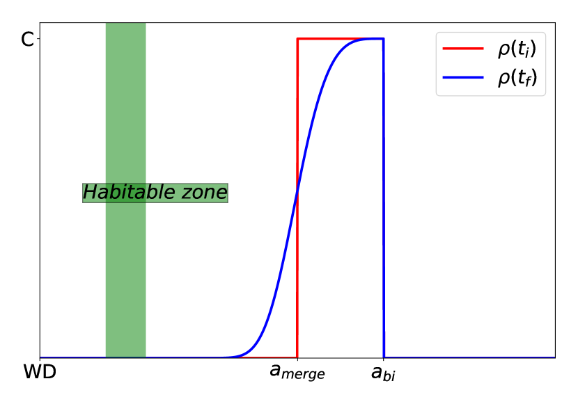
Figure 3: Conceptual $\rho(a,t_{\text{i}})$ and $\rho(a,t_{f})$. Green band represents the potential habitable zone and the WD is at the origin.

Although not simulated directly, our analytic model, along with the three regions of Figure 2, also speaks to the question of finding potential planets around WDs (Nordhaus & Spiegel, 2013) and particularly, in the habitable zone. Surviving planets must be in the scatter region about the primary in order to migrate close enough but avoid CE, wherein it would be destroyed (Nordhaus & Spiegel, 2013). However, this safety region is just thin shell of radial extent $<2$ au. Furthermore, $a_{\text{merge}}$ is usually not so small in giant binary systems and the nonlinear evolution of $\dot{a}$ even if initially beyond the merge region, would further decrease the possibility of finding a close planet around WD. This strengthens the argument that first-generation planets in the white dwarf habitable zone are unlikely unless tertiary or multi-body interactions result in scattering to high-eccentricity orbits (Nordhaus & Spiegel, 2013). Subsequent damping to circular orbits via tidal friction may be possible, but would initially leave rocky planets as uninhabitable, charred embers (Nordhaus & Spiegel, 2013).

6 Conclusions

We have studied the orbital period evolution in binary systems with a wind-emitting giant star, taking into account different modes (WRLOF and BHL accretion) of mass transfer ($\dot{m}_{2}$), mass loss ($\dot{m}_{1}$) and angular-momentum loss ($\dot{J}$). The time derivative of orbital separation $\dot{a}$ and that of the period $\dot{P}$ can be calculated analytically given $\dot{m}_{1},\dot{m}_{2}$ and $\dot{J}$. We have examined the validity if the giant star in our binary models can be synchronized under tidal force in Appendix A and considered both spin-orbit synchronized and zero spin AGB star scenarios.

We find that giant stars in close binary systems that undergo WRLOF are likely to be synchronized. We expect such systems to incur OPD and orbit decay to the point that RLOF or Darwin instabilities drive the system to a CE phase. Because WRLOF can happen at larger radii than RLOF or Darwin instabilities,the rapid evolution we find from the WRLOF phase implies an dramatic increase in the fraction of binaries that will arrive at CE were this phase ignored. In contrast, we find that wide binaries undergo BHL mass transfer and are likely to be separating. In this case a synchronized giant star could serve as an angular momentum reservoir that further enhances the separation.

We have identified two characteristic binary separations $a_{\text{merge}}$ and $a_{\text{bi}}$: $a_{\text{merge}}$ is the initial critical separation below with binaries merge and $a_{\text{bi}}$ is the critical separation at which $\dot{a}=0$. These two separations divide the space into three regions (Fig. 2): merge, scatter, and separate.

Angular-momentum loss ($\dot{J}$) and mass loss ($\dot{m}_{\text{esc}}$) are two competing factors in our model, just as tidal friction, drag force and mass loss are in Villaver & Livio (2009); Nordhaus & Spiegel (2013). All of these models agree that smaller separations lead to faster OPD although the mechanisms studied are different.

Finally, we emphasize the importance of 3D binary simulations for capturing the nonlinear evolution of the binary separation. In general, binary separation, mass of the stars and wind properties determine the mass transfer mode (RLOF, WRLOF, or BHL) and interaction (tides and instabilities). As binary stars get closer, the more a self-consistent giant star model is needed to resolve the fluid motion and stellar structure. The dynamical evolution between mass transfer modes is warrants 3D binary simulations. Crudely assuming only BHL accretion, for example, without following the nonlinear evolution of the accretion mode can miss the rapid OPD and subsequent merger if the actual system evolves to WRLOF when the separation decreases.

Appendix A Justifying Spin-Orbit Synchronized AGB star

In our 3D simulations, the boundary condition of the AGB star we used is in spin-orbit synchronized state. However, the AGB stellar spin may not be synchronized in widely separated binaries with small mass ratios. To justify the assumption of synchronization, we calculate the synchronization timescale for the giant star using equation (5) in Nordhaus & Spiegel (2013). If the timescale is much shorter than the lifetime of the AGB star and the timescale for the binary to merge, then the synchronized boundary condition can be justified. The time-evolution of the spin is given by

$$\left(\frac{\text{d}\Omega_{1}}{\text{d}t}\right)_{\text{tides}}=\frac{6\omega k_{2,1}f}{\alpha_{1}\tau_{1,\text{conv}}}\left(\frac{m_{1,\text{env}}}{m_{1}}\right)\left(\frac{m_{2}}{m_{1}}\right)^{2}\left(\frac{R_{1}}{a}\right)^{6}\left(1-\frac{\Omega_{1}}{\omega}\right)-\Omega_{1}\frac{\dot{I}_{1}}{I_{1}}$$ (21)

where $\omega,\Omega_{1},R_{1},m_{1},m_{1,\text{env}},I_{1}$ are the circular orbital angular frequency of the binary system, rotational angular frequency, radius, total mass, envelop mass and moment of inertia of the giant star, $m_{2}$ is the total mass of the secondary, $\tau_{1,\text{conv}}=\left(m_{1,\text{env}}R_{1}^{2}/L_{1}\right)^{1/3}$ and $L_{1}$ is the luminosity of the giant star. The tidal Love number of the giant is $k_{2,1}$ which we assume to be unity, $f$ is also close to unity (Nordhaus & Spiegel, 2013). For a spherically symmetric density distribution, the moment of inertia is calculated by:

$$I=\int_{0}^{R}\frac{8\pi r^{4}\rho(r)}{3}\text{d}r=\alpha mR^{2}$$ (22)

where $\alpha,R$ and $m$ are the moment of inertia factor, radius of the sphere (star) and the total mass of the star, respectively. In an evolving star, $I,\alpha,R$ and $m$ will all be time dependent variables. However, for simplicity, we only consider the time dependence of $I$ and $m$ in this paper and assume $\alpha$ and $R$ to be constant in a short period of time. The time scale for the giant star to be synchronized is then estimated by:

$$t=\frac{\omega}{\text{d}\Omega/\text{d}t}$$ (23)

taking $\Omega(t=0)=0$.

The remaining parameters needed to calculate $\text{d}\Omega/\text{d}t$ are: $\alpha,m_{1,\text{env}},R_{1}$ and $L_{1}$. MESA (Modules for Experiments in Stellar Astrophysics) (Paxton et al., 2015) can provide us the values. We take a 1.3 M_⊙ ZAMS as an illustrative example. When it evolves to 1 M_⊙, $\alpha\approx 0.063$, $m_{\text{env}}\approx 0.45\text{M}_{\sun}$, $R_{1}\approx 0.9\text{au}$ and $L\approx 3100\text{L}_{\sun}$. We notice that the luminosity predicted by MESA is greater than the luminosity ($2342\text{L}_{\sun}$) we used in our 3D simulation. However, our AGB star model is a phenomenological model and we focus on the wind structure instead of the core and the envelope of the star. Our model has produced an AGB wind with reasonable speed ($\sim 15\text{km/s}$) and a lower density. We view the discrepancy as a potential challenge and opportunity for future studies. To estimate the timescale (table 6) of synchronization, we use the values from MESA.

From the resulting calculation, we find that the timescale to synchronize the giant star is much smaller than the lifetime of the AGB star ($\sim 10^{6}$yr) and the timescale to merge ($10^{5}-10^{6}$yr) (perhaps except for model 5) as we see in the calculations of section 4.4). Therefore, we find it reasonable to assume that the AGB star should be synchronized throughout the simulations for models 1-3. On the other hand, we discuss and the non-synchronized nature of model 5 in more detail and give the corrected answer. The giant star in model 4 is likely partially synchronized.

model	$m_{1}$	$m_{2}$	$a$	$t$
	M☉	M☉	au	yr
1	1.0	0.1	3	2.41$\times 10^{3}$
2	1.0	0.5	4	5.42$\times 10^{2}$
3	1.0	0.5	6	6.17$\times 10^{3}$
4	1.0	0.5	8	3.47$\times 10^{4}$
5	1.0	0.5	10	1.32$\times 10^{5}$

Table 6: The first column lists the model number used throughout this paper; $m_{1}$ and $m_{2}$ are the mass of the giant star and the secondary, respectively; $a(\text{au})$ is the binary separation; $t$ is the synchronization timescale of the giant star.

As the binary separation is decreasing in model 1 and model 2, the synchronization assumption can hold for future long-term evolution (Perhaps model 3 also as the two stars are not separating fast). We will discuss the non-synchronous scenario in Section 4.4.

Appendix B angular momentum error in AGB wind

In this section, we quantify the angular momentum error (’the error’ hereafter) in our isolated AGB wind model. Ideally, when supersonic fluid is moving outward in a central potential (a combination of gravitational force and radiation force), its angular momentum should not change ($\dot{J}=$const.). In our model, gas will become supersonic when dust forms.

Since we have five binary models, each with different binary orbital angular frequencies, we examine the error of an isolated AGB wind for different angular frequencies. Each simulation has an AGB star at the center of the simulation box. The simulation is also carried out in co-rotating frame, with $\omega=\sqrt{G(m_{1}+m_{2})/a^{3}}$. This should be equivalent to simulation of AGB star which spins at $\omega$ in lab-frame. We measure the average angular momentum flux $\dot{J}$ through sampling shells (centered at the center of the AGB star) at a series of radii $[0.8a,0.9a,1.0a,1.1a,1.2a,1.3a,1.4a]$. $a$ is the binary separation.

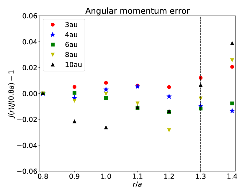
Figure 4: Angular momentum error in AGB wind. The x-axis is the distance in binary separation. The y-axis is the value of error. Five different makers show the error of corresponding angular frequency of the binary model with that separation. The vertical dotted line denote the radius of sampling shell that we use in parameter measurement (Section 4.1).

We plot the error of different models in Figure 4. We can see that the error in AGB wind is acceptable, or within $4\%$ of all the angular momentum in the AGB wind.

Appendix C time varying $\gamma$

The AGB binary models in this paper take dust formation, radiation transfer and cooling into consideration and thus the system is highly dynamic, especially when there is a large accretion disc. We note that Eulerian codes in Cartesian coordinates are generally poor at conserving angular momentum at large amid the coarse grid. We thus we measure the angular momentum flux at relatively small radii $r_{\text{flux}}=1.3a$. The AMR capability of ASTROBEAR can help us resolve the central part of the binary system and thus minimize the error.

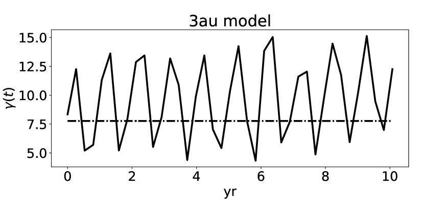
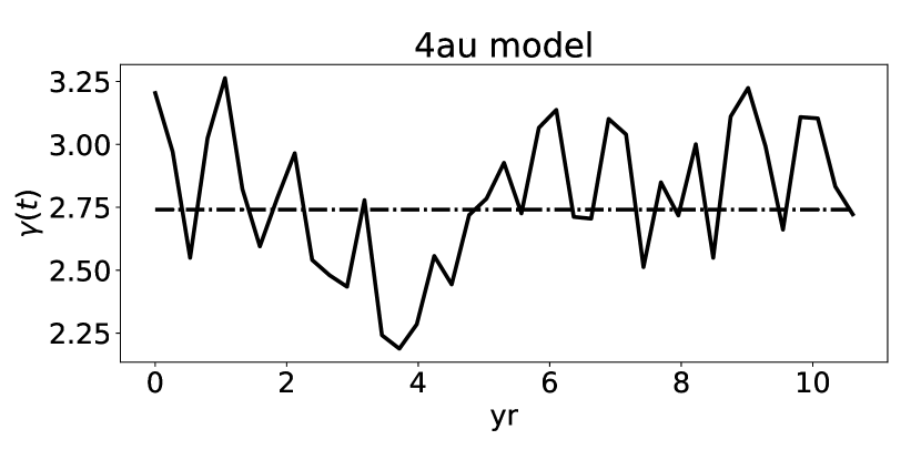
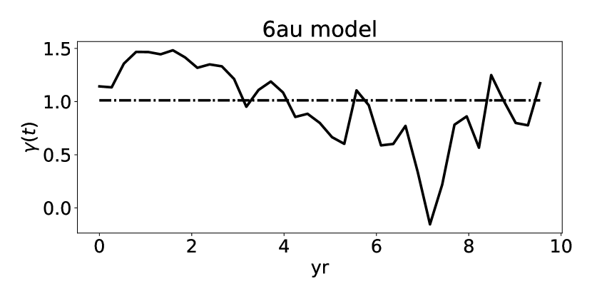
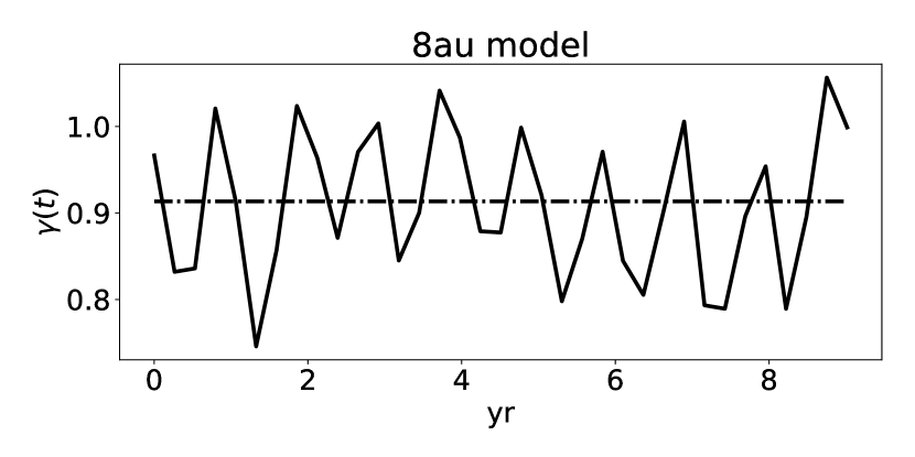
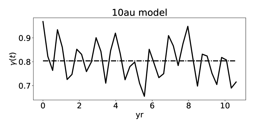
Figure 5: The solid lines show the sampled time varying $\gamma(t)$ of our five binary models. The dashed lines are the averaged $\gamma$.

Fig. 5 shows the time varying $\gamma(t)$ and averaged $\gamma$ of each models. There is a $1$yr period in $\gamma(t)$ corresponding to the AGB pulsation. We also notice that there are dips in the $4$au and $6$au models but not in other models. We infer these to be waves in the accretion disc and fall back. Both $4$au and $6$au simulations have large accretion discs (see Fig. 4 in Chen et al. (2017)). Since the sampling shell is at $r_{\text{flux}}$, the waves in the accretion disc and also in the circumbinary disc can propagate to the sampling shell. However, we do not have a self-consistent model of these waves (see discussions in Sec. 2.3 in Chen et al. (2017)) for the accretion disc and view this problem as a future research direction.

References

- Akashi et al. (2015) Akashi M., Sabach E., Yogev O., Soker N., 2015, MNRAS, 453, 2115
- Balick & Frank (2002) Balick B., Frank A., 2002, ARA&A, 40, 439
- Bear & Soker (2017) Bear E., Soker N., 2017, ApJ, 837, L10
- Bond et al. (2003) Bond H. E., et al., 2003, Nature, 422, 405
- Bondi & Hoyle (1944) Bondi H., Hoyle F., 1944, MNRAS, 104, 273
- Boyarchuk et al. (2002) Boyarchuk A. A., Bisikalo D. V., Kuznetsov O. A., Chechetkin V. M., 2002, Mass transfer in close binary stars
- Brown et al. (2002) Brown N. J., Waagen E. O., Scovil C., Nelson P., Oksanen A., Solonen J., Price A., 2002, IAU Circ., 7785
- Carroll-Nellenback et al. (2013) Carroll-Nellenback J. J., Shroyer B., Frank A., Ding C., 2013, Journal of Computational Physics, 236, 461
- Chen et al. (2017) Chen Z., Frank A., Blackman E. G., Nordhaus J., Carroll-Nellenback J., 2017, MNRAS, 468, 4465
- Cunningham et al. (2009) Cunningham A. J., Frank A., Varnière P., Mitran S., Jones T. W., 2009, ApJS, 182, 519
- Edgar (2004) Edgar R., 2004, New Astron. Rev., 48, 843
- Freytag et al. (2017) Freytag B., Liljegren S., Höfner S., 2017, A&A, 600, A137
- Han et al. (1995) Han Z., Podsiadlowski P., Eggleton P. P., 1995, MNRAS, 272, 800
- Hillwig et al. (2016) Hillwig T. C., Jones D., De Marco O., Bond H. E., Margheim S., Frew D., 2016, ApJ, 832, 125
- Hoyle & Lyttleton (1939) Hoyle F., Lyttleton R. A., 1939, Proceedings of the Cambridge Philosophical Society, 35, 405
- Iben & Tutukov (1984) Iben Jr. I., Tutukov A. V., 1984, ApJS, 54, 335
- Ivanova & Nandez (2016) Ivanova N., Nandez J. L. A., 2016, MNRAS, 462, 362
- Ivanova et al. (2013) Ivanova N., et al., 2013, A&ARv, 21, 59
- Kenyon et al. (1993) Kenyon S. J., Livio M., Mikolajewska J., Tout C. A., 1993, ApJ, 407, L81
- Kervella et al. (2016) Kervella P., Homan W., Richards A., Decin L., McDonald I., Montargès M., Ohnaka K., 2016, Astronomy & Astrophysics
- Kim et al. (2017) Kim H., Trejo A., Liu S.-Y., Sahai R., Taam R. E., Morris M. R., Hirano N., Hsieh I.-T., 2017, Nature Astronomy, 1, 0060
- Krumholz et al. (2004) Krumholz M. R., McKee C. F., Klein R. I., 2004, ApJ, 611, 399
- Kulkarni et al. (2007) Kulkarni S. R., et al., 2007, Nature, 447, 458
- Lai et al. (1994) Lai D., Rasio F. A., Shapiro S. L., 1994, ApJ, 423, 344
- Lin (1977) Lin D. N. C., 1977, MNRAS, 179, 265
- MacFadyen & Milosavljević (2008) MacFadyen A. I., Milosavljević M., 2008, ApJ, 672, 83
- MacLeod et al. (2017) MacLeod M., Macias P., Ramirez-Ruiz E., Grindlay J., Batta A., Montes G., 2017, ApJ, 835, 282
- Maercker et al. (2012) Maercker M., et al., 2012, Nature, 490, 232
- Martini et al. (1999) Martini P., Wagner R. M., Tomaney A., Rich R. M., della Valle M., Hauschildt P. H., 1999, AJ, 118, 1034
- Mastrodemos & Morris (1998) Mastrodemos N., Morris M., 1998, ApJ, 497, 303
- Metzger & Pejcha (2017) Metzger B. D., Pejcha O., 2017, preprint, (arXiv:1705.03895)
- Miszalski et al. (2017) Miszalski B., Manick R., Mikołajewska J., Iłkiewicz K., Kamath D., Van Winckel H., 2017, preprint, (arXiv:1703.10891)
- Munari et al. (2005) Munari U., et al., 2005, A&A, 434, 1107
- Nordhaus & Blackman (2006) Nordhaus J., Blackman E. G., 2006, MNRAS, 370, 2004
- Nordhaus & Spiegel (2013) Nordhaus J., Spiegel D. S., 2013, MNRAS, 432, 500
- Nordhaus et al. (2007) Nordhaus J., Blackman E. G., Frank A., 2007, MNRAS, 376, 599
- Nordhaus et al. (2010) Nordhaus J., Spiegel D. S., Ibgui L., Goodman J., Burrows A., 2010, MNRAS, 408, 631
- Nordhaus et al. (2011) Nordhaus J., Wellons S., Spiegel D. S., Metzger B. D., Blackman E. G., 2011, Proceedings of the National Academy of Science, 108, 3135
- Paczyński (1971) Paczyński B., 1971, ARA&A, 9, 183
- Paxton et al. (2015) Paxton B., et al., 2015, ApJS, 220, 15
- Pejcha et al. (2016) Pejcha O., Metzger B. D., Tomida K., 2016, MNRAS, 455, 4351
- Podsiadlowski & Mohamed (2007) Podsiadlowski P., Mohamed S., 2007, Baltic Astronomy, 16, 26
- Pribulla (1998) Pribulla T., 1998, Contributions of the Astronomical Observatory Skalnate Pleso, 28, 101
- Rau et al. (2007) Rau A., Kulkarni S. R., Ofek E. O., Yan L., 2007, ApJ, 659, 1536
- Rich et al. (1989) Rich R. M., Mould J., Picard A., Frogel J. A., Davies R., 1989, ApJ, 341, L51
- Santander-García et al. (2015) Santander-García M., Rodríguez-Gil P., Corradi R. L. M., Jones D., Miszalski B., Boffin H. M. J., Rubio-Díez M. M., Kotze M. M., 2015, Nature, 519, 63
- Soker & Livio (1994) Soker N., Livio M., 1994, ApJ, 421, 219
- Springel et al. (2005) Springel V., Di Matteo T., Hernquist L., 2005, MNRAS, 361, 776
- Staff et al. (2016) Staff J. E., De Marco O., Wood P., Galaviz P., Passy J.-C., 2016, MNRAS, 458, 832
- Tout & Hall (1991) Tout C. A., Hall D. S., 1991, MNRAS, 253, 9
- Tylenda (2005) Tylenda R., 2005, A&A, 436, 1009
- Tylenda et al. (2011) Tylenda R., et al., 2011, A&A, 528, A114
- Villaver & Livio (2009) Villaver E., Livio M., 2009, ApJ, 705, L81
- Zahn (1977) Zahn J.-P., 1977, A&A, 57, 383
- Zahn (1989) Zahn J.-P., 1989, A&A, 220, 112