Multiwavelength monitoring of a very active dwarf nova AX J1549.8$-$5416 with an unusually high duty cycle

Abstract

We present the results of our analysis of new optical, ultraviolet (UV) and X-ray observations of a highly variable source $-$ AX J1549.8–5416. Both the detection of several fast rise, exponential decay outbursts in the optical light curve and the lack of He II emission lines in the optical spectra suggest AX J1549.8–5416 is a cataclysmic variable of the dwarf nova (DN) type. The multiwavelength analysis of three mini-outbursts and one normal outburst represent one of the most complete multiwavelength studies of a DN and help to refine the relationship between the X-ray, UV and optical emission in this system. We find that the UV emission is delayed with respect to the optical by $1.0-5.4$ days during the rising phase of the outburst. The X-ray emission is suppressed during the peak of the optical outburst and recovers during the end of the outburst. From our analysis of archival Swift, Chandra and XMM-Newton observations of AX J1549.8–5416, we estimate this DN has a high duty cycle ($\sim 50\%$), suggesting a quiescent X-ray luminosity larger than $10^{32}$ erg/s. We also find the X-ray and UV flux are roughly anti-correlated. Furthermore, we find that, at low X-ray fluxes, the X-ray spectrum is well described by a single temperature thermal plasma model, while at high X-ray fluxes, an isobaric cooling flow model also works. We find that the maximum temperature of the plasma in quiescence is significantly higher than that in outburst.

1 introduction

Cataclysmic variables (CVs) are interacting binaries consisting of a low-mass secondary star very close to a more massive white dwarf (WD) primary star. The WD accretes matter from the companion star via Roche lobe overflow. CVs are classified into several types based on their observational characteristics, depending on the nature of the primary star and the accretion process (see reviews by Kuulkers et al., 2006; Singh, 2013). In particular, CVs are divided into non-magnetic CVs (non-MCVs) and magnetic CVs (MCVs) based on the strength of the WD surface magnetic field. In non-MCVs, X-rays are thought to originate from the boundary layer (BL) between the slowly rotating accreting WD and the fast rotating (Keplerian) inner edge of the accretion disc, where the material dissipates its remaining rotational kinetic energy before accreting onto the surface of the WD. In MCVs, X-rays originate from an accretion column at or near the magnetic poles. The columns may be fed via magnetospheric accretion from the inner boundary of a truncated disc, as in the subclass of intermediate polars (IPs), or from a funneled accretion stream in polars. The X-ray spectra of magnetic and non-magnetic CVs are typically described by multi-temperature thermal plasma emission (e.g., Kuulkers et al., 2006; Singh, 2013).

Dwarf novae (DNe) are non-MCVs with an accretion disc that flows onto the WD primary, and a secondary star. The orbital periods of DNe are typically between 70 minutes and 10 hours (Kuulkers et al., 2006; Patterson, 2011; Balman, 2012). In DNe, the accretion disc has two stable states which correspond to optical quiescence and outbursts. During optical quiescence, the X-ray emission arises from the hot, optically thin, thermal plasma produced at the BL. The X-ray spectrum is hard, has a temperature greater than 10 keV, and typically features associated with the Fe K_α line are observed. Furthermore, during this state the optically thick accretion disc is truncated, and the accretion rate is less than $10^{-9}-10^{-9.5}$ $\mathrm{M}_{\odot}$/year.

When in outburst, the optical flux increases by 2$-$9 magnitudes for several days to weeks. This increase is associated with an increase in the luminosity of the accretion disc which dominates the emission at optical and UV wavelengths (e.g., Lasota, 2001; Kuulkers et al., 2006). During this period, the X-ray spectra is soft, and the plasma temperature decreases such that the thermal emission peaks in the extreme UV. Due to the increase in accretion rate on the WD, the plasma in the BL becomes optically thick and therefore more efficient at cooling (Pandel et al., 2003; Saitou et al., 2012; Baskill et al., 2005; Collins & Wheatley, 2010; McGowan et al., 2004). The mechanism leading to repeated transitions between the optical outburst and quiescent states is thought to be thermal viscous disc instability (e.g., Meyer & Meyer-Hofmeister, 1981; Lasota, 2001).

An analysis of archival Swift  data identified a highly variable X-ray source – AX J1549.8–5416 – which was first detected in the ASCA Galactic plane Survey (Sugizaki et al., 2001). Its optical counterpart was proposed to be NSV 20407, a variable star with a B-band magnitude ranging from $>18$ to 16.7 (Samus et al., 2009), suggesting this source is a CV. Lin et al. (2014) analysed four XMM-Newton observations of AX J1549.8–5416 and found that the source’s X-ray flux varied considerably. They also detected a Fe line in the X-ray spectra of two observations and suggested this source be a MCV, which often have Fe emission in their X-ray spectra (Ezuka & Ishida, 1999).

In order to further investigate the nature of AX J1549.8–5416, we observed the source at optical wavelengths with the Las Cumbres Observatory Global Telescope Network (LCOGT) and ’Jorge Sahade’ at CASLEO (Argentina), complemented with UV and X-ray observations by Swift. Since AX J1549.8–5416 is located $\sim 9.2$ arcmin away from 1E 1547.0$-$5408, it is within the field of view of a large number of archival Swift observations. In this paper, we also analysed all available archival XMM-Newton, Chandra, and Swift data of the source. We describe the observations and data reduction in Section 2, and we present our results in Section 3. Finally, in Section 4 we discuss our findings and summarize our conclusions in Section 5.

2 Observations and data reduction

2.1 LCOGT Optical observations

We observed the field of AX J1549.8–5416 with the LCOGT suite of robotic 1-m telescopes, from 2015-04-30 to 2015-06-18 and from 2016-02-01 to 2016-04-30. Some data in 2016 were taken with the 2-m Faulkes Telescope South (FTS). These data were acquired as part of our Faulkes Telescopes monitoring project of X-ray transients (Lewis et al., 2008). Optical images were acquired in four filters: Bessel $B$-band, $V$-band, $R$-band and SDSS $i^{\prime}$-band. The observation logs are provided in Table 7. All LCOGT telescopes are equipped with a camera with pixel scale 0.467 arcsec pixel^-1, while the camera of FTS has 0.301 arcsec pixel^-1. Bias subtraction and flat-fielding were performed via the automatic pipelines.

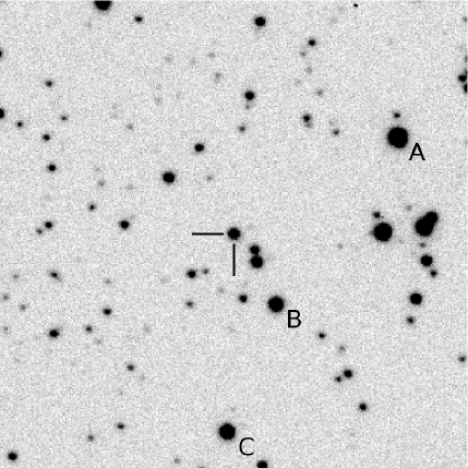
Figure 1: Optical ($R$-band, taken on 2015-06-10 at Cerro Tololo) finding chart. The field of view is 3.0 $\times$ 3.0 arcmin; north is up and east is to the left. AX J1549.8–5416 is marked at the centre, and the stars A, B and C are the three used for flux calibration.

The optical counterpart of AX J1549.8–5416 is clearly visible, at a location consistent with the position of the X-ray source, the UV source and the known variable star NSV 20407. Photometry was performed on the target and three field stars in the APASS data release 9 catalogue (Henden et al., 2015, see Fig. 1) using PHOT in IRAF, adopting a 2.8 arcsec aperture. We calibrated the field using the catalogue $B$, $V$ and $i^{\prime}$-band magnitudes of the three field stars, which have typical errors of 0.01–0.1 mag. $R$-band flux calibration was achieved using the transformation from $V$, $r^{\prime}$ and $i^{\prime}$-bands described by Jordi et al. (2006).

Table 1: New Swift/XRT observations. The error bars are given in 1-$\sigma$ level.

ObsID	Date UT	MJD	exposure (s)	X-ray rate ($\times 10^{-3}$cnt/s)	UV magnitude	UVOT filter
00042706002	2016-02-11T17:40:32	57429.73648148	685	6.09 $\pm$ 3.04	$>$ 20.3	uvw2
00042706003	2016-02-15T22:14:32	57433.92675926	505	4.19 $\pm$ 2.96	19.37 $\pm$ 0.2	uvw2
00042706004	2016-02-19T15:25:11	57437.64248843	585	31.61 $\pm$ 7.45	19.31 $\pm$ 0.18	uvw2
00042706005	2016-02-24T22:58:47	57442.95748843	850	16.94 $\pm$ 4.52	19.22 $\pm$ 0.18	uvm2
00042706006	2016-02-27T11:48:53	57445.49228009	775	13.17 $\pm$ 4.16	20.04 $\pm$ 0.29	uvw2
00042706007	2016-03-04T04:42:00	57451.19583333	1135	7.19 $\pm$ 2.54	19.11 $\pm$ 0.12	uvw1
00042706008	2016-03-14T20:13:22	57461.84322042	995	3.08 $\pm$ 1.78	19.21 $\pm$ 0.13	uvw2
00042706009	2016-03-18T04:11:02	57465.17493410	810	1.25 $\pm$ 1.25	18.89 $\pm$ 0.13	uvw2
00042706010	2016-03-25T08:07:36	57472.33861111	1020	13.11 $\pm$ 3.63	18.50 $\pm$ 0.15	u
00042706011	2016-03-28T01:36:03	57475.06670139	895	11.31 $\pm$ 3.57	19.04 $\pm$ 0.14	uvw1
00042706012	2016-03-31T21:52:52	57478.91171296	965	22.07 $\pm$ 4.81	$>$ 20.28	uvm2
00042706013	2016-04-03T01:12:19	57481.05021991	1000	19.41 $\pm$ 4.45	$>$ 20.37	uvw2
00042706014	2016-04-06T12:13:08	57484.50912037	890	6.92 $\pm$ 2.82	$>$ 20.41	u)
00042706015	2016-04-09T10:27:51	57487.43600694	485	2.07 $\pm$ 1.99	16.33 $\pm$ 0.04	uvw1
00042706016	2016-04-10T19:56:28	57488.83167344	472	6.35 $\pm$ 3.67	15.82 $\pm$ 0.03	u
00042706016	—	—	—	—	16.88 $\pm$ 0.09	uvw2
00042706017	2016-04-16T22:34:05	57494.94112905	830	—	17.94 $\pm$ 0.08	uvm2
00042706018	2016-04-19T22:27:44	57497.93672437	945	—	18.85 $\pm$ 0.20	uvw2
00042706019	2016-04-22T08:58:27	57500.37471492	904	9.60 $\pm$ 3.32	18.17 $\pm$ 0.06	u
00042706020	2016-04-25T23:17:06	57503.97099751	670	10.14 $\pm$ 3.95	19.86 $\pm$ 0.29	uvw1

For the first four observations, all four filters were used to constrain the colour and variability amplitude of the source. Variations of amplitude $\sim 2$ mag were seen in all bands, and for subsequent observations just $R$-band was used (see Table 7 for details). As a check of our relative errors, photometry was performed on a fourth field star in $R$-band. Its magnitude differed from its mean value of $R=16.11$ mag by $<2\sigma$ in 25 of 26 images in 2015. The mean error on the magnitude of this field star measured from each image was 0.03 mag, and for AX J1549.8–5416 the mean magnitude errors were 0.10, 0.05, 0.04 and 0.04 mag in $B$, $V$, $R$ and $i^{\prime}$-bands, respectively. The image quality was particularly bad in the observation taken on 2015-06-18, which resulted in a larger magnitude error. On 2015-06-10, 20 $R$-band images were taken to search for short-term variability. The results are shown in Section 3.1. In 2016 we carried out a high cadence monitoring campaign in R-band to closely follow the morphology and evolution of a full outburst.

2.2 CASLEO optical observations

Optical spectra of NSV 20407, the optical counterpart of AX J1549.8–5416, were acquired using the 2.15-m ’Jorge Sahade’ telescope at CASLEO (Argentina). This telescope is equipped with a REOSC spectrograph, which carries a 1024$\times$1024 pixel TEK CCD. The spectra were acquired in Simple Dispersion mode using the #270 grism (300 lines/mm) and a 2^′′ slit width, allowing one to nominally cover the 3500$-$7500 Å spectral range with a dispersion of 3.4 Å pixel^-1.

Two 1200-s spectroscopic frames were secured on 2015 April 14, with start times of 04:54 and 05:16 UT, respectively. After cosmic ray rejection, the spectra were reduced, background subtracted and extracted (Horne, 1986) using IRAF (Tody, 1993). Wavelength calibration was performed using Cu-Ne-Ar lamps acquired before each spectroscopic exposure; the spectra were then flux-calibrated using the spectrophotometric standard LTT 6284 (Hamuy et al. 1994). Finally, the two spectra were stacked together to increase the signal-to-noise ratio. The wavelength calibration uncertainty was $\sim$0.5 Å; this was checked using the positions of background night sky lines.

2.3 Swift observations

We analysed all available observations since 2007 June 2 (including archival and new observations that we requested), taken in Photon Counting (PC) mode with the X-Ray Telescope (XRT; Burrows et al., 2005) on board the Swift satellite. The XRT observations with exposure times longer than 500s were reduced using the Swift tools within the heasoft v. 6.16 (Blackburn, 1995) software package. Source detection and position determination were carried out using the recipes described in Evans et al. (2009). The source light curves and spectra were extracted in the 0.5$-$10.0 keV band using a circular extraction region with a radius of 20 arcsec centred on the position of the source. Background data were extracted from an annular region with an inner (outer) radius of 30 arcsec (60 arcsec). The 19 new Swift observations are shown in Table 1.

Since AX J1549.8–5416 is not at the center source of the archival Swift observations and the UVOT field of view is smaller than XRT, the source was not observed in all UVOT observations. We reduced all available UVOT observations which contained this source in the field. In each UVOT observation, this source was observed with at least one of the four filters with corresponding central wavelengths (Poole et al. 2008): uvw2 (1928 Å) uvm2 (2246 Å), uvw1 (2600Å), and u (3465Å). The UVOT data were analysed following the methods of Poole et al. (2008) and Brown et al. (2009).

2.4 XMM-Newton observations

Table 2: The XMM-Newton and Chandra observations in which the source was detected. The source net count rates were calculated in the 0.3–10 keV energy band converted using pimms. Errors represent the 90% confidence level. We converted the XMM-Newton and Chandra count rate to equivalent Swift-XRT count rates. The last column shows the 3-$\sigma$ upper limit of the pulsed fraction for each observation.

Instr.	No.	ObsID	Date	Exp.	Rate	Rate(XRT/PC)	pulsed fraction upper limit
				ks	$10^{-2}~{}\mathrm{counts~{}s}^{-1}$	$10^{-3}~{}\mathrm{counts~{}s}^{-1}$	%
XMM-Newton	1	0203910101	2004 Feb.	9.1	$11.3\pm 0.5$	9.34	6.2
Chandra	2	7287	2006 Jun	9.5	$3.21\pm 0.15$	4.71	6.5
XMM-Newton	3	0402910101	2006 Aug.	38.3	$5.86\pm 0.15$	4.91	6.1
XMM-Newton	4	0410581901	2007 Aug.	12.4	$0.41\pm 0.01$	0.39	6.6
XMM-Newton	5	0560181101	2009 Feb.	48.7	$3.70\pm 0.11$	3.11	6.5
XMM-Newton	6	0604880101	2010 Feb.	40.4	$0.54\pm 0.08$	0.52	5.4
Chandra	7	12554	2011 Jun	96.5	$0.78\pm 0.03$	1.12	5.8

We analysed five XMM-Newton observations of the source between February 2004 and February 2010. We reduced the XMM-Newton Observation Data Files (ODF) using version 12.0.1 of the Science Analysis Software (sas). We used the epproc task to extract the event files for the PN camera. Source light curves and spectra were extracted in the 0.5–10.0 keV band using a circular extraction region with a radius of 20 arcsec centred on the position of the source. Background light curves and spectra were extracted from a circular source-free region of radius 30 arcsec on the same CCD. We applied standard filtering and examined the light curves for background flares. Only Obsid 0402910101 contained flares and we used the non-flared exposures for our analysis. We checked the filtered event files for photon pile-up by running the task epatplot. No pile-up was apparent in the data. Photon redistribution matrices and ancillary files were created using the sas tools rmfgen and arfgen, respectively. We rebinned the source spectra using the tool grppha, such that the minimum number of counts per bin of the PN spectra was 25.

2.5 Chandra observations

We analysed two Chandra observations of AX J1549.8–5416 performed on Jun 2006 and Jun 2011, respectively (Table 2). We used the ciao tools (v. 4.5; Fruscione et al., 2006) and standard Chandra analysis threads to reduce the data. No background flares were found, so all data were used for further analysis.

The source spectra and light curves were extracted from a circular region with a radius of 20 arcsec centred on the position of AX J1549.8–5416. Background events were obtained from an annular region with an inner (outer) radius of 30 arcsec (60 arcsec). Using the ftool grppha, we re-binned the spectra to contain a minimum of 25 photons per bin.

3 Analysis and Results

3.1 Optical light curves

The top panel of Fig. 2 shows the optical light curve of AX J1549.8–5416 observed by LCOGT in April – June 2015. The source showed two clear outbursts within $\sim 40$ days, with the two peaks $\sim 35$ days apart. During the first outburst, the source was observed in $B$, $V$, $R$ and $i^{\prime}$-bands. During the second outburst, the source was observed in $R$-band only, with some higher time resolution ($\sim 2$ minutes) sequences on 2015 June 10. The lower panels of Fig. 2 show two zoom-in plots of the second peak. The source is less variable at short timescales (minutes) than at longer timescales ($\sim$10 days).

The general morphology of the outbursts is consistent with a fast rise, exponential decay (FRED; e.g. Chen et al., 1997), with the optical spectrum becoming bluer at higher fluxes. The rise rates between the first and second dates were 2.3, 2.2, 1.9 and 1.6 magnitudes in 5.26 days in $B$, $V$, $R$ and $i^{\prime}$-bands, respectively (0.44, 0.41, 0.36 and 0.31 mag/day). The rise rate of the second outburst was 2.2 mag in 3.3 days in $R$-band (0.65 mag/day), which may suggest the first outburst rise was quicker than measured since the first rise was not well sampled. The decay rates between the second and fourth dates (over 19.0 days) were 0.096, 0.088, 0.077 and 0.067 mag/day in $B$, $V$, $R$ and $i^{\prime}$-bands. The amplitude of the variations are larger at shorter wavelengths, which is expected for an accretion disc described by a simple blackbody that is hotter when it is brighter (this is also the case for low-mass X-ray binaries; see Maitra & Bailyn, 2008; Russell et al., 2011).

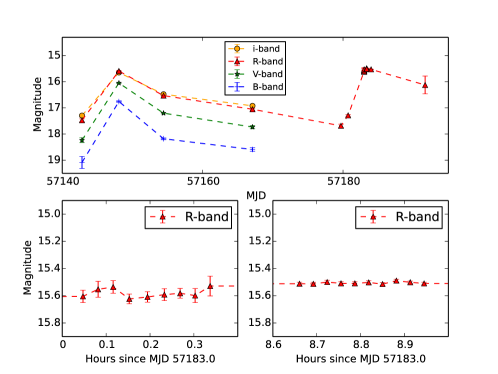
Figure 2: The optical light curve of the source in 2015. The top panel shows the optical light curve of AX J1549.8–5416 in i$\arcmin$, R, V and B band with orange, red, green and blue colour, respectively. The bottom panels show two zoom-in plots on the second peak with higher time resolution.

Serendipitously, our monitoring caught the fast rise of the next outburst, and the short time series coincided almost exactly with the peak of the outburst (Fig. 2). On 2015-06-10, the average magnitude was $R=15.58$ from data taken at 00:02–00:22 UT (9 consecutive images, at a time resolution of 131 sec), and $R=15.51$ at 08:39–08:58 UT. No intrinsic variability is detected; the magnitudes generally agreed within the errors of each measurement. The conditions were good during the second time series and worse during the first, with mean magnitude measurement errors of 0.048 mag at 00:02–00:22 UT and 0.012 mag at 08:39–08:58 UT. The fractional rms variability (calculated adopting the prescription described in Gandhi et al., 2010) was $<13.7$ per cent at 00:02–00:22 UT and $<3.2$ per cent at 08:39–08:58 UT ($3\sigma$ upper limits). To compare this result to observations of other cataclysmic variables, Van de Sande et al. (2015) report fractional rms variability intrinsic to the source in three CVs at a level of 1–5 per cent using data from the Kepler satellite (the time resolution was 58.8 sec).

In 2016 we continued monitoring the source in $R$-band only. We plot the R-band optical light curve of AX J1549.8–5416 with black filled circles in the bottom panel of Fig. 3 between February and May 2016. Starting on Feb 1st (MJD 57419) the source showed three mini-outbursts within $\sim 45$ days. The time intervals between the three peaks are $\sim 15$ days. The rising and decaying times are comparable in these three mini-outbursts. The amplitude of the variation is $\sim 1$ magnitude. Similar anomalous mini-outbursts have also been observed in the DN system SS Cyg (Schreiber et al., 2003).

After the three mini-outbursts the source again went into outburst, with the optical flux increased rapidly ( $\sim 2.6$ mag within 5 days, $\sim$0.5 mag/day) and then decaying over the next $\sim 15$ days, both comparable to the two outbursts observed in 2015. This outburst showed a clear FRED morphology and confirmed the DN nature.

In typical DN systems (e.g., SS Cyg, U Gem) the time interval of quiescence is generally longer than the duration of an outburst. Whereas, in the 2015 and 2016 observations of AX J1549.8–5416, the duration at high flux levels is comparable to the time interval at low flux levels, and there appears to be no period of steady flux in quiescence. Instead, the low flux level periods are occupied by mini-outbursts and low level activity.

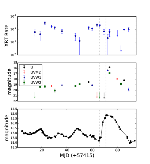
Figure 3: The X-ray, UV and optical light curves of AX J1549.8–5416 are shown in the top, middle and bottom panels, respectively. The rising phase of the outburst is indicated by two vertical dashed lines. The error bars are given at the 1-$\sigma$ level. The observations that only have upper limits are shown by arrows.

3.2 Optical spectra

The average optical spectrum (not corrected for intervening Galactic absorption) of AX J1549.8–5416 (Fig. 4) shows the presence of H_α and H_β Balmer lines, and possibly He I $\lambda$6678, in emission superimposed on an intrinsically blue continuum; the H_β line seems to be embedded in the corresponding absorption feature. All of the detected lines are consistent with being at a redshift of $z$ = 0, indicating that this object is within our Galaxy. Fluxes and equivalent widths (EWs) of the two Balmer lines are: $F_{\rm H_{\alpha}}$ = (8.5$\pm$1.5)$\times$10^-15 erg cm^-2 s^-1; $F_{\rm H_{\beta}}$ = (3$\pm$1)$\times$10^-15 erg cm^-2 s^-1; $EW_{\rm H_{\alpha}}$ = 9.1$\pm$1.6 Å; $EW_{\rm H_{\beta}}$ = 3$\pm$1 Å. No He II emission at 4686 Å is detected down to flux and EW 3-$\sigma$ limits of 2$\times 10^{-15}$ erg cm^-2 s^-1 and 2 Å, respectively. These properties do not vary significantly between the two spectra.

Despite the non-optimal signal-to-noise ratio of the optical spectrum, especially in its blue part, its main characteristics depicted above support the identification of NSV 20407 as a CV. Moreover, the lack of apparent He II emission suggests a non-magnetic nature of the accreting WD in this system (see Warner, 1995, and references therein for details). Also, the observed H_α/H_β flux ratio ($\sim$2.8), when compared with the intrinsic one (2.86; Osterbrock, 1989) is typical of plasmas in accretion in astrophysical conditions, and points to no substantial reddening in the line of sight towards the object.

Figure 4: Averaged spectrum of source NSV 20407 as observed at CASLEO on April 14, 2015 (see text for details). The main spectral features are shown. The symbol $\oplus$ indicates atmospheric telluric absorption bands, while the label ’DIB’ marks the Galactic Diffuse Interstellar Band at 6280 Å.

3.3 X-ray light curve

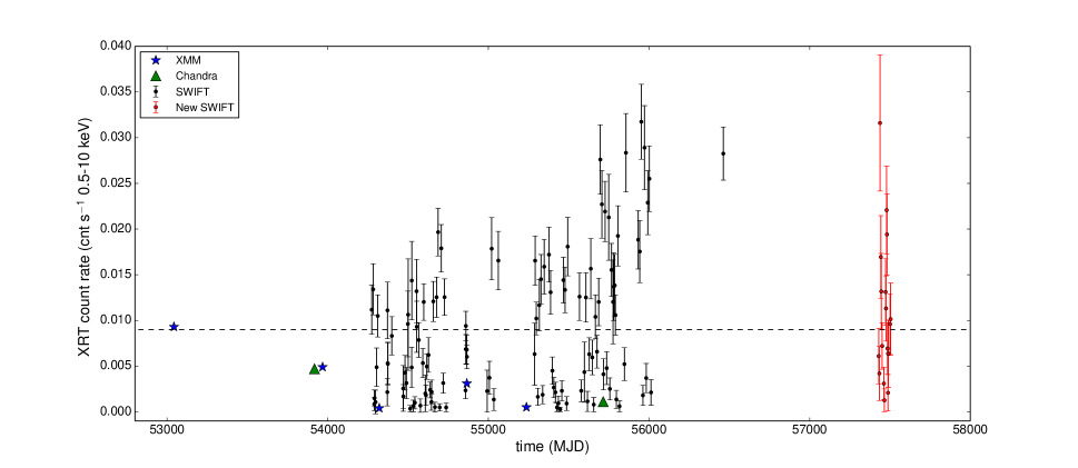
Figure 5: The Swift/XRT light curve of AX J1549.8–5416 (one bin per observation) is represented by black and red (2016 observations) filled circles. The error bars are given at the 1-$\sigma$ level. The blue stars indicate the XMM-Newton EPIC-pn count rate and the green triangles are the Chandra count rate, respectively (converted to the equivalent XRT count rate). The typical spacing between Swift observations is $\sim 1-2$ weeks in the data before 2016. The horizontal dashed line indicates the 0.009 cnt/s level below which the source is in optical outburst.

Fig. 5 shows the long-term X-ray light curve of AX J1549.8–5416 observed by Swift, which indicates its X-ray flux varies by two orders of magnitude. Possibly due to observations being separated by large, irregular amounts of time, we do not find any clear trend in the X-ray light curve.

We converted the XMM-Newton and Chandra count rates to equivalent Swift-XRT count rates using pimms in ftools based on the fitted power law indexes shown in Table 4, with results given in Table 2 and shown in Figure 5, respectively. The longer and more sensitive Chandra and XMM-Newton observations also allowed us to search for significant changes in the X-ray flux on short time-scales. Fig. 6 shows two light curve examples observed by Chandra and XMM-Newton. At a time resolution of 1000 s, the X-ray intensity varied between 0.001 and 0.015 counts/s, and 0.02 and 0.1  counts/s in Chandra and XMM-Newton observations, but no clear outbursts are observed.

We also searched for periodic X-ray variability in these observations, which could correspond to the spin or orbital period of the WD. To search for a periodic modulation in the X-ray light curves we created the Leahy power density spectra (PDS) (Leahy et al., 1983) for each observation. We used the pn and ACIS light curves extracted from the source region and binned at the frame readout time from XMM-Newton and Chandra  respectively. We searched for a periodic behaviour of the source in a range between 73.4 ms and 26.8 hour. No significant periodicity (0.5–10 keV) was found in all XMM-Newton and Chandra observations. We show the 3-$\sigma$ upper limit of the pulsed fraction for each observation in Table 2. The lack of a coherent signal at the WD spin period in the X-ray band suggests that the WD does not possess a strong magnetic field.

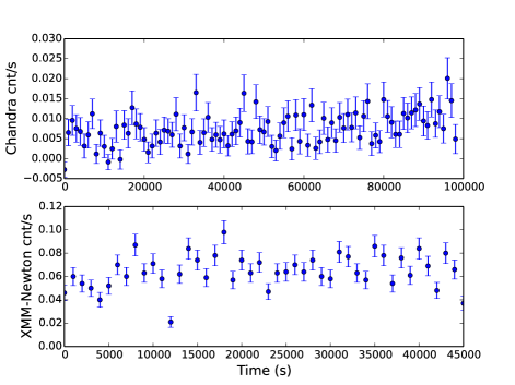
Figure 6: Top panel: the light curve of AX J1549.8–5416 observed by Chandra in Obsid 12554 in Jun 2011; bottom panel: the light curve of the source observed by XMM-Newton in Obsid 0402910101 in Aug 2006. Both light curves are binned at 1000s.

3.4 Multi-wavelength observations in 2016

Fig. 3 shows the X-ray/UV/optical observations of AX J1549.8–5416 from February to May 2016. During the phase when the source showed three mini-outbursts, we do not find a clear trend in the UV bands, probably because of the changes between the UVOT filters. At X-ray energies the source shows $\sim 2$ orders of magnitude variations during these three mini-outbursts. The X-ray flux is highest when the source is in optical quiescence. After the three mini-outbursts, both the optical and UV fluxes decreased and the source went to the quiescent state. The UV emission was not detected before the largest optical outburst.

In the rising phase of the largest optical outburst, the UV emission was still undetected, and the X-ray flux decreased. The UV emission appeared at the time of optical peak, which indicates a UV delay in the rising phase.

Both optical and UV fluxes decreased during the early decaying phase. The X-ray emission was not detectable in this phase. At the end of the outburst the optical and UV fluxes decreased continually, but the X-ray emission recovered. Both the X-ray suppression during the outburst and recovery at the end of the outburst have also been reported in another DN, SS Cyg (Wheatley et al., 2003).

3.5 X-ray $-$ UV and X-ray $-$ optical correlation

Fig. 7 shows the simultaneous UV$-$X-ray intensity correlation diagrams of AX J1549.8–5416 for the four UVOT filters. In the four UV bands, the X-ray flux is to some extend anti-correlated with the UV flux in this source. In order to describe the correlation quantitatively, we used a constant function and a constant plus a power law function to fit the data in four UVOT filters, respectively. The fitting results are shown in Table 3. The f-test probability suggests that, instead of using a constant function, the data can be better fitted by adding a power law function. The power law indices are all negative and indicate that the UV and X-ray are anti-correlated in the four filters. We also performed a Spearman’s rank correlation coefficient test between X-ray and UV fluxes. and report in Table 3 the value of the Spearman’s rank correlation coefficient and the null hypothesis probability (p-value). The negative correlation coefficient and small p-values again indicate that the UV and X-ray are anti-correlated. We note that the observations with upper limits are not used in the above analysis.

Table 3: The fitting parameters of a constant function, a power law with a constant function, correlation coefficient and p-values of Spearman’s rank correlation coefficient test for the UV $-$ X-ray correlation.

data	constant $\chi^{2}$ (dof)	$\Gamma$	power law $+$ constant $\chi^{2}$ (dof)	f-test probably	correlation coefficient	p-value ($\%$)
U	159.7(15)	$-2.2\pm 0.8$	89.5(13)	$2.3\times 10^{-2}$	-0.52	3.87
UVM2	217(14)	$-3.8\pm 1.1$	58.3(12)	$3.7\times 10^{-4}$	-0.54	3.59
UVW1	156(15)	$-0.6\pm 0.2$	29.4(13)	$1.9\times 10^{-5}$	-0.76	0.03
UVW2	120(17)	$-0.2\pm 0.1$	65.5(15)	$3.9\times 10^{-3}$	-0.74	2.03

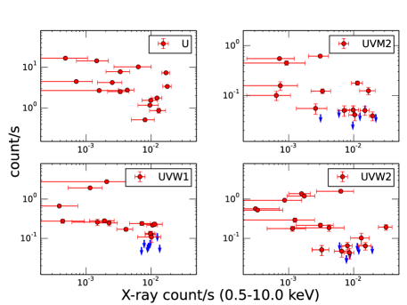
Figure 7: Simultaneous UV$-$X-ray intensity diagrams for four UVOT filters. The error bars are given at the 1-$\sigma$ level. The blue arrows indicate UV upper limits.

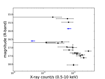
Figure 8: Simultaneous X-ray$-$ optical flux correlation of AX J1549.8–5416. The error bars are given at the 1-$\sigma$ level. The blue arrows indicate X-ray the upper limits.

Fig. 8 shows the simultaneous optical$-$X-ray flux correlation of AX J1549.8–5416 during the 2016 observations. We found that the X-ray and optical flux also show an anti-correlation, which is much clearer at low optical fluxes.

3.6 X-ray Spectral analysis

Due to the low signal-to-noise ratio of this source in an individual Swift XRT observation, spectral fitting is not possible, so we used the X-ray colour to study the X-ray spectra with Swift. For each observation, we calculated the X-ray hardness. We defined the hardness as the count rate in the 2.0–10.0 keV band divided by the count rate in the 0.3–10.0 keV band. In the upper panel of Fig. 9 we show the hardness-intensity diagram (HID) of the source. The data are rebinned so that each bin has approximately the same counts. As shown in the upper panel of Fig. 9, the X-ray spectrum changes with its flux. Above $\sim 2\times 10^{-3}$ cnt/s, the X-ray emission is hard, with a constant hardness ratio $\sim$ 0.6. Below this flux level, its X-ray emission becomes soft. We first fitted these data with a constant function and obtained a $\chi^{2}$ of 151.2 (dof = 17). We then fitted these data with a power-law model, and got a power-law index of $0.57\pm 0.07$ (1-$\sigma$ error) with a $\chi^{2}$ of 41.2 (dof = 16). The smaller reduced $\chi^{2}$ indicates that a power-law fit is better than a constant. We performed a Kolmogorov-Smirnov (K–S) test of our count rates sample against the standard normal distribution. The probability value of K$-$S test is 0.12, which indicates the source count rates are not consistent with random points around a constant value.

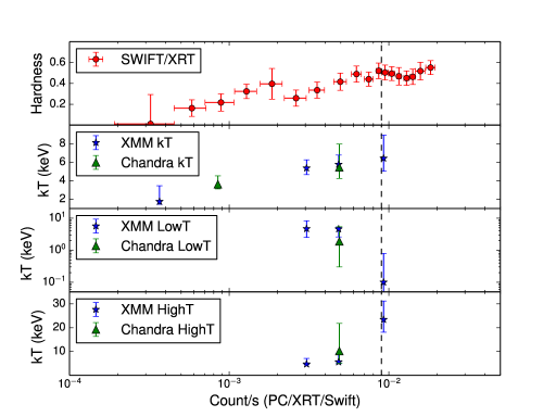
Figure 9: Top panel: the hardness-intensity diagram of AX J1549.8–5416 observed by Swift. Second panel: the plasma temperature (in mekal) as a function of X-ray intensity. Third and fourth panels: the kT_Low and kT_High (in mkcflow) as a function of X-ray intensity. We converted the XMM-Newton and Chandra intensity to equivalent Swift  intensity. The vertical dashed line indicates the 0.009 cnt/s level.

We also measured the X-ray spectrum of the source from four XMM-Newton and two Chandra X-ray observations (observation 0410581901 was not used due to the low count rate and high background). The spectra were fitted in 0.5$-$10 keV range with xspec (v. 12.8.1 Arnaud, 1996). We included the effect of interstellar absorption using wabs assuming cross-sections of Balucinska-Church & McCammon (1992) and solar abundances from Anders & Grevesse (1989), and we let $N_{\rm H}$, the column density along the line of sight, vary during the fitting.

In order to understand the source spectral shape at different flux levels, we first used a power-law model to fit all spectra. The continuum spectra can be well fitted by a power-law model except some residuals around 6.7 keV, which may come from Iron lines. The $N_{\rm H}$ shows comparable values, $\sim(4-5)\times 10^{21}$ cm^-2, in all spectra. The fitted power-law parameters are shown in Table 4. The spectrum photon index is larger when the source is at a low X-ray flux level than at a high X-ray flux level. This is consistent with the XRT X-ray hardness analysis above. There is no need to include a soft component below 1 keV in all spectral fits.

Table 4: Fit statistics and parameters of the spectra models powerlaw and mekal applied to the six X-ray spectrum of AX J1549.8–5416. Error bars are given in 90% confidence levels.

ObsID	$N_{\rm H}$ (PL)	$\Gamma_{\rm PL}$	reduced $\chi^{2}$ (PL)	$N_{\rm H}$ (MK)	kT	norm	reduced $\chi^{2}$ (MK)
	$10^{22}$ cm2			$10^{22}$ cm2	keV	$\times 10^{-4}$
0203910101	$0.38^{+0.11}_{-0.10}$	$1.75^{+0.22}_{-0.21}$	1.01	$0.31^{+0.08}_{-0.07}$	$6.81^{+3.41}_{-1.84}$	$7.4^{+0.5}_{-0.7}$	0.91
7287	$0.36^{+0.27}_{-0.23}$	$1.85^{+0.42}_{-0.38}$	0.94	$0.33^{+0.21}_{-0.18}$	$5.12^{+5.62}_{-1.69}$	$3.4^{+0.7}_{-0.5}$	0.87
0402910101	$0.50^{+0.07}_{-0.06}$	$2.04^{+0.14}_{-0.13}$	1.71	$0.35^{+0.05}_{-0.05}$	$5.45^{+1.00}_{-0.79}$	$3.5^{+0.2}_{-0.2}$	1.21
0560181101	$0.49^{+0.07}_{-0.06}$	$2.05^{+0.16}_{-0.15}$	1.37	$0.36^{+0.05}_{-0.04}$	$5.02^{+0.96}_{-0.75}$	$2.9^{+0.2}_{-0.2}$	1.32
0604880101	$0.52^{+0.33}_{-0.26}$	$3.49^{+1.36}_{-0.91}$	2.21	$0.04^{+0.15}_{-0.04}$	$2.67^{+1.22}_{-0.71}$	$0.35^{+0.10}_{-0.07}$	1.57
12554	$0.45^{+0.34}_{-0.21}$	$2.45^{+0.21}_{-0.19}$	1.21	$0.05^{+0.07}_{-0.04}$	$6.08^{+3.01}_{-1.45}$	$0.77^{+0.07}_{-0.07}$	0.91

As argued above, the optical light curves and spectra indicate the source is a DN. The simple model which is often used in DNe consists of a single-temperature optically thin thermal plasma model (mekal in XSPEC, e.g. Mewe et al., 1985). This model has been successfully used in $\sim$30 spectra of dwarf novae (Baskill et al., 2005) observed with ASCA. We also used this model to fit all our X-ray spectra separately. Because the abundance derived by mekal is consistent with solar abundance within uncertainty, we then fixed the abundance to 1 in our analysis. The fitted parameters are shown in Table 4. With the same degree of freedom and smaller $\chi^{2}$ in each observation, the mekal model gives a better fit than the power-law model.

From Table 4 the $N_{\rm H}$ shows a similar value at different X-ray flux levels. In order to better understand the evolution of the thermal plasma temperature at different flux levels, we fitted the six spectra simultaneously with linked $N_{\rm H}$. The $N_{\rm H}$ value from the simultaneous fitting is ($0.33\pm 0.03$) $\times 10^{22}$ cm², which is comparable with values from individual spectrum fits in Table 5. Fig. 10 shows the X-ray spectrum of each observation (four XMM-Newton and two Chandra) overlaid with best-fitting mekal model. The best-fitting reduced $\chi^{2}$ is 1.29 with 296 degrees of freedom. The iron line is clearly detected in bf the four observations which have higher X-ray flux.

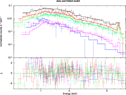
Figure 10: The XMM-Newton PN, and Chandra ACIS spectra of AX J1549.8–5416 in the 0.5$-$10.0 keV energy band. The spectrum was fitted with a single-temperature thin thermal plasma model. The six spectra are represented by six different colour curves in the upper panel. The lower panel shows the residuals to the best-fitting models. The observations 1, 2, 3, 5, 6 and 7 (in Table-2) are shown in black, light blue, red, green, purple and blue, respectively.

Table 5: Fit results for the mekal model applied to six combined X-ray spectra of AX J1549.8–5416. The absorbed 0.5$-$10 keV flux are also reported. Error bars are given at the 90% confidence level. The $N_{\rm H}$ was linked across the spectra and the value is $0.33\pm 0.03\times 10^{22}$ cm².

ObsID	kT	Normalization (MK)	flux (0.5$-$10 keV)
	keV	$10^{-4}$	$10^{-13}$ erg/cm2/s
0203910101	$6.42^{+2.53}_{-1.43}$	$7.56^{+0.56}_{-0.55}$	$11.76^{+1.23}_{-2.05}$
7287	$5.15^{+2.52}_{-1.23}$	$3.47^{+0.35}_{-0.34}$	$5.01^{+0.71}_{-0.51}$
0402910101	$5.76^{+1.03}_{-0.73}$	$3.41^{+0.17}_{-0.16}$	$5.13^{+0.23}_{-0.21}$
0560181101	$5.36^{+0.98}_{-0.78}$	$2.84^{+0.15}_{-0.15}$	$4.15^{+0.19}_{-0.41}$
0604880101	$1.75^{+0.72}_{-0.38}$	$0.43^{+0.13}_{-0.09}$	$0.43^{+0.11}_{-0.12}$
12554	$3.62^{+0.93}_{-0.56}$	$0.96^{+0.07}_{-0.07}$	$1.18^{+0.05}_{-0.09}$

It is clear from Table 5 that the temperature of the thermal plasma is higher when the source has higher X-ray flux. The second panel of Fig.-9 shows the plasma temperature as a function of X-ray intensity. When the source is in the high intensity state, the X-ray spectra show comparable plasma temperature at $\sim 6$ keV. When the source evolves to low intensity levels, the plasma temperature decreases significantly to $\sim$ 1.5 keV. We find that the normalization of mekal also decreases as the X-ray flux decreases.

As discussed in Section 3.5, the large variations in both X-ray and UV bands and the anti-correlation between X-ray and UV emission suggest that the source is a DN (Wheatley et al., 2003; Collins & Wheatley, 2010; Britt et al., 2015). We therefore also used an isobaric cooling flow model, mkcflow, to fit the X-ray emission from the source (Mushotzky & Szymkowiak, 1988). This model is often used to describe the X-ray spectrum of DNe in optical quiescence (Pandel et al., 2005; Mukai et al., 2009; Byckling et al., 2010). Unlike the single temperature plasma model, the cooling flow model is assumed to consist of a range of temperatures. In the model, the temperature varies from the hot shock temperature (kT_High) to the temperature of the optically thin cooling matter (kT_Low) on the WD surface. Thus, cooling flow spectral models should represent a more physically correct picture of the cooling plasma.

Table 6: Fit parameters of the spectral models mkcflow applied to the four X-ray spectra of AX J1549.8–5416. Error bars are given at the 90% confidence level.

ObsID	kTLow	kTHigh	Normalization (MK)	flux (0.5$-$10 keV)
	keV	keV	$10^{-11}\mathrm{M}_{\odot}$ /yr	$10^{-13}$ erg/cm2/s
0203910101	$0.1^{+1.4}_{-0.08}$	$23.5^{+7.8}_{-5.3}$	$10.7^{+3.4}_{-3.3}$	$11.2^{+1.5}_{-3.2}$
7287	$1.9^{+4.8}_{-1.8}$	$10.5^{+20.5}_{-6.1}$	$10.8^{+290.7}_{-7.4}$	$4.8^{+0.2}_{-1.2}$
0402910101	$4.1^{+0.6}_{-2.6}$	$6.3^{+6.2}_{-1.5}$	$65.6^{+223}_{-45.4}$	$4.9^{+0.2}_{-02}$
0560181101	$3.8^{+1.4}_{-2.1}$	$5.8^{+7.6}_{-1.5}$	$120.5^{+354.8}_{-95.4}$	$4.0^{+0.1}_{-0.4}$

Due to the low X-ray count rate and the numerous parameters in mkcflow, we only used this model to fit the spectrum obtained from observations with $>300$ counts. In the following analysis we only used observations 1, 2, 4 and 5 (see Table 2). The parameters are shown in Table 6. We note that, as the X-ray flux decreases, the normalization (accretion rate) increases, kT_Low increases and kT_High decreases. The temperature separation (kT_High – kT_Low ) decreases when the X-ray flux decreases.

Further-more, we first linked the kT_High to the same value in all four observations and then let it be free in observation 1. The $\chi^{2}$ reduced from 278.15 (227 dof) to 268.21 (226 dof). This indicates that the source in observations 2, 4 and 5 has a different X-ray spectrum than that in observation 1.

4 Discussion

4.1 AX J1549.8–5416 is a DN

We have analysed new optical light curves and spectra of the CV AX J1549.8–5416. We detected three outbursts and three mini-outbursts in the 2015 and 2016 optical light curve. We also detected H_α and H_β lines in the optical spectrum. Both the fast rise and exponential decay optical outbursts and the lack of apparent He II emission lines in the optical spectra suggest that AX J1549.8–5416 is a non-magnetic CV. This is not consistent with the MCV classification reported by Lin et al. (2014).

We then analysed all available archival data from Swift, XMM-Newton and Chandra, and find that the source is also highly variable at UV and X-ray wavelengths. We find that the X-ray intensity increases with X-ray hardness. We also find an anti-correlation between X-ray and UV flux in this source. The high-resolution X-ray spectra of XMM-Newton and Chandra can be well described either by a single temperature thermal plasma model or by an isobaric cooling flow model when its X-ray flux is high. The behavior of the X-ray and UV evolution in this system is very similar to other DNe (e.g. SS Cyg, SU UMa, Wheatley et al., 2003; McGowan et al., 2004; Körding et al., 2008), and further confirms that AX J1549.8–5416 is a DN.

From X-ray timing analysis of this system we did not find a significant periodic signal from all XMM-Newton and Chandra observations, which is in common with other DNe. Baskill et al. (2005) analyzed 34 non-MCVs (20 are DNe) observed by ASCA and found that most of the sources do not show periodic modulation of their X-ray flux.

4.2 UV delay and X-ray suppression during the outburst in AX J1549.8–5416

We studied the behaviour of the optical, UV and X-ray emission during the outburst to help us to understand the movement of material through the accretion disc. We observed AX J1549.8–5416 in 2016 with a dedicated optical, UV and X-ray campaign and detected three mini-outbursts and one normal outburst. We find that the UV emission is clearly delayed with respect to the optical emission during the rising phase of the outburst (see Fig. 3). The first optical rise occurred between MJD 57482.04 and 57483.52. The UV emission was still not detectable on MJD 57484.51, so the UV delay must be longer than 1.0 day. The UV became bright on MJD 574487.44, which indicates the UV delay must be less than 5.4 days. Due to the long separation between Swift observations, we can therefore only constrain the delay time to be $\sim 1.0-5.4$ day, The UV delay during the rising phase of DN outbursts has already been reported (e.g., VW Hydri, U Gem and SS Cyg, Cannizzo, 2001; Wheatley et al., 2003). Wheatley et al. (2003) find that in DN SS Cyg the UV emission delays the optical emission by $\sim 1.5-2$ days during the outburst rise, comparable to what we infer for AX J1549.8–5416.

Wheatley et al. (2003) find that in SS Cyg the X-ray flux first rises fast and then drops immediately during the optical outburst rising phase (see also Russell et al., 2016). During the rise of the outburst in AX J1549.8–5416, we also detect X-ray emission significantly lower than that observed before the outburst (quiescence). However, we do not find a spike in X-ray during the outburst rise of AX J1549.8–5416. Since the separation of our Swift observations is $\sim$ 3 days and the duration of the X-ray spike in SS Cyg is $\sim$ 1 day, it is likely that we missed the spike shape variation in our X-ray observations. Similar to SS Cyg we also find the suppression and recovery of the X-ray emission during the middle and the end of the optical outburst, respectively.

Outbursts of DNe are generally interpreted as a sudden brightening of the optically thick accretion disc due to an increased accretion rate (e.g., Osaki, 1996; Lasota, 2001). The UV delay time has been used to measure the heating wave propagation time (Cannizzo, 2001; Wheatley et al., 2003; Schreiber et al., 2003). Unfortunately our optical/UV data are not sufficient to allow us to estimate the beginning and timescale of the propagation of the heating wave.

The suppression of the X-ray emission during an outburst has been interpreted as the boundary layer becoming optically thick to its own radiation. At the end of the outburst the boundary layer switches back to optically thin, the inner disc truncates and emits in the X-ray band (Cannizzo, 2001; Wheatley et al., 2003).

4.3 Mini-outbursts

AX J1549.8–5416 showed three mini-outbursts in the 2016 optical observations. Similar anomalous outbursts have also been observed in SS Cyg (Schreiber et al., 2003). These kind of mini-outbursts cannot be reproduced by the standard disc instability model (DIM). Schreiber et al. (2003) managed to reproduce the mini-outbursts by modifying the DIM. The simulated mini-outburst light curve shows a short rise time and a sharp peak. However, the observed mini-outbursts show rise times ($\sim 9$ days) and similarly slow decays. In their simulations, they assume the disc extends down to the surface of the WD (no truncation) and heating of the outer disc and tidal dissipation are completely neglected.

4.4 X-ray spectra of AX J1549.8–5416 in outburst and quiescence

The X-ray spectra of DNe changes dramatically between optical quiescence and outburst. In quiescence, X-ray spectra are normally described by multi-temperature optically thin thermal models, such as observed from cooling flows. In outburst, the emission is instead described by optically thick emission in the EUV band, with characteristic temperatures around 10 eV. The X-ray spectrum is softer and the temperature is lower than that in optical quiescence (e.g., Baskill et al., 2005; Collins & Wheatley, 2010). In Fig. 9, we show that the plasma temperature decreases as the X-ray flux decreases (optical flux increases). The evolution of X-ray spectra of AX J1549.8–5416 can be well interpreted by the DN hypothesis.

We also used an isobaric cooling flow model to re-analyse the four observations (Obs 1, 2, 3 and 5) when the source had higher X-ray flux. This model is often used to describe the quiescent X-ray spectrum of DNe (Pandel et al., 2005; Mukai et al., 2009; Byckling et al., 2010). The four spectra are well fitted by the cooling flow model. As the X-ray flux decreases, the temperature separation (kT_High – kT_Low) decreases as well, which indicates the X-ray emission became optically thick. This is also consistent with the DN hypothesis (Kuulkers et al., 2006; Patterson, 2011; Balman, 2012).

Ishida et al. (2009) analysed data from Suzaku observations of the DN SS Cyg in quiescence and outburst. They found the maximum temperature of the plasma is $\sim 20$ keV and $\sim 6$ keV in quiescence and outburst, respectively. McGowan et al. (2004) also found that the plasma temperature is $\sim$20 keV when SS Cyg is in quiescence. From Table 6 we find that only Obs 1 has a maximum plasma temperature higher than 20 keV. This suggests that only Obs 1 was observed in quiescence if we assume AX J1549.8–5416 and SS Cyg have comparable maximum plasma temperature in quiescence and outburst. The maximum temperature of the plasma in quiescence is significantly higher than that in outburst in AX J1549.8–5416.

4.5 Duty cycle

In DNe the X-ray flux is always suppressed during optical outbursts and then shows a general anti-correlation with optical flux (Wheatley et al., 2003; McGowan et al., 2004). Since we have a large number of XRT observations, instead of using optical observations, we can use the X-ray data to roughly estimate the duty cycle of AX J1549.8–5416. We define the outburst state when the X-ray intensity is lower than 0.009 cnt/s (see Fig. 5 and 9). This threshold is lower than the equivalent XRT intensity of Obs 1 which was believed to be in quiescence. The calculated duty cycle of AX J1549.8–5416 is $\sim 51\%$. Due to the random and long separation of the XRT observations, the estimated duty cycle may have a large uncertainty. We used highest 10% of the X-ray intensities ($\sim$ 0.003 cnt/s) to estimate the uncertainty of the threshold. With the threshold in the range of 0.006 $-$ 0.012 cnt/s, we estimate a duty cycle in the range of 35% $-$ 60%.

The estimated $\sim$50% duty cycle indicates that this source is a very active DN with comparable quiescence and outburst time. Fig. 3 shows that AX J1549.8–5416 is very active in our new optical observations and also shows comparable quiescence and outburst time. The new optical light curves support the estimated high duty cycle in AX J1549.8–5416.

Britt et al. (2015) recently measured the duty cycles for an existing sample of well-observed, nearby DNe and derived a quantitative empirical relation between the duty cycle of DNe outbursts and the X-ray luminosity of the system in quiescence. If we assume this relationship also applies to AX J1549.8–5416, the estimated $\sim$50% duty cycle suggests the X-ray luminosity of this system should be larger than $10^{32}$ erg/s in quiescence. This suggests that AX J1549.8–5416 might belong to a class of DNe with both high average mass transfer rate in outburst and high instantaneous accretion rate in quiescence. Assuming the X-ray flux of this source in quiescence is larger than $\sim$1.2$\times 10^{-13}$ erg/cm²/s (see Table 5), we could estimate the distance to AX J1549.8–5416 to be $\mathrel{\mathchoice{\lower 0.5pt\vbox{\halign{$\mathnew\displaystyle\hfil#\hfil$\cr<\crcr\sim\crcr}}}{\lower 0.5pt\vbox{\halign{$\mathnew\textstyle\hfil#\hfil$\cr<\crcr\sim\crcr}}}{\lower 0.5pt\vbox{\halign{$\mathnew\scriptstyle\hfil#\hfil$\cr<\crcr\sim\crcr}}}{\lower 0.5pt\vbox{\halign{$\mathnew\scriptscriptstyle\hfil#\hfil$\cr<\crcr\sim\crcr}}}}$ 1.0 kpc. We note that neither the duty cycle nor the X-ray luminosity in quiescence are able to entirely reliably trace the mass accretion rate of the system (Britt et al., 2015).

5 Conclusions

In this paper we analyse new optical/UV/X-ray light curves and spectra of the peculiar CV AX J1549.8–5416. Both the FRED optical outbursts and the lack of apparent He II emission lines in the optical spectra suggest that AX J1549.8–5416 is a typical DN. We present multi-wavelength (optical/UV/X-ray) observations of DN AX J1549.8–5416 throughout three mini-outbursts and one normal outburst. We find the UV emission delays the optical emission by $1.0-5.4$ days during the rising phase of the outburst. The X-ray emission shows suppression during the outburst peak and recovery during the end of the outburst.

We also analyse archival Swift, Chandra and XMM-Newton observations of AX J1549.8–5416. We find an approximately anti-correlation between X-ray and UV flux. The high-resolution X-ray spectra from XMM-Newton and Chandra can be well described either by a single temperature thermal plasma model or by an isobaric cooling flow model when its X-ray flux is high. We find the maximum temperature of the plasma in quiescence is significant higher than that in outburst in AX J1549.8–5416. Our estimated high duty cycle suggests that the X-ray luminosity of this source should be larger than $10^{32}$ erg/s in quiescence.

Appendix A Log of LCOGT 2015 and 2016 observations.

We observed the field of AX J1549.8–5416 with LCOGT suite of robotic 1-m telescopes in 2015 and 2016. Some data in 2016 were taken with the 2-m Faulkes Telescope South (FTS). All 1-m telescopes are equipped with a camera with pixel scale 0.467 arcsec pixel^-1; this is 0.304 arcsec pixel^-1 for the 2-m data. We adopt a 2.8 arcsec aperture for the 1-m data and 1.8 arcsec aperture for the 2-m data, to match the average seeing differences between the 1-m and 2-m data. The observation logs are provided in Table 7 and the telescopes are:

1m0-03 $=$ Siding Spring, Australia
1m0-05 $=$ Cerro Tololo, Chile
1m0-10 $=$ SAAO, South Africa
1m0-11 $=$ Siding Spring, Australia
1m0-12 $=$ SAAO, South Africa
1m0-13 $=$ SAAO, South Africa
FTS $=$ 2m telescope at Siding Spring, Australia

Table 7: Log of LCOGT 2015 and 2016 observations.

Date UT	MJD	magnitude ($R$)	Telescope	Filters	Exposure times (s)
2015-04-30	57142.81028	$17.471\pm 0.051$	1m0-10	$B,V,R,i^{\prime}$	100,100,100,100
2015-05-06	57148.06933	$15.589\pm 0.014$	1m0-05	$B,V,R,i^{\prime}$	200,100,100,100
2015-05-12	57154.42698	$16.530\pm 0.016$	1m0-11	$B,V,R,i^{\prime}$	200,100,100,100
2015-05-25	57167.10270	$17.051\pm 0.034$	1m0-10	$B,V,R,i^{\prime}$	200,100,100,100
2015-06-06	57179.70814	$17.684\pm 0.062$	1m0-12	$R$	100
2015-06-07	57180.72358	$17.285\pm 0.033$	1m0-13	$R$	100
2015-06-10	57183.00197	$15.604\pm 0.046$	1m0-10	$R$	100
2015-06-10	57183.00341	$15.552\pm 0.059$	1m0-10	$R$	100
2015-06-10	57183.00483	$15.535\pm 0.047$	1m0-10	$R$	100
2015-06-10	57183.00637	$15.623\pm 0.036$	1m0-10	$R$	100
2015-06-10	57183.00809	$15.609\pm 0.038$	1m0-10	$R$	100
2015-06-10	57183.00970	$15.592\pm 0.043$	1m0-10	$R$	100
2015-06-10	57183.01119	$15.582\pm 0.036$	1m0-10	$R$	100
2015-06-10	57183.01262	$15.598\pm 0.051$	1m0-10	$R$	100
2015-06-10	57183.01405	$15.528\pm 0.073$	1m0-10	$R$	100
2015-06-10	57183.36087	$15.512\pm 0.012$	1m0-03	$R$	100
2015-06-10	57183.36218	$15.513\pm 0.012$	1m0-03	$R$	100
2015-06-10	57183.36349	$15.499\pm 0.013$	1m0-03	$R$	100
2015-06-10	57183.36481	$15.509\pm 0.012$	1m0-03	$R$	100
2015-06-10	57183.36612	$15.509\pm 0.012$	1m0-03	$R$	100
2015-06-10	57183.36744	$15.502\pm 0.013$	1m0-03	$R$	100
2015-06-10	57183.36875	$15.514\pm 0.011$	1m0-03	$R$	100
2015-06-10	57183.37007	$15.489\pm 0.011$	1m0-03	$R$	100
2015-06-10	57183.37138	$15.501\pm 0.010$	1m0-03	$R$	100
2015-06-10	57183.37270	$15.509\pm 0.010$	1m0-03	$R$	100
2015-06-10	57183.99798	$15.527\pm 0.010$	1m0-05	$R$	100
2016-02-01	57419.66520	$16.796\pm 0.040$	1m0-03	$R$	200
2016-02-01	57419.69488	$16.764\pm 0.017$	1m0-03	$R$	200
2016-02-03	57421.08700	$17.022\pm 0.092$	1m0-10	$R$	200
2016-02-04	57422.29909	$16.981\pm 0.017$	1m0-05	$R$	200
2016-02-05	57423.33328	$17.041\pm 0.025$	1m0-05	$R$	200
2016-02-06	57424.03382	$17.124\pm 0.022$	1m0-13	$R$	200
2016-02-07	57425.03107	$17.118\pm 0.022$	1m0-13	$R$	200
2016-02-07	57425.72135	$17.146\pm 0.024$	FTS	$R$	120
2016-02-08	57426.02834	$16.963\pm 0.019$	1m0-10	$R$	200
2016-02-09	57427.02551	$17.095\pm 0.038$	1m0-13	$R$	200
2016-02-09	57427.68389	$17.026\pm 0.033$	FTS	$R$	120
2016-02-10	57428.02394	$17.026\pm 0.021$	1m0-13	$R$	200
2016-02-10	57428.63314	$16.994\pm 0.020$	FTS	$R$	120
2016-02-11	57429.04155	$16.992\pm 0.019$	1m0-13	$R$	200
2016-02-12	57430.02881	$16.947\pm 0.019$	1m0-10	$R$	200
2016-02-12	57430.62836	$16.880\pm 0.019$	FTS	$R$	120
2016-02-13	57431.11716	$16.795\pm 0.034$	1m0-13	$R$	200
2016-02-14	57432.01188	$16.757\pm 0.017$	1m0-13	$R$	200
2016-02-14	57432.69475	$16.691\pm 0.016$	FTS	$R$	120
2016-02-15	57433.26795	$16.607\pm 0.013$	1m0-05	$R$	200
2016-02-15	57433.62776	$16.642\pm 0.023$	FTS	$R$	120
2016-02-16	57434.26027	$16.590\pm 0.013$	1m0-05	$R$	200
2016-02-16	57434.68099	$16.562\pm 0.022$	FTS	$R$	120
2016-02-17	57435.27446	$16.713\pm 0.014$	1m0-05	$R$	200
2016-02-17	57435.67131	$16.947\pm 0.079$	FTS	$R$	120
2016-02-18	57436.01093	$16.803\pm 0.016$	1m0-10	$R$	200
2016-02-18	57436.34304	$16.918\pm 0.015$	1m0-05	$R$	200
2016-02-18	57436.61226	$17.040\pm 0.025$	FTS	$R$	120
2016-02-19	57437.25208	$17.138\pm 0.024$	1m0-05	$R$	200
2016-02-19	57437.65759	$17.195\pm 0.026$	FTS	$R$	120
2016-02-20	57438.25358	$17.264\pm 0.030$	1m0-05	$R$	200
2016-02-21	57439.29170	$17.274\pm 0.032$	1m0-05	$R$	200
2016-02-22	57440.00040	$17.559\pm 0.069$	1m0-13	$R$	200
2016-02-23	57441.01024	$17.417\pm 0.046$	1m0-13	$R$	200
2016-02-24	57442.00571	$17.492\pm 0.047$	1m0-13	$R$	200
2016-02-25	57443.02726	$17.485\pm 0.044$	1m0-13	$R$	200

-1

Table 7: Continued.

Date UT	MJD	magnitude ($R$)	Telescope	Filters	Exposure times (s)
2016-02-27	57445.62117	$17.318\pm 0.053$	1m0-03	$R$	200
2016-02-28	57446.01335	$17.420\pm 0.035$	1m0-13	$R$	200
2016-03-01	57448.06750	$17.008\pm 0.018$	1m0-10	$R$	200
2016-03-01	57448.62489	$17.028\pm 0.021$	1m0-03	$R$	200
2016-03-03	57450.60801	$17.112\pm 0.018$	1m0-03	$R$	200
2016-03-04	57451.60506	$17.130\pm 0.018$	1m0-03	$R$	200
2016-03-05	57452.60201	$17.313\pm 0.021$	1m0-03	$R$	200
2016-03-07	57454.40306	$17.337\pm 0.024$	1m0-05	$R$	200
2016-03-07	57454.62370	$17.337\pm 0.022$	1m0-03	$R$	200
2016-03-09	57456.36274	$17.483\pm 0.023$	1m0-05	$R$	200
2016-03-09	57456.94641	$17.457\pm 0.024$	1m0-13	$R$	200
2016-03-10	57457.58832	$17.391\pm 0.025$	1m0-03	$R$	200
2016-03-11	57458.58716	$17.275\pm 0.020$	1m0-03	$R$	200
2016-03-12	57459.63460	$17.106\pm 0.019$	1m0-03	$R$	200
2016-03-13	57460.74649	$16.931\pm 0.020$	1m0-03	$R$	200
2016-03-14	57461.63193	$16.717\pm 0.014$	1m0-03	$R$	200
2016-03-15	57462.96572	$16.552\pm 0.025$	1m0-13	$R$	200
2016-03-16	57463.93002	$16.539\pm 0.015$	1m0-13	$R$	200
2016-03-17	57464.56933	$16.648\pm 0.017$	1m0-03	$R$	200
2016-03-18	57465.61511	$16.686\pm 0.026$	1m0-03	$R$	200
2016-03-20	57467.91649	$17.066\pm 0.033$	1m0-13	$R$	200
2016-03-21	57468.00108	$17.096\pm 0.025$	1m0-10	$R$	200
2016-03-22	57469.16480	$17.188\pm 0.039$	1m0-05	$R$	200
2016-03-23	57470.15458	$17.210\pm 0.031$	1m0-13	$R$	200
2016-03-24	57471.14439	$17.373\pm 0.049$	1m0-13	$R$	200
2016-03-26	57473.64500	$17.209\pm 0.035$	1m0-03	$R$	200
2016-03-27	57474.74986	$17.387\pm 0.035$	1m0-03	$R$	200
2016-03-28	57475.26752	$17.307\pm 0.033$	1m0-05	$R$	200
2016-03-29	57476.02154	$17.393\pm 0.057$	1m0-13	$R$	200
2016-03-29	57476.37488	$17.288\pm 0.036$	1m0-05	$R$	200
2016-03-30	57477.36813	$17.600\pm 0.040$	1m0-05	$R$	200
2016-04-02	57480.52608	$17.793\pm 0.033$	1m0-03	$R$	200
2016-04-03	57481.13232	$17.424\pm 0.026$	1m0-05	$R$	200
2016-04-03	57481.13548	$17.550\pm 0.030$	1m0-05	$R$	200
2016-04-04	57482.04207	$17.424\pm 0.045$	1m0-13	$R$	200
2016-04-05	57483.51738	$15.862\pm 0.009$	1m0-03	$R$	200
2016-04-07	57485.12103	$15.458\pm 0.007$	1m0-05	$R$	200
2016-04-07	57485.12456	$15.460\pm 0.007$	1m0-05	$R$	200
2016-04-07	57485.14465	$15.440\pm 0.007$	1m0-05	$R$	200
2016-04-07	57485.16703	$15.451\pm 0.007$	1m0-05	$R$	200
2016-04-07	57485.17373	$15.451\pm 0.008$	1m0-05	$R$	200
2016-04-07	57485.34353	$15.399\pm 0.007$	1m0-05	$R$	200
2016-04-07	57485.41653	$15.415\pm 0.007$	1m0-05	$R$	200
2016-04-07	57485.51197	$15.424\pm 0.011$	1m0-03	$R$	200
2016-04-07	57485.51545	$15.426\pm 0.013$	1m0-03	$R$	200
2016-04-08	57486.13174	$15.170\pm 0.007$	1m0-05	$R$	200
2016-04-08	57486.19285	$15.132\pm 0.006$	1m0-05	$R$	200
2016-04-08	57486.86447	$15.173\pm 0.007$	1m0-13	$R$	200
2016-04-09	57487.17049	$15.152\pm 0.006$	1m0-05	$R$	200
2016-04-11	57489.93411	$15.247\pm 0.007$	1m0-10	$R$	200
2016-04-12	57490.49836	$15.307\pm 0.008$	1m0-03	$R$	200
2016-04-13	57491.17433	$15.313\pm 0.006$	1m0-05	$R$	200
2016-04-15	57493.49691	$15.665\pm 0.012$	1m0-03	$R$	200
2016-04-16	57494.16704	$15.848\pm 0.010$	1m0-13	$R$	200
2016-04-18	57496.48241	$16.362\pm 0.017$	1m0-03	$R$	200
2016-04-19	57497.30683	$16.587\pm 0.018$	1m0-05	$R$	200
2016-04-24	57502.85855	$17.373\pm 0.035$	1m0-10	$R$	200
2016-04-24	57502.88819	$17.508\pm 0.046$	1m0-13	$R$	200
2016-04-26	57504.85539	$18.029\pm 0.052$	1m0-10	$R$	200
2016-04-27	57505.50374	$17.827\pm 0.065$	1m0-03	$R$	200
2016-04-27	57505.87528	$17.951\pm 0.046$	1m0-13	$R$	200
2016-04-30	57508.80454	$17.788\pm 0.037$	1m0-13	$R$	200

References

- Anders & Grevesse (1989) Anders E., Grevesse N., 1989, Geochim. Cosmochim. Acta, 53, 197
- Arnaud (1996) Arnaud K. A., 1996, in G. H. Jacoby & J. Barnes ed., Astronomical Data Analysis Software and Systems V Vol. 101 of Astronomical Society of the Pacific Conference Series, XSPEC: The First Ten Years. p. 17
- Balman (2012) Balman S., 2012, MnSAI, 83, 585
- Balucinska-Church & McCammon (1992) Balucinska-Church M., McCammon D., 1992, ApJ, 400, 699
- Baskill et al. (2005) Baskill D. S., Wheatley P. J., Osborne J. P., 2005, MNRAS, 357, 626
- Blackburn (1995) Blackburn J. K., 1995, in Shaw R. A., Payne H. E., Hayes J. J. E., eds, Astronomical Data Analysis Software and Systems IV Vol. 77 of Astronomical Society of the Pacific Conference Series, FTOOLS: A FITS Data Processing and Analysis Software Package. p. 367
- Britt et al. (2015) Britt C. T., Maccarone T., Pretorius M. L., Hynes R. I., Jonker P. G., Torres M. A. P., Knigge C., Johnson C. O., Heinke C. B., Steeghs D., Greiss S., Nelemans G., 2015, MNRAS, 448, 3455
- Brown et al. (2009) Brown P. J., Holland S. T., Immler S., Milne P., Roming P. W. A., Gehrels N., Nousek J., Panagia N., Still M., Vanden Berk D., 2009, AJ, 137, 4517
- Burrows et al. (2005) Burrows D. N., Hill J. E., Nousek J. A., Kennea J. A., Wells A., Osborne J. P., Abbey A. F., Beardmore A., Mukerjee K., Short A. D. T., Chincarini G., Campana S., Citterio O., Moretti A., Pagani C., 2005, Space Sci. Rev., 120, 165
- Byckling et al. (2010) Byckling K., Mukai K., Thorstensen J. R., Osborne J. P., 2010, MNRAS, 408, 2298
- Cannizzo (2001) Cannizzo J. K., 2001, ApJ, 556, 847
- Chen et al. (1997) Chen W., Shrader C. R., Livio M., 1997, ApJ, 491, 312
- Collins & Wheatley (2010) Collins D. J., Wheatley P. J., 2010, MNRAS, 402, 1816
- Evans et al. (2009) Evans P. A., Beardmore A. P., Page K. L., Osborne J. P., O’Brien P. T., Willingale R., Starling R. L. C., Burrows D. N., Godet O., Vetere L., Racusin J., Goad M. R., Wiersema K. a., 2009, MNRAS, 397, 1177
- Ezuka & Ishida (1999) Ezuka H., Ishida M., 1999, ApJS, 120, 277
- Fruscione et al. (2006) Fruscione A., McDowell J. C., Allen G. E., Brickhouse N. S., Burke D. J., Davis J. E., Durham N., 2006, 6270, 1
- Gandhi et al. (2010) Gandhi P., Dhillon V. S., Durant M., Fabian A. C., Kubota A., Makishima K., Malzac J., Marsh T. R., Miller J. M., Shahbaz T., Spruit H. C., Casella P., 2010, MNRAS, 407, 2166
- Henden et al. (2015) Henden A. A., Levine S., Terrell D., Welch D. L., 2015, in American Astronomical Society Meeting Abstracts Vol. 225 of American Astronomical Society Meeting Abstracts, APASS - The Latest Data Release. p. 336.16
- Horne (1986) Horne K., 1986, PASP, 98, 609
- Ishida et al. (2009) Ishida M., Okada S., Hayashi T., Nakamura R., Terada Y., Mukai K., Hamaguchi K., 2009, PASJ, 61, S77
- Jordi et al. (2006) Jordi K., Grebel E. K., Ammon K., 2006, A&A, 460, 339
- Körding et al. (2008) Körding E., Rupen M., Knigge C., Fender R., Dhawan V., Templeton M., Muxlow T., 2008, Science, 320, 1318
- Kuulkers et al. (2006) Kuulkers E., Norton A., Schwope A., Warner B., 2006, X-rays from cataclysmic variables. pp 421–460
- Lasota (2001) Lasota J., 2001, New Astronomy Review, 45, 449
- Leahy et al. (1983) Leahy D. A., Darbro W., Elsner R. F., Weisskopf M. C., Kahn S., Sutherland P. G., Grindlay J. E., 1983, ApJ, 266, 160
- Lewis et al. (2008) Lewis F., Russell D. M., Fender R. P., Roche P., Clark J. S., 2008, in Proc. VII Microquasar Workshop: Microquasars and Beyond, Proceedings of Science. SISSA, Trieste, PoS(MQW7)069
- Lin et al. (2014) Lin D., Webb N. A., Barret D., 2014, ApJ, 780, 39
- Maitra & Bailyn (2008) Maitra D., Bailyn C. D., 2008, ApJ, 688, 537
- McGowan et al. (2004) McGowan K. E., Priedhorsky W. C., Trudolyubov S. P., 2004, ApJ, 601, 1100
- Mewe et al. (1985) Mewe R., Gronenschild E. H. B. M., van den Oord G. H. J., 1985, A&AS, 62, 197
- Meyer & Meyer-Hofmeister (1981) Meyer F., Meyer-Hofmeister E., 1981, A&A, 104, L10
- Mukai et al. (2009) Mukai K., Zietsman E., Still M., 2009, ApJ, 707, 652
- Mushotzky & Szymkowiak (1988) Mushotzky R. F., Szymkowiak A. E., 1988, in Fabian A. C., ed., NATO Advanced Science Institutes (ASI) Series C Vol. 229 of NATO Advanced Science Institutes (ASI) Series C, Einstein Observatory solid state detector observations of cooling flows in clusters of galaxies. pp 53–62
- Osaki (1996) Osaki Y., 1996, PASP, 108, 39
- Osterbrock (1989) Osterbrock D. E., 1989, Astrophysics of gaseous nebulae and active galactic nuclei
- Pandel et al. (2003) Pandel D., Córdova F. A., Howell S. B., 2003, MNRAS, 346, 1231
- Pandel et al. (2005) Pandel D., Córdova F. A., Mason K. O., Priedhorsky W. C., 2005, ApJ, 626, 396
- Patterson (2011) Patterson J., 2011, MNRAS, 411, 2695
- Russell et al. (2011) Russell D. M., Maitra D., Dunn R. J. H., Fender R. P., 2011, MNRAS, 416, 2311
- Russell et al. (2016) Russell T. D., Miller-Jones J. C. A., Sivakoff G. R., Altamirano D., O’Brien T. J., Page K. L., Templeton M. R., Koerding E. G., Knigge C., Rupen M. P., Fender R. P., Heinz S., Maitra D., 2016, MNRAS, 460, 3720
- Saitou et al. (2012) Saitou K., Tsujimoto M., Ebisawa K., Ishida M., 2012, PASJ, 64, 88
- Samus et al. (2009) Samus N. N., Durlevich O. V., et al. 2009, VizieR Online Data Catalog, 1, 2025
- Schreiber et al. (2003) Schreiber M. R., Hameury J.-M., Lasota J.-P., 2003, A&A, 410, 239
- Singh (2013) Singh K. P., 2013, in Das S., Nandi A., Chattopadhyay I., eds, Astronomical Society of India Conference Series Vol. 8 of Astronomical Society of India Conference Series, X-ray emission from magnetic cataclysmic variables. pp 115–122
- Sugizaki et al. (2001) Sugizaki M., Mitsuda K., Kaneda H., Matsuzaki K., Yamauchi S., Koyama K., 2001, ApJS, 134, 77
- Tody (1993) Tody D., 1993, in Hanisch R. J., Brissenden R. J. V., Barnes J., eds, Astronomical Data Analysis Software and Systems II Vol. 52 of Astronomical Society of the Pacific Conference Series, IRAF in the Nineties. p. 173
- Van de Sande et al. (2015) Van de Sande M., Scaringi S., Knigge C., 2015, MNRAS, 448, 2430
- Warner (1995) Warner B., 1995, Cambridge Astrophysics Series, 28
- Wheatley et al. (2003) Wheatley P. J., Mauche C. W., Mattei J. A., 2003, MNRAS, 345, 49