On a new theoretical framework for RR Lyrae stars II: Mid–Infrared Period–Luminosity–Metallicity Relations

Abstract

We present new theoretical period-luminosity-metallicity (PLZ) relations for RR Lyræ stars (RRL) at Spitzer and WISE wavelengths. The PLZ relations were derived using nonlinear, time-dependent convective hydrodynamical models for a broad range in metal abundances (Z=0.0001 to 0.0198). In deriving the light curves, we tested two sets of atmospheric models (Brott & Hauschildt, 2005; Castelli & Kurucz, 2003) and found no significant difference between the resulting mean magnitudes. We also compare our theoretical relations to empirical relations derived from RRL in both the field and in the globular cluster M4. Our theoretical PLZ relations were combined with multi-wavelength observations to simultaneously fit the distance modulus, $\mu_{0}$, and extinction, $A_{V}$, of both the individual Galactic RRL and of the cluster M4. The results for the Galactic RRL are consistent with trigonometric parallax measurements from Gaia’s first data release. For M4, we find a distance modulus of $\mu_{0}=11.257\pm 0.035$ mag with $A_{V}=1.45\pm 0.12$ mag, which is consistent with measurements from other distance indicators. This analysis has shown that when considering a sample covering a range of iron abundances, the metallicity spread introduces a dispersion in the PL relation on the order of 0.13 mag. However, if this metallicity component is accounted for in a PLZ relation, the dispersion is reduced to $\sim 0.02$ mag at MIR wavelengths.

1 Introduction

RR Lyræ (RRL) variables are a popular tracer for old stellar populations, thanks to their abundance in the globular clusters, halos and bulges of galaxies (see e.g. Vivas & Zinn 2006; Dékány et al. 2013; Pietrukowicz et al. 2015). During their advanced evolutionary phases low and intermediate-mass stars cross the so-called Cepheid instability strip (a region of the HR diagram in which stellar atmospheres are pulsationally stable). Unlike their higher mass counterparts, RRLs do not appear to obey well defined period-luminosity (PL) relations at visible wavelengths. As a consequence, their usefulness as distance indicators has been historically limited to the adoption of a luminosity-metallicity relation characterized by a rather large ($\approx 5$%) intrinsic scatter (Cáceres & Catelan, 2008). This relation also suffers from evolutionary effects and uncertainties related to the metallicity scale and/or $\alpha$ enhancement. Moreover, the relation is possibly nonlinear across the whole observed RRL metallicity range (Caputo et al., 2000).

Several theoretical and empirical arguments, however, indicate that RRLs become solid distance indicators when moving from the optical to the infrared bands. As described as length in Bono et al. (2016b), the main reasons are three-fold:

1. As first demonstrated over 30 years ago by Longmore et al. (1986) and again by Dall’Ora et al. (2004), an obvious PL relation does appear moving from the optical to the infrared bands. While the slope is vanishingly small in the $V$-band, it becomes steeper with increasing wavelength (Catelan et al., 2004; Marconi et al., 2015), ranging from $-1.2$ in the $R$-band to $-2.2$ in the $K$-band. This behavior is different than the one shown by Cepheids (Bono et al., 1999) and is related to the specific dependence of the RRL bolometric correction with temperature (Bono et al., 2001, 2003; Bono, 2003). For $\lambda\gtrsim 2.2\ \mu$m the slope of the PL relations of instability strip pulsators (both Cepheids and RRLs) becomes almost constant. In this wavelength regime the brightness variations of pulsating stars is mainly driven by their radius variation, and the effective temperature variations only play a minimal role (Jameson, 1986; Madore & Freedman, 2012).

2. The intrinsic dispersion of the RRL PL relations steadily decreases when moving from the optical to the infrared bands. This trend is due to the fact that starting from the near-infrared (NIR) cooler RRLs are steadily brighter than hotter ones, due to the stronger temperature sensitivity of the bolometric correction (Bono, 2003). As a consequence, infrared PL relations are only marginally affected by the intrinsic width in temperature of the instability strip, since they almost mimic a period-luminosity-color relation. Furthermore, the instability strip itself becomes narrower at longer wavelengths, and as a consequence the color term responsible for the intrinsic dispersion on the PL relations vanishes (Catelan et al., 2004; Madore & Freedman, 2012; Marconi et al., 2015). This means that at MIR wavelengths PL relations provide for more precise distance indicators (Braga et al., 2015).

3. Infrared observations are less affected by reddening, due to the power-law dependency of the extinction laws ($\lambda^{-\beta}$, with $\beta\sim 1.6$ to $1.8$; Bono et al. 2016b). This translates into a smaller uncertainty of reddening and differential reddening, when compared to the $V$-band, by a factor ranging from four ($J$) to ten ($K$). In the $L$ and $M$ bands extinction is further reduced, reaching its minimum values with $A_{V}/A_{\lambda}\approx 15$ and 20, respectively. This is a huge advantage when inspecting highly- and differentially-reddened targets, such as those in the Galactic bulge (Nishiyama et al., 2009).

To explore the detailed physics behind these remarkable properties, Marconi et al. (2015) used new, time- and metal-dependent convective hydrodynamic models to derive a theoretical calibration for the period-luminosity-metallicity (PLZ), period-Wesenheit-metallicity (PWZ) and metal-independent period-Wesenheit (PW) relations of RRL. These relations have been published in the optical (Johnson-Kron-Cousins’s $BVRI$) and NIR (2MASS $JHK$) wavelength regimes (Marconi et al., 2015), and tested by fitting average magnitudes of RRLs in the M4 (NGC 6121) Galactic globular cluster (Braga et al., 2015) and in the dwarf spheroidal galaxy Carina (Coppola et al., 2015). On the other hand, similar analysis in the mid-infrared (MIR), where the extinction is lower and the intrinsic temperature-dependent scatter is at its smallest, is lagging. Several authors (Klein et al., 2011; Madore et al., 2013; Neeley et al., 2015) have derived empirical calibrations for Galactic RRL MIR PL relations, but their zero point calibration is based on just five stars for which $\approx 10$% accuracy Hubble Space Telescope (HST) Fine Guidance Sensor (FGS) parallaxes are available (Benedict et al., 2011). A detailed theoretical analysis of RRL PLZ relations in the MIR is missing. To fill this gap we decided to extend the detailed investigation of RRL pulsation properties provided by Marconi et al. (2015) in order to derive a theoretical calibration of RRL PLZ and PWZ relations in the MIR. In this paper we focus on the MIR bands available to the InfraRed Array Camera (IRAC, Fazio et al. 2004) onboard the Spitzer Space Telescope (Werner et al., 2004), as well as the passbands of the Wide-field Infrared Survey Explorer (WISE, Wright et al. 2010).

Our choice of filters is motivated by two reasons. Firstly, both IRAC and WISE provide a large archive of Galactic and extragalactic observations with thousands of RRL observed in one or multiple epochs. These include the “warm” Spitzer observational campaigns part of the Carnegie RR Lyrae Program (CRRP; Freedman et al., 2012) and the Spitzer Merger History and Shape of the Halo program (SMHASH; Johnston et al., 2013), designed to obtain multi-epoch light-curves of RRLs in the halo and bulge of the Milky Way, as well as in dwarf galaxies and tidal streams. Secondly, the wavelength range covered by IRAC and WISE will be available as part of the James Webb Space Telescope (JWST) Near Infrared Camera (NIRCam) and the Mid-Infrared Instrument (MIRI) imagers. The NIRCam wide filters F356W and F444W, in particular, are analogous to the IRAC warm passbands at 3.6 and 4.5 $\micron$. The predicted sensitivity of these two filters (13.8 and 24.5 nJy for F356W and F444W for a 10$\sigma$ detection in 10,000 sec integration) will allow the detection of RRLs at a distance modulus as high as $\sim 26$ mag (1.6 Mpc), thereby covering a significant portion of the Local Group, at least in galaxies where the $\sim 0.2$ arcsec resolution will be sufficient to beat confusion. This will open the possibility of using RRL distances to precisely calibrate secondary distance indicators independently from Cepheids, with the goal to provide a Population II route to the cosmological distance scale (Beaton et al., 2016).

A detailed description of the models, and the procedure we followed to derive the PLZ and PWZ relations in the IRAC and WISE bands, is presented in Section 2. To test the reliability of our theoretical relations in providing accurate distance estimates of individual stars, we have collected average magnitudes for a sample of Galactic RRLs with a broad range of metallicity, as well as revised our previously published photometry for the RRLs in the globular cluster M4. These observations are presented in Section 3. We compare our theoretical PLZ relations to empirical PL and PLZ relations from the literature in Section 4. In Sections 5 and 6 we use our synthetic PLZ relations to fit new distance moduli and visual band extinctions for Galactic and M4 RRL, respectively, and compare these results to other estimates. The conclusions of our work, with a focus on the dependence of the PLZ relations on metallicity, are presented in Section 7.

2 Theoretical framework

Theoretical models allow us to derive new theoretical MIR PLZ relations, by adopting the same models and following the same steps described in Marconi et al. (2015). For a detailed discussion on the models, see Section 2 of the quoted paper. Here, we want to stress only a few major points.

1. The models span a large range in metallicity. Seven different values of $Z$ ranging from 0.0001 to 0.0198 ($\alpha$-enhanced chemical mixture) are taken into account.

2. For each metallicity, either two or three luminosity levels are included for fundamental (FU) or first overtone (FO) pulsators, to take into account evolved RRLs that are brighter than the ZAHB. The three possible luminosity levels are $\log{L_{ZAHB}}$ (A), $\log{L_{ZAHB}}$ + 0.1 (B), and $\log{L_{ZAHB}}$ + 0.2 with mass 10% lower than the other models (C).

3. The effective temperatures range between 7200 (bluest model on the ZAHB) to 5300 K (reddest model of the brightest luminosity level) with steps of 100 K. The individual A, B, and C sequences include from four to eleven FU models and from two to seven FO models. This range covers the temperature width of the instability strip.

In Marconi et al. (2015) we transformed the bolometric light curves of the quoted grid into the 2MASS JHK and the UBVRI photometric bands using the bolometric corrections and color-temperature relations obtained from the synthetic spectra provided by Castelli & Kurucz (2003). To transform the same models into the IRAC and the WISE photometric bands, we decided to perform a test to estimate the impact that different sets of synthetic spectra have on MIR bands. In particular, we used the atmosphere models provided by Brott & Hauschildt (2005) (covering $2700~{}\mathrm{K}<T_{eff}<10,000$ K and $-0.5\leq\log g\leq 0.5$) and by Castelli & Kurucz (2003) (covering $3500~{}\mathrm{K}<T_{eff}<50,000$ K and $0.0\leq\log g\leq 5.0$). The adopted synthetic spectra are available for a wide range of [Fe/H], namely for $-4.0<$ [Fe/H] $<+0.5$. The Brott & Hauschildt (2005) spectra are also available for several [$\alpha$/Fe] values in [-0.2, +0.8] with a spacing of 0.2 dex, while the Castelli & Kurucz (2003) ones are computed only for [$\alpha$/Fe]=0.0 and +0.4. For present calculations we adopted the spectra with [$\alpha$/Fe]=$+0.4$ in both cases. Since the two spectral libraries adopt different assumptions concerning the solar abundances (the Brott & Hauschildt (2005) adopted the Grevesse & Noels (1993) solar abundances whereas the Castelli & Kurucz (2003) the ones from Grevesse & Sauval (1998)), we placed them on the same scale by converting the [Fe/H] of each synthetic spectrum into the total metallicity $Z$. The relation used for this conversion is $\log(Z/X)-\log(Z/X)\sun=[Fe/H]+0.35$ where $\log(Z/X)\sun=-1.61$ (Pietrinferni et al., 2006).

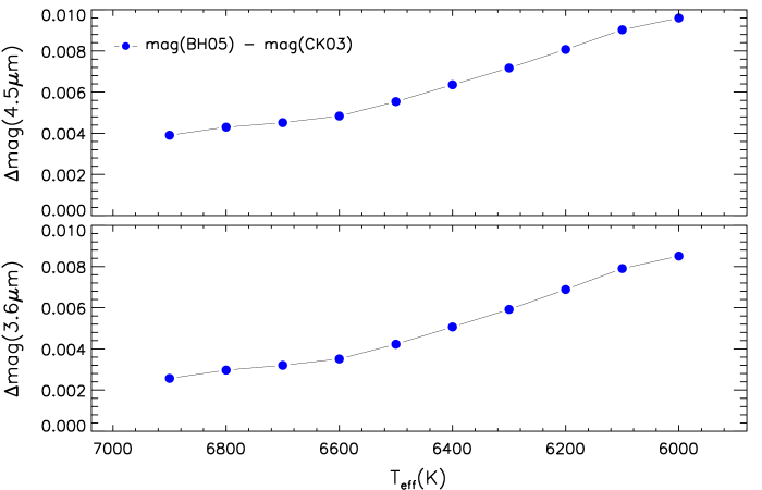
Figure 1: Top: Difference in [4.5] magnitudes as a function of the effective temperature for a set of FU models computed at fixed stellar mass (0.716 $M_{\odot}$), luminosity ($\log L/L_{\odot}=1.72$), and chemical composition ($Z=0.0003,Y=0.245$). Bolometric light curves predicted by hydrodynamical pulsation models were transformed into the observational plane by using color-temperature relations provided by Castelli & Kurucz (2003) and by Brott & Hauschildt (2005). $T_{eff}$ spans the range between the blue and red edge of the instability strip. Bottom: Same as the top, but for the [3.6] magnitudes.

We obtained the bolometric corrections (BC) for all the $T_{\mathrm{eff}}$, $\log\,g$ and [Fe/H] ($Z$) values available in the spectral library. Then, we computed the magnitudes by interpolating the BC tables at the requested $T_{\mathrm{eff}}$, $\log\,g$ and total metallicity $Z$ along each bolometric light curve. The transformations were computed for the two different sets of atmosphere models and we found that the difference is negligible. Data plotted in Figure 1 display that the difference in MIR mean magnitudes ranges from a few thousandths close to the blue (hot) edge of the instability strip to at most one hundredth of a magnitude close to the red (cool) edge of the instability strip. Data plotted in this figure refer to a sequence of FU models constructed at fixed mass, luminosity, and chemical composition (see labeled values). However, the difference is minimal over the entire grid of models. For the above reasons and for homogeneity with previous predictions, we decided to use the BC and the CT relations provided by Castelli & Kurucz (2003).

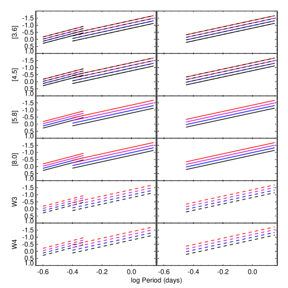
Figure 2: Predicted RRL period-luminosity-metallicty relations for IRAC (solid lines) and WISE (dashed lines) bands. Left panels show separate RRc and RRab relations, while the right panels show the fundamentalized relations. Four metallicities are plotted: [Fe/H] $=0$ (bottom black line), [Fe/H]$=-1.0$ (blue line), [Fe/H]$=-2.0$ (purple line), and [Fe/H] $=-3.0$ (top red line).

Finally, we have fitted the periods, mean magnitudes and metallicities—now transformed into iron abundances—and obtained the coefficients of the PLZ relations. The mean magnitudes for the entire grid of models are given in Tables 1 and 2 for the FO and FU pulsators respectively. The coefficients are given in Table 3, and the relations for four metallicities ([Fe/H] from 0 to -3.0 dex) are plotted in Figure 2. Preliminary results based on two different metal abundances and three different helium contents indicate that pulsation properties of RR Lyrae are minimally affected by the helium content. The key variation between models with canonical and enhanced helium content is the luminosity, and in turn the pulsation period (Marconi et al., 2011). A more detailed investigation will be addressed in a forthcoming paper (Marconi et al. 2017, in preparation), where the entire grid of model light curves, from the optical to MIR bands and covering the entire range in metallicity and helium abundance of RRL, will also be published.

We also obtained the coefficients for two and three band period-Wesenheit-metallicity (PWZ) relations, where the Wesenheit magnitude is defined as $W(B_{1},B_{2})=M_{B_{1}}-\alpha(M_{B_{1}}-M_{B_{2}})$ or $W(B_{1},B_{2},B_{3})=M_{B_{1}}-\alpha(M_{B_{2}}-M_{B_{3}})$. The coefficients of the color term, $\alpha$, have been fixed according to the reddening law we have adopted (Cardelli et al., 1989). The coefficients for the color term and the PWZ relations are given in Tables 4 and 5 for two and three bands PWZ. For readers interested in the coefficients of the PWZ relation assuming a different reddening law, we provide a Python program, in which you can input the coefficients ($A_{\lambda}/A_{V}$) of an alternative reddening law, and it will output the corresponding coefficients of the PWZ relation. The full versions of Tables 1, 2, 4, and 5 are available in the online journal and portions are shown here for form and content.

By comparing the results described above with those obtained by Marconi et al. (2015) in their Table 6, we outline that i) The dispersion of the relations is constant (within 0.01 mag) in the wavelength range from the $H$ to the $W4$ band, with values of the order of $\sigma_{FO}$=0.02 mag, $\sigma_{FU}$=0.03-0.04 mag and $\sigma_{FO+FU}$=0.04 mag. ii) The metallicity coefficient shows no significant wavelength dependence from the $R$ to the IRAC bands, and is mainly due to the change in luminosity. This is because the metallicity dependence of the BCs effectively cancels out the change in $T_{\mathrm{eff}}$, resulting in a minimal change in color ($\sim 0.01$ mag or less over the entire [Fe/H] range) as you increase metallicity.

3 Optical, NIR, and MIR data

To test the model PLZ relations described in Section 2, we have compiled multi-wavelength observations for a sample of 55 nearby Galactic RRL. The sample was based on stars included in the Hipparcos catalog, limited to stars with $V<11$ mag, $A_{V}<0.5$, and an expected final Gaia parallax with 2-3% accuracy. Most of the observations were collected as part of the Carnegie RR Lyrae Program (CRRP, PID 90002), and were published in Monson et al. (2017). The pulsation period, metallicity, extinction, and available distance moduli of the stars in our sample are listed in Table 6. In addition to the Galactic sample, we compiled observations of RRL in the globular cluster M4. All data has been homogenized to the following photometric system: Kron-Cousins RI, 2MASS $JHK_{s}$, Spitzer S19.2 3.6 and 4.5 $\micron$, Spitzer S18.25 5.8 and 8.0 $\micron$, and WISE $W1$, $W2$ and $W3$ (see Monson et al., 2017, for details).

3.1 Galactic RRL

The $RIJHK$ data set was built from three sources: Monson et al. (2017), Klein (2014), and Feast et al. (2008). The data set from Monson et al. (2017) combines observations collected for CRRP with the Three-Hundred Millimeter telescope with archival observations from individual studies (and places them on a homogeneous photometric system), and was used as the basis for our sample of Galactic RRL. For stars without multi-epoch observations in this data set, we supplemented with the multi-epoch observations available in Klein (2014). Light curves from Klein (2014) were obtained with the Nickel 1 meter telescope at Lick Observatory and 1.3 meter PAIRITEL telescope at the Fred Lawrence Whipple Observatory and were fit with Fourier series. Finally, Feast et al. (2008) presented a procedure to estimate mean magnitudes from single epoch 2MASS JHK measurements of RRL. For any stars still missing multi-epoch $JHK$ observations from the previous two data sets, we adopted the estimated mean magnitude from Feast et al. (2008). The Feast et al. (2008) templates are not very precise, and we derived a single uncertainty for each band according to the standard deviation of the residuals between the template mean magnitude and derived mean magnitude of stars for which we have well sampled light curves. This results in uncertainties in the adopted mean magnitudes of 0.06, 0.04, and 0.07 mag for $JHK$, respectively.

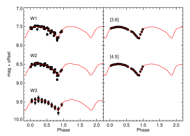
Figure 3: Sample WISE and IRAC light curves for the Galactic RRL star, SU Dra. The W1, [3.6] and W3 bands are offset by $\pm 1$ mag for better visibility. The smoothed light curve generated by GLOESS is shown as the red line.

Mid-infrared observations for our sample are also presented in Monson et al. (2017), that combined the Spitzer 3.6 and 4.5 $\micron$ observations obtained for CRRP with WISE photometry. The first two bands in the WISE photometric system are very similar to the IRAC bands, but we have elected to keep the WISE and IRAC photometry separate in this paper for two main reasons. First, for most of the stars in our sample, adding in WISE photometry degrades the quality of our IRAC light curves (Figure 3 compares the quality of WISE and IRAC light curves side by side). Second, the WISE and IRAC passbands are not identical, and it is unclear if there is an offset between the two calibrations. When comparing the average magnitudes of RRL obtained with Spitzer and WISE, Monson et al. (2017) saw a small offset. However, the AllWISE explanatory supplement  found no offset with the first two IRAC bands. Given this unresolved discrepance, we re-derived the average magnitudes separately for the IRAC and WISE data presented in Monson et al. (2017). The IRAC light curves are covered by a minimum of 24 epochs over a single pulsation cycle (some stars were observed with up to 134 epochs to fill gaps in Spitzer’s schedule). We note that the Spitzer Science Center (SSC) recently released the final calibration of warm mission Spitzer data (S19.2). The new calibration included new flux conversions, linearity solution for the 3.6 $\micron$ band, and flat fields, and is now consistent with the final cryogenic mission calibration (S18.25) defined by Carey et al. (2012). The WISE photometry comes from the AllWISE data release, and provides an average of 36, 36, and 18 random epochs in the $W1$, $W2$, and $W3$ bands, respectively.

The GLOESS method (Neeley et al., 2015; Monson et al., 2017, and references therein) was used to fit smoothed light curves and derive the mean intensity magnitude in each of the bands. For stars in common with the CRRP sample, we found no significant difference in the mean magnitudes fit with fourier series (Klein, 2014) and the GLOESS method (Monson et al., 2017). The final count for each band is as follows: 32 in R, 55 in I, 54 in J, 53 in H, 54 in K, 51 in [3.6], 51 in [4.5], 55 in W1, 55 in W2, and 54 in W3.

3.2 M$4$ RRL

Photometry for the RRL in the globular cluster M4 is presented in Stetson et al. (2014) ($RIJHK$) and in Neeley et al. (2015) (Spitzer [3.6] and [4.5]). The $RIJHK$ data were assembled from $\sim 65$ data sets mostly taken at the VLT. The IRAC 3.6 and 4.5 $\micron$ photometry presented in Neeley et al. (2015) was collected as part of CRRP, and has been updated in this paper to the most recent Spitzer calibration (S19.2) using the same calibration procedure as for the Galactic RRL. All photometry was undertaken using the DAOPHOT/ALLSTAR/ALLFRAME (Stetson, 1987, 1992, 1994) suite of programs.

For this work, we have also performed new photometry of single-epoch archival observations of M4 from Spitzer’s cryogenic mission 5.8 and 8.0 $\micron$ bands. The cluster was observed with a medium scale 11-point cycling dither pattern, with a frame time of 100 seconds. Aperture photometry was performed on Basic Calibrated Data (BCDs) generated by the S18.25 pipeline with a 3-3-7 pixel aperture, and calibrated to the photometric system defined by Carey et al. (2012). The aperture corrections used were 1.1356 and 1.2255 at 5.8 and 8.0 $\micron$ respectively. Photometry at the 11 dither positions was averaged to obtain a single measurement. These observations were obtained 8 years before the CRRP Spitzer observations, and we were unable to reliably determine the pulsation phase and construct a template to estimate the mean magnitude. Therefore we elected to use the single epoch observation as the estimated mean magnitude with an uncertainty equal to half the amplitude in the 3.6 or 4.5 $\micron$ bands. These results as well as the updated mean magnitudes from Neeley et al. (2015) are available in Table 7.

4 Empirical PL relations

We can directly compare our synthetic PLZ relations with some recent empirical relations. Since many empirical measurements have been made on single metallicity populations (i.e. in globular clusters), the metallicity component has not been reliably measured and only PL relations are available. One exception to this is the empirical PLZ relation in the $W1$ and $W2$ bands measured using several globular clusters (Dambis et al., 2014). Both the period slope and the zero point are consistent between the theoretical and empirical methods. However the metallicity term they measure (0.096 mag/dex in $W1$ and 0.108 mag/dex in $W2$) is smaller than in our synthetic PLZ relations by about $4\sigma$, but we note that their method is reliant on the accuracy of the visual band magnitude - metallicity relation. Madore et al. (2013) also measured PL relations in the WISE bands, but using only four RRab stars with parallax measurements. Due to their limited sample, the uncertainties on their derived parameters are very large ($\pm 0.9$ mag in slope, $\pm 0.2$ mag in the zero point), and they were not able to see a metallicity dependence (these four stars also cover an extremely limited range in [Fe/H]).

We have recently completed a multi-wavelength analysis of the PL relation for the globular cluster M4 (NGC 6121). The $RIJHK$ relations were presented in Braga et al. (2015) and IRAC 3.6 and 4.5 $\micron$ relations were originally presented in Neeley et al. (2015). For consistency, we have updated the calibrated relations from Neeley et al. (2015) to the new Spitzer S19.2 calibration, as well as extended the relations to the 5.8 and 8.0 $\micron$ bands. The new first overtone, fundamental, and fundamentalized relations are given in Table 8. For the 3.6 and 4.5 $\micron$ bands, the slope was fixed using the cluster RRL, and the zero point was determined using five Galactic RRL (RR Lyr, RZ Cep, SU Dra, UV Oct, and XZ Cyg) with geometric parallaxes measured using the $HST$ Fine Guidance Sensor (Benedict et al., 2011). The $\sigma$ quoted is the dispersion of the cluster RRL around the PL relation. The fundamentalized calibrated relations result in a distance modulus of $\mu_{0}=11.353\pm 0.095$ at 3.6 $\micron$ and $\mu_{0}=11.363\pm 0.095$ at 4.5 $\micron$, assuming extinction values calculated specifically for M4 ($A_{V}=1.39\pm 0.01$ and $R_{V}=3.62$) in Hendricks et al. (2012). For the longer 5.8 and 8.0 $\micron$ bands, the slope is based on single epoch photometry of the M4 RRL, so the uncertainties and dispersion are significantly larger. In addition, no photometry of the five calibrating RRL was available in these bands, so the calibrated zero point is determined by applying the average distance modulus measured from the 3.6 and 4.5 $\micron$ bands to the apparent zero point.

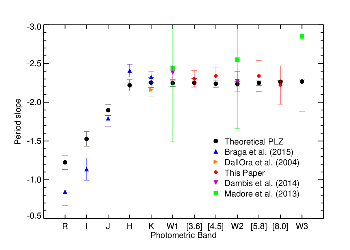
Figure 4: The period dependence ($b_{\lambda}$) for different filters. The predicted coefficients of PLZ relations from Marconi et al. (2015) and Table 3 of this work are shown as black circles. Empirical measurements from the literature are shown for comparison according to the legend.

A comparison between the period dependence derived from theoretical methods and the empirical methods described above is shown in Figure 4. The theoretical period dependence is shown as filled circles, and empirically derived slopes are over-plotted according to the legend. Overall the predicted period dependence in all bands is consistent with results from the literature, and we do observe the predicted flattening of the period dependence at longer wavelengths. The observed slope of the PL relation in M4 is within $1\sigma$ of the predicted slope in the $J$, $K$, and IRAC bands. In the $R$, $I$ and $H$ bands, the slope of the observed PL relations differs from the predicted relation by 2, 2.7, and 2$\sigma$ respectively. This discrepancy could be due to the larger scatter in the PL relation at shorter wavelengths, but we note that we find a better agreement with the synthetic HB - based slopes by Catelan et al. (2004) in these bands. Ongoing work on more globular clusters in the CRRP sample will help to better characterize the period dependence in the RRL PLZ relation.

5 Galactic RRL distances

In addition to simply comparing theoretical and empirical results, we can use our synthetic PLZ relations to fit the data and obtain predicted distance moduli and extinctions for all of the RRL in our sample. We used the synthetic PLZ relations to obtain predicted absolute magnitudes, $M_{\lambda}$, in the $RIJHK$, IRAC, and WISE bands. From these predicted absolute magnitudes, reddened distance moduli ($m_{\lambda}-M_{\lambda}$) were calculated, and then used in combination with a universal reddening law to fit both the true distance modulus ($\mu_{0}$) and visual band extinction ($A_{V}$) of each star using a weighted least squares fit of the form

$$m_{\lambda}-M_{\lambda}=\mu_{0}+A_{V}(A_{\lambda}/A_{V})$$ (1)

where $A_{\lambda}/A_{V}$ are the coefficients of the reddening law. This technique was first introduced by Freedman et al. (1985, 1991) and has recently been employed on Classical Cepheids by Gieren et al. (2005) and Inno et al. (2016). The reddening law we adopted was that of Cardelli et al. (1989), which we extended into the IRAC and WISE bands according to Indebetouw et al. (2005) and Madore et al. (2013) respectively. The weights in the fit were determined by the sum in quadrature of the uncertainties in the apparent mean magnitudes and predicted absolute magnitudes of the star, where the uncertainty of the predicted absolute magnitude is given by the dispersion of the PLZ relation of the corresponding wavelength. As a consequence, the IRAC bands have the most weight in determining the distance modulus, since the PLZ relations have the lowest dispersion at these wavelengths, and the IRAC mean magnitudes are more precise than those determined with WISE data. The shorter wavelengths provide the leverage necessary to fit the extinction. The results of this fit are given in the last two columns of Table 6.

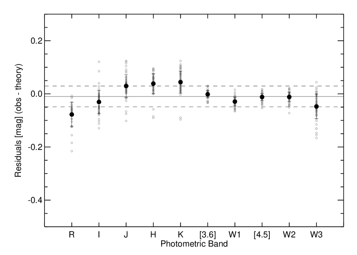
Figure 5: Residual between the absolute magnitude using the best fit distance moduli and extinctions and the predicted absolute magnitude from theoretical PLZ relations for all galactic RRL in each band. Individual stars are shown with open circles, and the average residual for each band is shown as a filled circle. The error bars represent the standard deviation in the residuals of the individual stars. The solid line is the weighted mean of the average residuals, and the dashed lines are $1\sigma$ from the mean. Note that because this is a weighted fit, the solid line passes the points with the most weight ([3.6] and [4.5]) and not through zero.

To assess the ability of the theoretical PLZ relation to fit the distance moduli of all sample stars at different wavelengths, we have transformed all average magnitudes into semi-empirical absolute magnitudes using the best fit distance moduli and extinctions from Table 6. The residuals between the calculated (from observed apparent magnitude) and predicted (from the PLZ relation) absolute magnitudes in each band are shown in Figure 5. Individual stars are shown as small open circles, while the average residual in each band is over-plotted as filled circles. The dashed lines represent the standard deviation around the mean of the average residuals. The IRAC, W1, and W2 bands offer the smallest dispersion. Predicted absolute magnitudes in the $JHK$ bands tend to be brighter than the calculated absolute magnitude. There are three possibilities for this discrepancy: 1) the reddening law is inappropriate for these bands, 2) mean magnitudes calculated from $JHK$ templates are systematically too faint, or 3) the color temperature relations used to transform the bolometric light curves into the observational plane are incorrect for NIR wavelengths. The first point is unlikely, because the effect of reddening is low at NIR wavelengths, and the coefficients of the reddening law would have to change by as much as 50%. We see no systematic offset between mean magnitudes derived from $JHK$ templates and observed light curves, but we note that less than half the stars in our sample have NIR light curves with high enough phase coverage to measure an accurate mean magnitude. Further observations are needed to see if this resolved the discrepancy with theory, or if the color temperature relations need some adjustment in the $JHK$ bands.

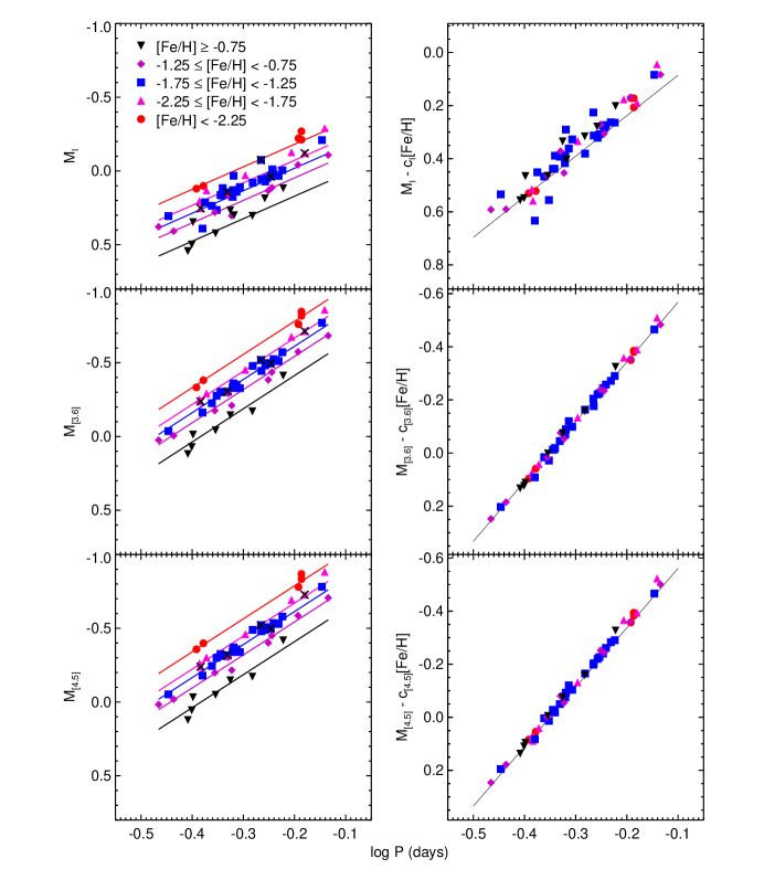
Figure 6: Calculated absolute magnitude versus period of field RRL stars for the I, 3.6, and 4.5 $\micron$ bands. Left panels – The stars have been separated into metallicity bins from low (black triangles) to high (red circles) metal abundance. Predicted relations for the median of each metallicity bin are shown with solid lines. Right panels – The metallicity term ($c_{\lambda}*[Fe/H]$) has been subtracted from the vertical axis (normalized to solar metallicity, [Fe/H]=0.0 dex.

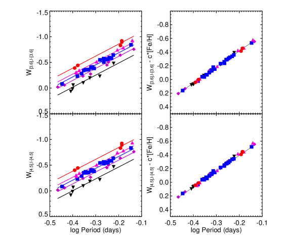
Figure 7: Period-Wesenheit-metallicity relation of field RRL stars. Predicted relations for the five metallicity bins are shown with solid lines. In the right panel the metallicity term has been subtracted form the vertical axis.

In Klein (2014), a multi-wavelength approach similar to ours was used to fit distances and extinctions of RRL, but the effects of metallicity were ignored. In their Figure 6.20, PL relations from optical to MIR are shown with remarkably small scatter. However the scatter is by design artificially small, since the optimal solution is estimated minimizing the residuals of the different bands. Our synthetic PLZ relations provide a method to estimate the effect of metallicity on the determination of distances. The left panels of Figure 6 show how the RRL in our sample lie in the period-magnitude plane when metallicity is ignored. Stars were divided into five metallicity bins, and the predicted PL relation for the median of each bin is shown as the solid line in the corresponding color. The dispersion around individual relations is quite low (with much of it still due to a spread in metallicity), but if you consider all RRL covering a large range of metallicity as a single population, the dispersion around the average metallicity is large (0.12, 0.13, and 0.13 in the $I$, [3.6], and [4.5] bands respectively). In the right panels of Figure 6, the metallicity term has been subtracted out, and the vertical axis is now $M_{\lambda}-c_{\lambda}[Fe/H]$. Now the dispersion around the theoretical relation is almost an order of magnitude smaller (0.053, 0.019, and 0.017 mag in the $I$, [3.6], and [4.5] bands respectively). These panels illustrate the drastic improvement you can expect in the accuracy of distance determinations when accounting for metallicity. Assuming the theoretical PLZ relations correctly characterize the effect on the zero point due to metallicity, using PLZ relations over PL relations will reduce the uncertainty of distance measurements from 13% to 2%. A similar argument can be shown using PWZ relations (Figure 7). Here, the dispersion in the PW relation once metallicity has been removed is even smaller (0.012 mag for $I$-IRAC PWZ relations). This could be because PWZ relations are reddening free (they depend only on the reddening law, not the extinction of individual objects), or because the PWZ relations include a color term and reduce the scatter because they take into account the width in temperature of the instability strip.

5.1 Comparison with HST

Prior to the Gaia release, the only geometric measurement of RRL distances was the parallax of five stars (RR Lyr, RZ Cep, SU Dra, UV Oct, and XZ Cyg) measured using HST Fine Guidance Sensor (Benedict et al., 2011). With only five calibrators available, the precision of the absolute zero point of RRL PL relations has been severely limited. In this section, we compare the HST parallaxes with results based on the theoretical PLZ relations.

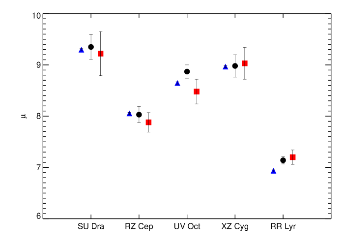
Figure 8: A direct comparison of the distance modulus of five stars obtained with three methods: 1) the method presented in this paper (blue triangles), 2) HST parallax measurements from Benedict et al. (2011) (black circles), and 3) proper motion parallaxes from TGAS (red squares). For both the HST and TGAS distance moduli, the error bars are dominated by the error in the parallax.

Table 6 presents the distance moduli and extinction derived in Benedict et al. (2011), compared with the value estimated in this work. The distance moduli comparison is also shown in Figure 8. Two stars, RR Lyr and UV Oct, exhibit a 2.7 and 1.6$\sigma$ tension, respectively, between our method and the HST distance moduli. Three stars (RR Lyr, SU Dra, and UV Oct) are also fit with a significantly larger extinction using our method. The extinctions adopted in Benedict et al. (2011) are from Feast et al. (2008), where stars were fit using 3-D Galactic extinction models while assuming a distance based on $M_{V}-[Fe/H]$ or preliminary $PL(K)$ relations. Figure 9 compares the residuals with predicted absolute magnitude when correcting observations using the HST parallaxes and extinctions (left panel) as a function of wavelength. The residuals of four stars (RR Lyr, RZ Cep, SU Dra, and UV Oct) present a trend with wavelength when using the HST derived parameters, indicating the extinction assumed for these stars in Benedict et al. (2011) is incorrect. The vertical offset seen in RR Lyr and UV Oct is a consequence of the difference in distance modulus we measure. In contrast, the right panel shows no offsets or trends, suggesting good agreement with theory across all wavelengths. Clearly, the observations and theory are at odds for some of these stars. The discrepancy with predicted absolute magnitude shows no trend with period, distance, or metallicity, which indicates the problem may lie with individual parallax and extinction measurements. We should note that both RR Lyr and UV Oct exhibit the Blazhko effect, and it is possible that this is affecting the mean magnitude of these stars. However, XZ Cyg is also a Blazhko star, and all methods are in good agreement for this star.

5.2 Comparison with Gaia DR1

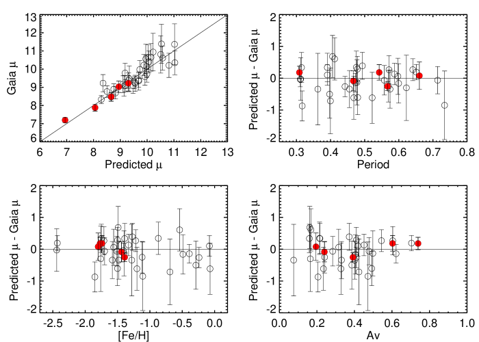
Figure 10: Top left: One-to-one comparison of the distance moduli derived in this paper and determined from the first release of TGAS parallaxes. The five stars with previously determined HST parallaxes are highlighted with closed red circles. Given that all but two stars agree within $1\sigma$, this may indicate that the TGAS errors are overestimated as suggested in Casertano et al. (2016) and Gould et al. (2016). Top right: Residuals between predicted and TGAS parallaxes as a function of the pulsation period. Bottom left: Residuals between predicted and TGAS parallaxes as a function of the metal abundance. Bottom right: Residuals between predicted and TGAS parallaxes as a function of the fitted visual band extinction.

We can also compare the distance moduli obtained above with the recent parallax measurements from the Gaia mission. Gaia’s first data release (DR1) became public on September 14, 2016 (Gaia Collaboration et al., 2016a, b). This release included proper motion parallax measurements for stars in common with the Tycho-2 catalog, and are based on the Tycho-Gaia astrometric solution (TGAS, Michalik et al., 2015). TGAS parallaxes were available for 41 of the stars in our sample, with uncertainties ranging from $\sigma_{\pi}/\pi=0.06$ to $\sigma_{\pi}/\pi=0.83$. The distance moduli from TGAS parallaxes are given in Table 6. In Figure 10 we compare the TGAS results with the distance moduli obtained in this paper for stars with $<55\%$ uncertainty in the TGAS parallax. The top right panel is a one to one comparison between the two methods. The five stars with previously determined HST parallaxes are highlighted with filled red circles. For the majority of stars, the methods agree within $1\sigma$. Only four stars (AM Tuc, RR Lyr, MT Tel, V Ind) are outliers, and all are within 2$\sigma$. Both the dispersion and individual uncertainty increases with distance. The dispersion is 0.30 for stars with $\mu_{0}<9.5$ and 0.46 for stars with $\mu_{0}>9.5$, and the average uncertainty in the TGAS distance is twice as large for stars with $\mu_{0}>9.5$ mag. The remaining panels in Figure 10 show the residual between the two methods as a function of stellar parameters, indicating there are no trends with period, metallicity, or $A_{V}$. This confirms that the residual error between our best fit value and the TGAS parallax are likely due to the statistical uncertainties in the TGAS results.

6 M4 distance

We can use globular clusters as an additional laboratory to test the theoretical PLZ relations. Globular clusters offer the advantage that there are many RRL at roughly the same distance, reddening, and metallicity. For the closest globular cluster to us, M4 (NGC 6121), if we assume a 10pc radius the expected difference in distance modulus between stars in the front and back of the cluster is about 0.02 mag. Since this is smaller than the expected dispersion in the PLZ relation, we cannot accurately measure the distances and extinctions for individual stars. However, we can measure the average distance and extinction for the cluster as a whole.

The distance modulus and reddening to M4 was fit in a similar method to the Galactic RRL, but instead of fitting an individual distance and extinction for each star, we derived the average $\mu_{0}$ and $A_{V}$. A reddened distance modulus for each band was calculated by averaging the difference between observations and predicted absolute magnitude from the theoretical PLZ relations. The true distance modulus and visual extinction were then fit using a least squares fit as in Equation 1, but now the reddening coefficients $A_{\lambda}/A_{V}$ are defined by a reddening law specific to M4 (Hendricks et al., 2012). This reddening law accounts for the fact that the cluster is behind the $\rho$ Oph cloud by adopting a higher dust parameter ($R_{V}=3.62$) than the Cardelli law ($R_{V}=3.1$). Figure 11 shows the extinction corrected distance moduli for each band. Single epoch archival data for the two longer Spitzer bands are also shown for reference as open circles, but were not included in the fit. The dashed lines represent how the uncertainty in extinction propagates with wavelength. The final distance modulus is $\mu_{0}=11.257\pm 0.035$, and the $V$ band extinction is $A_{V}=1.45\pm 0.12$. This is consistent with our results from purely empirical NIR and MIR PL relations, $\mu_{0}=11.283\pm 0.010\pm 0.018$ (Braga et al., 2015), $\mu_{0}=11.353\pm 0.095$ at 3.6 $\micron$ and $\mu_{0}=11.363\pm 0.095$ at 4.5 $\micron$ (Section 4) respectively. Our measured distance modulus of $\mu_{0}=11.257$ is also consistent with recent measurements from a variety of other primary distance methods, and we will highlight a few here (see Section 2 of Braga et al., 2015, for a more complete discussion). Hendricks et al. (2012) estimates $A_{V}=1.39\pm 0.01$ and $\mu_{0}=11.28\pm 0.06$ so our measurements are within $1\sigma$. The distance to M4 has also recently been measured by Kaluzny et al. (2013) using three eclipsing binary stars. They obtained $\mu_{0}=11.30\pm 0.05$, which is also in agreement with our method.

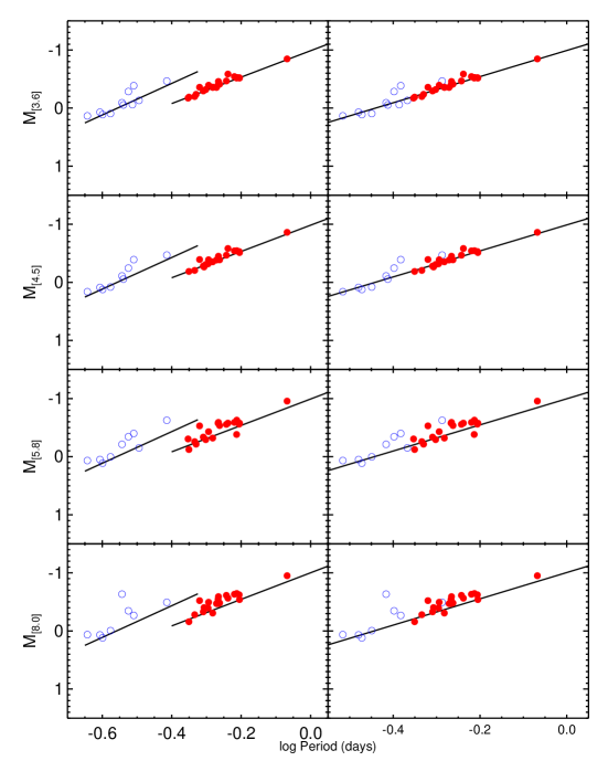
Figure 12: MIR photometry of M4 RRL corrected to absolute magnitude using best fit distance and extinction. RRc stars are shown with open blue circles and RRab stars with filled red circles. The theoretical PL relations for the cluster’s metallicity is shown as the black lines. As in Figure 2, the left panels show separate relations for the RRc and RRab stars and in the right panels the RRc stars have been fundamentalized.

Figure 12 shows the MIR observations transformed into absolute magnitude with the best fit distance modulus and extinction. Fundamental pulsators (RRab) are shown with filled red circles while first overtone pulsators (RRc) are shown as open blue circles. In the right panels, the period of the RRc variables have been fundamentalized. The theoretical PL relation for the metallicity of the cluster ([Fe/H]=-1.1) is over-plotted. The bottom two panels show the first PL relations at the 5.8 and 8.0 $\micron$ bands. Since only single epoch observations are available for these two bands, the dispersion is larger than the anticipated intrinsic scatter of the PL relation. The data lies slightly above the theoretical line, but as expected the longer wavelengths have lower angular resolution and are much more susceptible to blending. Overall, the theoretical slope fits the data well in all four IRAC bands.

7 Discussion and Conclusion

We have presented the first theoretical PLZ relations for RRL at MIR wavelengths. The relations were constructed from a large grid of nonlinear, time-dependent convective hydrodynamical models over a large range of metal abundances and fixed helium enrichment. We have shown that metallicity plays an important role in the zero point of these relations, and increasing the metal content decreases the zero point (i.e. RRL with higher metal abundances are fainter). With this in mind, we investigated the effect this would have on the RRL in the CRRP sample, and found that if ignored, the metallicity spread ($-2.6<$ [Fe/H] $<-0.1$) results in a scatter of 0.13 mag. When the metallicity component is accounted for, the scatter is reduced to 0.02 mag. Clearly, metallicity must be considered when analyzing a multi-metallicity sample. Consider the error budget for the Carnegie-Chicago Hubble Program, as outlined in Beaton et al. (2016). In order to obtain the projected 3% measurement of $H_{0}$, it is necessary to keep the precision of distances measured via the RRL PL relation $<1.7\%$. They estimated the impact of a multiple metallicity sample using the scatter in the $H$ band PL relation in the globular cluster $\omega$ Cen. Their estimate ($\sigma_{astro}=0.06$ mag) is half the scatter we observe in the CRRP Galactic RRL sample (although we note that $\omega$ Cen covers a different range in [Fe/H] than the CRRP sample). Propagating our larger value of $\sigma_{astro}=0.13$ mag corresponds to a $3\%$ error on distances, too large for our desired uncertainty in $H_{0}$. To reduce the uncertainty, we must empirically calibrate the metallicity component. CRRP offers this opportunity. The globular clusters in the CRRP sample offer the necessary statistics to nail down the period dependence of the RRL PL relation, and test for any metallicity dependence of such period slope. Once the period dependence is fixed, the Galactic RRL, for which we will have milli-arcsecond parallax measurements from future Gaia releases, will be used to calibrate the zero point and metallicity dependence. Furthermore, we will utilize multi-wavelength data in order to fit the extinction of individual objects. It is important to note that since the metallicity coefficient of the PLZ relation is wavelength independent, multi-wavelength data cannot be used to constrain the metallicity as well as the distance of individual RRL. Instead you must have a prior measurement of [Fe/H] with a maximum uncertainty of $\pm 0.1$ dex in order to measure the distance of a single RRL to 2% precision. Currently, the metallicity measurements available in the literature are very inhomogeneous. They are measured through a variety of methods and placed on different scales, and achieving our required accuracy is unlikely. Therefore, we have undertaken a program to provide homogenous measurements of [Fe/H] from high-resolution spectra for all of the RRL in our sample.

We also present a method to fit the distance modulus and extinction of individual RRL by comparing multi-wavelength observations to our theoretical PLZ relations. At this point the error bars on the TGAS distances are too large to make any meaningful comparison with our results for the full CRRP sample. We can however directly compare our distances to those obtained by Benedict et al. (2011) with HST for five stars. We find that there is $>1\sigma$ disagreement between the theoretical and observational results for two of the five stars, UV Oct and RR Lyr. For these two stars, we see both an offset and a trend with wavelength in the residuals between observations and theory. The trend with wavelength when using the Benedict et al. (2011) parallaxes suggests an incorrect value for extinction, but even when this is corrected for, the offset persists. We offer two possible explanations for this offset. The first possibility is that the parallax determined in Benedict et al. (2011) is incorrect for these two stars. We find it unlikely that some unknown systematics are affecting the parallax measurement of individual stars, but note that the Benedict et al. (2011) parallax measurement for UV Oct is in greater than $1\sigma$ disagreement with the TGAS distance, and that there are typographical errors in both the parallax published for RZ Cep. The second possibility is that the MIR photometry for RR Lyr and UV Oct is inconsistent with the average behavior of these stars. Both of these stars are Blazhko variables and exhibit long term amplitude modulations in their optical light curves. Since the Spitzer photometry was collected over a single pulsation phase, the average magnitude derived from one cycle may be different than one derived over many cycles. However, the WISE photometry is randomly sampled over many different pulsation cycles, and we do not see any significant offset between the Spitzer and WISE mean magnitudes. Additionally, XZ Cyg is also a Blazhko star and shows no offset between the distance derived from theory and by parallax measurement.

Our synthetic PLZ relations agree well with empirical PL and PLZ relations measured both in Galactic globular clusters and in halo RRL. These relations demonstrate the potential of RRL to be high-precision distance indicators, particularly at MIR wavelengths where the effect of extinction and intrinsic dispersion (after removing the metallicity dependence) are smallest. We also fit multi-wavelength observations of RRL in the Galactic field and in M4 to the theoretical PLZ relations to provide new distance and extinction estimates. The distance moduli of the Galactic RRL are consistent with preliminary parallax measurements from the Gaia mission. In M4, we fit an averaged distance modulus and extinction for the cluster, resulting in $\mu_{0}=11.257\pm 0.035$ and $A_{V}=1.45\pm 0.12$. Both of these values are consistent with estimates from a variety of other methods, further implying the validity of the theoretical PLZ relations.

Figure 9: Comparison of the offset with predicted absolute magnitude when using the HST derived distance modulus and extinction from Benedict et al. (2011) (left panels) and in this paper (right panels) as a function of wavelength. The dashed lines indicate the uncertainty in the distance moduli. The right panels also include as open circles the residual when using the TGAS distances and the extinction from this paper. Trends with wavelength indicate the extinction is inconsistent with theoretical predictions, while on overall offset suggests the distance is inconsistent with theory.

Figure 11: Derived extinction corrected distance modulus of M4 for all available bands. Only points plotted with filled circles were used in calculating the band averaged distance modulus and extinction, and the remaining bands are shown only for reference. The solid line is the average distance modulus, and the dashed lines indicate how the uncertainty in extinction propagates with wavelength.

Table 1: Intensity mean magnitudes for entire grid of FO models

$T_{e}$	$\log L$	$\log P$	$[3.6]$	$[4.5]$	$[5.8]$	$[8.0]$	$W1$	$W2$	$W3$	$W4$
$Z=0.0001~{}Y=0.245~{}M=0.80M_{\sun}$
7200	1.7600	-0.5088	-0.381	-0.385	-0.388	-0.393	-0.379	-0.385	-0.399	-0.415
7100	1.7600	-0.4901	-0.426	-0.430	-0.434	-0.439	-0.424	-0.431	-0.445	-0.461
7000	1.7600	-0.4703	-0.475	-0.479	-0.483	-0.488	-0.473	-0.479	-0.495	-0.510
6900	1.7600	-0.4495	-0.525	-0.529	-0.533	-0.538	-0.522	-0.529	-0.544	-0.560
6800	1.7600	-0.4282	-0.574	-0.578	-0.582	-0.587	-0.573	-0.579	-0.595	-0.611
6700	1.7600	-0.4077	-0.622	-0.626	-0.630	-0.636	-0.621	-0.627	-0.643	-0.660
6600	1.7600	-0.3855	-0.669	-0.673	-0.678	-0.682	-0.667	-0.674	-0.690	-0.707
7100	1.8600	-0.4093	-0.679	-0.683	-0.687	-0.692	-0.677	-0.683	-0.698	-0.714
7000	1.8600	-0.3891	-0.726	-0.730	-0.734	-0.739	-0.723	-0.730	-0.746	-0.762
6900	1.8600	-0.3691	-0.774	-0.779	-0.783	-0.788	-0.772	-0.779	-0.794	-0.811
6800	1.8600	-0.3472	-0.823	-0.828	-0.832	-0.837	-0.821	-0.828	-0.844	-0.860
6700	1.8600	-0.3261	-0.872	-0.877	-0.881	-0.887	-0.870	-0.877	-0.893	-0.910

Table 2: Intensity mean magnitudes for entire grid of FU models.

$T_{e}$	$\log L$	$\log P$	$[3.6]$	$[4.5]$	$[5.8]$	$[8.0]$	$W1$	$W2$	$W3$	$W4$
$Z=0.0001~{}Y=0.245~{}M=0.80M_{\sun}$
6800	1.7600	-0.3016	-0.570	-0.574	-0.578	-0.584	-0.567	-0.574	-0.590	-0.607
6700	1.7600	-0.2795	-0.624	-0.628	-0.633	-0.638	-0.621	-0.629	-0.645	-0.662
6600	1.7600	-0.2574	-0.677	-0.682	-0.686	-0.692	-0.675	-0.682	-0.699	-0.716
6500	1.7600	-0.2358	-0.730	-0.734	-0.739	-0.745	-0.727	-0.734	-0.751	-0.769
6400	1.7600	-0.2124	-0.781	-0.785	-0.790	-0.796	-0.778	-0.785	-0.803	-0.821
6300	1.7600	-0.1892	-0.829	-0.833	-0.838	-0.844	-0.826	-0.834	-0.851	-0.870
6200	1.7600	-0.1650	-0.872	-0.877	-0.882	-0.888	-0.869	-0.877	-0.895	-0.914
6100	1.7600	-0.1421	-0.912	-0.917	-0.921	-0.928	-0.909	-0.917	-0.935	-0.954
6000	1.7600	-0.1178	-0.944	-0.949	-0.954	-0.960	-0.941	-0.949	-0.968	-0.987
6900	1.8600	-0.2389	-0.765	-0.770	-0.774	-0.779	-0.763	-0.770	-0.786	-0.802
6800	1.8600	-0.2180	-0.819	-0.824	-0.828	-0.834	-0.816	-0.824	-0.840	-0.857
6600	1.8600	-0.1744	-0.928	-0.932	-0.936	-0.942	-0.924	-0.932	-0.949	-0.966
6400	1.8600	-0.1282	-1.029	-1.034	-1.039	-1.045	-1.026	-1.034	-1.052	-1.070
6200	1.8600	-0.0813	-1.122	-1.128	-1.132	-1.139	-1.119	-1.128	-1.146	-1.164
6100	1.8600	-0.0567	-1.166	-1.172	-1.177	-1.183	-1.163	-1.172	-1.190	-1.209
6000	1.8600	-0.0334	-1.206	-1.212	-1.217	-1.223	-1.203	-1.212	-1.231	-1.250
5900	1.8600	-0.0088	-1.240	-1.246	-1.251	-1.258	-1.237	-1.246	-1.265	-1.284

Table 3: Theoretical NIR and MIR Period–Luminosity relations for RR Lyrae.

Filters	a	b	c	$\sigma$	a	b	c	$\sigma$	a	b	c	$\sigma$
	mag	mag	mag	mag	mag	mag	mag	mag	mag	mag	mag	mag
	FO				FU				FU$+$FO
— Spitzer —
I1	-1.344	-2.718	0.152	0.021	-0.786	-2.276	0.184	0.035	-0.793	-2.251	0.180	0.037
	$\pm$0.024	$\pm$0.046	$\pm$0.004		$\pm$0.007	$\pm$0.021	$\pm$0.004		$\pm$0.007	$\pm$0.018	$\pm$0.003
I2	-1.348	-2.720	0.153	0.021	-0.775	-2.262	0.190	0.036	-0.785	-2.239	0.185	0.038
	$\pm$0.024	$\pm$0.046	$\pm$0.004		$\pm$0.007	$\pm$0.022	$\pm$0.004		$\pm$0.007	$\pm$0.018	$\pm$0.003
I3	-1.352	-2.724	0.153	0.021	-0.786	-2.273	0.188	0.035	-0.795	-2.250	0.184	0.037
	$\pm$0.023	$\pm$0.046	$\pm$0.004		$\pm$0.007	$\pm$0.021	$\pm$0.004		$\pm$0.007	$\pm$0.018	$\pm$0.003
I4	-1.355	-2.728	0.155	0.021	-0.798	-2.288	0.186	0.035	-0.805	-2.264	0.183	0.036
	$\pm$0.023	$\pm$0.046	$\pm$0.004		$\pm$0.007	$\pm$0.021	$\pm$0.004		$\pm$0.007	$\pm$0.017	$\pm$0.003
— WISE —
W1	-1.341	-2.716	0.152	0.021	-0.784	-2.274	0.183	0.036	-0.790	-2.247	0.180	0.037
	$\pm$0.024	$\pm$0.047	$\pm$0.004		$\pm$0.007	$\pm$0.022	$\pm$0.004		$\pm$0.007	$\pm$0.018	$\pm$0.003
W2	-1.348	-2.720	0.153	0.021	-0.774	-2.261	0.190	0.036	-0.784	-2.237	0.185	0.038
	$\pm$0.024	$\pm$0.046	$\pm$0.004		$\pm$0.008	$\pm$0.022	$\pm$0.004		$\pm$0.007	$\pm$0.018	$\pm$0.003
W3	-1.357	-2.731	0.157	0.021	-0.800	-2.292	0.188	0.035	-0.807	-2.267	0.185	0.036
	$\pm$0.023	$\pm$0.045	$\pm$0.004		$\pm$0.007	$\pm$0.021	$\pm$0.004		$\pm$0.007	$\pm$0.018	$\pm$0.003
W4	-1.355	-2.735	0.166	0.020	-0.799	-2.298	0.196	0.034	-0.805	-2.274	0.193	0.036
	$\pm$0.022	$\pm$0.044	$\pm$0.004		$\pm$0.007	$\pm$0.021	$\pm$0.004		$\pm$0.007	$\pm$0.017	$\pm$0.003

Table 4: Theoretical 2-band Period-Wesenheit-Metallicity relations

Filters	$\alpha$	a	b	c	$\sigma$	a	b	c	$\sigma$	a	b	c	$\sigma$
		FO				FU				FU$+$FO
I1,I-I1	0.126	-1.437	-2.784	0.154	0.018	-0.882	-2.354	0.186	0.030	-0.884	-2.343	0.182	0.032
		$\pm$0.020	$\pm$0.039	$\pm$0.003		$\pm$0.006	$\pm$0.018	$\pm$0.003		$\pm$0.006	$\pm$0.015	$\pm$0.003
I2,I-I2	0.094	-1.419	-2.770	0.154	0.018	-0.848	-2.319	0.193	0.032	-0.852	-2.306	0.187	0.034
		$\pm$0.021	$\pm$0.041	$\pm$0.003		$\pm$0.007	$\pm$0.019	$\pm$0.003		$\pm$0.006	$\pm$0.016	$\pm$0.003

Table 5: Theoretical 3-band Period-Wesenheit-Metallicity relations

Filters	$\alpha$	a	b	c	$\sigma$	a	b	c	$\sigma$	a	b	c	$\sigma$
		FO				FU				FU$+$FO
V,B-I1	0.793	-1.448	-2.750	0.119	0.023	-0.943	-2.439	0.131	0.033	-0.935	-2.382	0.134	0.036
		$\pm$0.026	$\pm$0.051	$\pm$0.004		$\pm$0.007	$\pm$0.020	$\pm$0.004		$\pm$0.007	$\pm$0.017	$\pm$0.003
V,B-I2	0.783	-1.435	-2.741	0.120	0.023	-0.917	-2.413	0.137	0.032	-0.910	-2.355	0.138	0.035
		$\pm$0.026	$\pm$0.051	$\pm$0.004		$\pm$0.007	$\pm$0.019	$\pm$0.003		$\pm$0.007	$\pm$0.017	$\pm$0.003

Table 6: Galactic RR Lyrae sample

Name	RA	Dec	Period	[Fe/H]	Type	$A_{V}$	$HST~{}\mu$	$Gaia~{}\mu$	$\mu$	$A_{V}$
AB UMa	12:11:14.58669	47:49:43.8088	0.59958113	-0.49	RRab	$0.07$		$10.146\pm 0.617$	$9.984\pm 0.020$	$0.405\pm 0.108$
AE Boo	14:47:35.26451	16:50:43.5538	0.31489000	-1.39	RRc	$0.07$		$9.584\pm 0.473$	$9.920\pm 0.032$	$0.216\pm 0.168$
AM Tuc	01:18:30.64730	-67:55:04.9522	0.40580160	-1.49	RRc	$0.07$		$10.353\pm 0.661$	$11.036\pm 0.024$	$0.162\pm 0.158$
AN Ser	15:53:31.05070	12:57:40.1293	0.52207144	-0.07	RRab	$0.12$		$10.565\pm 0.802$	$9.950\pm 0.024$	$0.328\pm 0.158$
AP Ser	15:14:00.92200	09:58:51.8100	0.34083000	-1.58	RRc	$0.13$		$\cdots$	$10.500\pm 0.024$	$0.251\pm 0.159$
AV Peg	21:52:02.79453	22:34:29.3787	0.39037470	-0.08	RRc	$0.21$		$9.084\pm 0.326$	$9.186\pm 0.021$	$0.419\pm 0.111$
BB Pup	08:24:22.65000	-19:32:31.4000	0.48054884	-0.60	RRab	$\cdots$		$\cdots$	$11.027\pm 0.029$	$0.473\pm 0.119$
BH Peg	22:53:01.03678	15:47:16.5999	0.64099300	-1.22	RRab	$0.24$		$9.272\pm 0.343$	$9.540\pm 0.023$	$0.544\pm 0.156$
BX Leo	11:38:02.06518	16:32:36.1864	0.36275500	-1.28	RRc	$0.07$		$11.366\pm 1.124$	$11.023\pm 0.021$	$0.076\pm 0.109$
CS Eri	02:37:05.75874	-42:57:48.0588	0.31133100	-1.41	RRc	$0.06$		$8.331\pm 0.229$	$8.292\pm 0.022$	$<0.153*$
CU Com	12:24:46.61000	22:24:28.2000	0.40576050	-2.38	RRc	$\cdots$		$\cdots$	$12.570\pm 0.026$	$0.313\pm 0.179$
DH Peg	22:15:25.64000	06:49:21.4500	0.25551053	-1.24	RRc	$\cdots$		$\cdots$	$8.528\pm 0.022$	$0.351\pm 0.152$
DX Del	20:47:28.35586	12:27:50.6919	0.47261673	-0.39	RRab	$0.29$		$8.898\pm 0.293$	$8.756\pm 0.022$	$0.622\pm 0.148$
HK Pup	07:44:46.80188	-13:05:56.3068	0.73420730	-1.11	RRab	$0.50$		$11.387\pm 1.077$	$10.536\pm 0.024$	$0.472\pm 0.158$
MT Tel	19:02:12.28034	-46:39:12.0870	0.31689740	-1.85	RRc	$0.12$		$9.228\pm 0.471$	$8.356\pm 0.022$	$0.206\pm 0.153$
RR Cet	01:32:08.17309	01:20:30.2342	0.55302900	-1.45	RRab	$0.07$		$\cdots$	$8.966\pm 0.020$	$0.308\pm 0.109$
RR Gem	07:21:33.53246	30:52:59.4617	0.39729000	-0.29	RRab	$0.17$		$10.648\pm 0.757$	$10.146\pm 0.021$	$0.386\pm 0.111$
RR Leo	10:07:43.46008	23:59:30.3292	0.45239330	-1.60	RRab	$0.11$		$\cdots$	$9.942\pm 0.021$	$0.303\pm 0.110$
RR Lyr	19:25:27.91285	42:47:03.6942	0.56683780	-1.39	RRab	$0.09$	$7.14\pm 0.07$	$7.195\pm 0.139$	$6.941\pm 0.019$	$0.392\pm 0.106$
RU Psc	01:14:26.03793	24:24:56.3725	0.39036500	-1.75	RRc	$0.13$		$9.216\pm 0.446$	$9.553\pm 0.021$	$0.160\pm 0.111$
RU Scl	00:02:48.10957	-24:56:43.0689	0.49335500	-1.27	RRab	$0.06$		$9.088\pm 0.423$	$9.477\pm 0.023$	$0.372\pm 0.156$
RV CrB	16:19:25.85137	29:42:47.6404	0.33168000	-1.69	RRc	$0.12$		$11.514\pm 1.229$	$10.772\pm 0.024$	$<0.159*$
RV Oct	13:46:31.74979	-84:24:06.3861	0.57116250	-1.71	RRab	$0.56$		$9.725\pm 0.444$	$9.991\pm 0.027$	$0.604\pm 0.117$
RV UMa	13:33:18.08438	53:59:14.6081	0.46806000	-1.20	RRab	$0.06$		$10.651\pm 0.676$	$10.037\pm 0.021$	$0.235\pm 0.109$
RX Eri	04:49:44.29135	-15:44:28.2502	0.58724622	-1.33	RRab	$0.18$		$8.69\pm 0.337$	$8.822\pm 0.020$	$0.451\pm 0.111$
RZ Cep	22:39:13.17772	64:51:30.6036	0.30868000	-1.77	RRc	$0.24$	$8.03\pm 0.16$	$7.88\pm 0.193$	$8.060\pm 0.020$	$0.739\pm 0.110$
ST Boo	15:30:39.23085	35:47:04.3057	0.62228600	-1.76	RRab	$0.07$		$10.809\pm 1.027$	$10.507\pm 0.021$	$0.165\pm 0.109$
ST CVn	13:57:34.06087	29:51:28.6887	0.32904500	-1.07	RRc	$0.04$		$13.249\pm 3.478$	$10.607\pm 0.024$	$0.115\pm 0.159$
SU Dra	11:37:56.60743	67:19:47.0633	0.66042001	-1.80	RRab	$0.03$	$9.35\pm 0.24$	$9.223\pm 0.431$	$9.301\pm 0.020$	$0.195\pm 0.109$
SV Eri	03:11:52.10655	-11:21:14.0708	0.71385300	-1.70	RRab	$0.26$		$9.371\pm 0.427$	$9.308\pm 0.022$	$0.478\pm 0.154$
SV Hya	12:30:30.50357	-26:02:51.1231	0.47854280	-1.50	RRab	$0.25$		$9.397\pm 0.401$	$9.683\pm 0.023$	$0.410\pm 0.157$
SV Scl	01:44:59.66250	-30:03:33.3859	0.37735039	-1.77	RRc	$0.04$		$11.783\pm 1.593$	$10.950\pm 0.024$	$0.073\pm 0.158$
SW And	00:23:43.08936	29:24:03.6365	0.44226020	-0.24	RRab	$0.12$		$8.766\pm 0.321$	$8.504\pm 0.020$	$0.409\pm 0.108$
SW Dra	12:17:46.63152	69:30:38.2236	0.56966993	-1.12	RRab	$0.04$		$9.978\pm 0.496$	$9.726\pm 0.021$	$0.241\pm 0.112$
SX UMa	13:26:13.46025	56:15:25.0606	0.30711780	-1.81	RRc	$0.03$		$11.91\pm 1.804$	$10.328\pm 0.022$	$0.001\pm 0.109$
T Sex	09:53:28.39930	02:03:26.3563	0.32468460	-1.34	RRc	$0.14$		$\cdots$	$9.358\pm 0.021$	$0.128\pm 0.110$
TT Lyn	09:03:07.78856	44:35:08.1213	0.59743436	-1.56	RRab	$0.05$		$9.078\pm 0.569$	$9.138\pm 0.020$	$0.316\pm 0.109$
TU UMa	11:29:48.49055	30:04:02.4094	0.55765870	-1.51	RRab	$0.07$		$9.166\pm 0.463$	$9.101\pm 0.020$	$0.284\pm 0.108$
TV Boo	14:16:36.58091	42:21:35.6927	0.31256107	-2.44	RRc	$0.03$		$10.607\pm 0.669$	$10.580\pm 0.021$	$<0.111*$
TW Her	17:54:31.19965	30:24:37.7117	0.39960010	-0.69	RRab	$0.13$		$10.939\pm 1.03$	$10.224\pm 0.024$	$0.424\pm 0.158$
UU Vir	12:08:35.07300	-00:27:24.3000	0.47560890	-0.87	RRab	$0.06$		$9.345\pm 0.507$	$9.688\pm 0.021$	$0.214\pm 0.110$
UV Oct	16:32:25.53387	-83:54:10.5183	0.54258000	-1.74	RRab	$0.28$	$8.87\pm 0.13$	$8.478\pm 0.242$	$8.660\pm 0.022$	$0.603\pm 0.153$
UY Boo	13:58:46.33747	12:57:06.4558	0.65083000	-2.56	RRab	$0.10$		$13.338\pm 2.624$	$10.556\pm 0.020$	$0.233\pm 0.109$
UY Cam	07:58:58.88054	72:47:15.4203	0.26702740	-1.33	RRc	$0.07$		$9.672\pm 1.203$	$10.804\pm 0.024$	$0.134\pm 0.160$
UY Cyg	20:56:28.30246	30:25:40.3104	0.56070478	-0.80	RRab	$0.40$		$\cdots$	$10.078\pm 0.021$	$0.471\pm 0.110$
V Ind	21:11:29.90402	-45:04:28.3835	0.47960170	-1.50	RRab	$0.13$		$9.785\pm 0.537$	$9.179\pm 0.023$	$0.492\pm 0.155$
V440 Sgr	19:32:20.78211	-23:51:12.7553	0.47747883	-1.40	RRab	$0.26$		$9.467\pm 0.708$	$9.336\pm 0.021$	$0.498\pm 0.112$
V675 Sgr	18:13:35.41006	-34:19:01.8403	0.64228930	-2.28	RRab	$0.40$		$\cdots$	$9.691\pm 0.023$	$0.424\pm 0.156$
VX Her	16:30:40.79990	18:22:00.5524	0.45535984	-1.58	RRab	$0.14$		$10.219\pm 0.581$	$9.878\pm 0.024$	$0.331\pm 0.158$
W Crt	11:26:29.64190	-17:54:51.6812	0.41201459	-0.54	RRab	$0.12$		$10.207\pm 0.664$	$10.815\pm 0.028$	$0.168\pm 0.119$
WY Ant	10:16:04.97700	-29:43:42.9000	0.57434560	-1.48	RRab	$0.18$		$10.41\pm 0.598$	$10.067\pm 0.021$	$0.402\pm 0.110$
X Ari	03:08:30.88520	10:26:45.2282	0.65117230	-2.43	RRab	$0.56$		$8.468\pm 0.239$	$8.660\pm 0.020$	$0.704\pm 0.108$
XX And	01:17:27.41498	38:57:02.0359	0.72275700	-1.94	RRab	$0.12$		$\cdots$	$10.253\pm 0.020$	$0.308\pm 0.109$
XZ Cyg	19:32:29.30486	56:23:17.4900	0.46659934	-1.44	RRab	$0.30$	$8.98\pm 0.22$	$9.03\pm 0.314$	$8.946\pm 0.021$	$0.240\pm 0.111$
YZ Cap	21:19:32.41125	-15:07:01.1574	0.27345630	-1.06	RRc	$0.20$		$11.358\pm 1.188$	$10.325\pm 0.022$	$0.296\pm 0.113$

Table 7: Updated photometry for RR Lyrae in M4

Name	Period	[3.6]	[4.5]	[5.8]	[8.0]
V01	0.28888261	$11.304\pm 0.023$	$11.278\pm 0.073$	$\cdots$	$\cdots$
V02	0.5356819	$11.002\pm 0.093$	$10.949\pm 0.031$	$\cdots$	$10.863\pm 0.139$
V03	0.50667787	$\cdots$	$11.015\pm 0.026$	$\cdots$	$10.941\pm 0.135$
V05	0.62240112	$10.833\pm 0.036$	$10.803\pm 0.029$	$10.774\pm 0.125$	$10.711\pm 0.077$
V06	0.3205151	$11.226\pm 0.044$	$\cdots$	$11.183\pm 0.053$	$\cdots$
V07	0.49878722	$11.039\pm 0.043$	$11.026\pm 0.032$	$11.041\pm 0.156$	$\cdots$
V08	0.50822359	$10.964\pm 0.045$	$10.945\pm 0.027$	$10.904\pm 0.226$	$10.84\pm 0.141$
V09	0.57189447	$10.891\pm 0.043$	$10.867\pm 0.039$	$10.778\pm 0.142$	$10.721\pm 0.142$
V10	0.49071753	$11.063\pm 0.048$	$11.053\pm 0.032$	$10.997\pm 0.16$	$11.005\pm 0.16$
V11	0.49320868	$\cdots$	$11.069\pm 0.03$	$\cdots$	$10.931\pm 0.13$
V12	0.4461098	$11.169\pm 0.064$	$11.146\pm 0.034$	$11.211\pm 0.171$	$11.175\pm 0.171$
V14	0.46353111	$11.159\pm 0.061$	$11.128\pm 0.039$	$11.075\pm 0.169$	$11.054\pm 0.169$
V15	0.44366077	$11.186\pm 0.044$	$\cdots$	$11.029\pm 0.158$	$\cdots$
V16	0.54254824	$10.899\pm 0.036$	$10.884\pm 0.027$	$10.744\pm 0.122$	$10.743\pm 0.122$
V18	0.47879201	$10.999\pm 0.051$	$10.941\pm 0.05$	$10.804\pm 0.13$	$10.812\pm 0.13$
V19	0.46781108	$11.121\pm 0.045$	$\cdots$	$11.119\pm 0.136$	$\cdots$
V20	0.30941948	$10.972\pm 0.105$	$10.943\pm 0.106$	$10.935\pm 0.077$	$11.066\pm 0.039$
V21	0.47200742	$10.772\pm 0.056$	$10.771\pm 0.05$	$10.569\pm 0.123$	$10.556\pm 0.123$
V22	0.60306358	$10.815\pm 0.047$	$10.792\pm 0.028$	$10.744\pm 0.092$	$10.702\pm 0.092$
V23	0.29861557	$11.073\pm 0.034$	$11.088\pm 0.021$	$10.991\pm 0.045$	$10.987\pm 0.053$
V24	0.54678333	$10.946\pm 0.042$	$10.946\pm 0.027$	$10.798\pm 0.11$	$10.853\pm 0.11$
V25	0.61273479	$10.83\pm 0.046$	$10.789\pm 0.031$	$10.706\pm 0.139$	$10.689\pm 0.139$
V26	0.54121739	$10.959\pm 0.045$	$10.928\pm 0.037$	$10.757\pm 0.165$	$10.79\pm 0.165$
V27	0.61201829	$10.84\pm 0.041$	$\cdots$	$10.952\pm 0.121$	$\cdots$
V28	0.52234107	$10.997\pm 0.04$	$10.981\pm 0.038$	$11.014\pm 0.178$	$11.026\pm 0.178$
V29	0.52248466	$11.002\pm 0.044$	$\cdots$	$\cdots$	$\cdots$
V30	0.26974906	$\cdots$	$\cdots$	$\cdots$	$\cdots$
V31	0.50520423	$\cdots$	$\cdots$	$\cdots$	$\cdots$
V32	0.57910475	$\cdots$	$\cdots$	$\cdots$	$\cdots$
V33	0.61483542	$\cdots$	$\cdots$	$\cdots$	$\cdots$
V34	0.5548	$\cdots$	$\cdots$	$\cdots$	$\cdots$
V35	0.62702374	$\cdots$	$\cdots$	$\cdots$	$\cdots$
V36	0.54130918	$\cdots$	$10.939\pm 0.038$	$\cdots$	$10.864\pm 0.142$
V37	0.24734353	$11.428\pm 0.043$	$11.422\pm 0.02$	$11.384\pm 0.026$	$11.402\pm 0.03$
V38	0.57784635	$10.772\pm 0.047$	$10.751\pm 0.033$	$10.757\pm 0.104$	$10.77\pm 0.104$
V39	0.623954	$10.841\pm 0.041$	$10.821\pm 0.025$	$10.757\pm 0.091$	$10.794\pm 0.091$
V40	0.38533005	$10.893\pm 0.051$	$10.865\pm 0.034$	$10.708\pm 0.153$	$10.842\pm 0.366$
V41	0.2517418	$11.469\pm 0.036$	$11.457\pm 0.019$	$11.447\pm 0.038$	$11.452\pm 0.038$
V42	0.3068549	$11.298\pm 0.11$	$\cdots$	$\cdots$	$\cdots$
V49	0.22754331	$11.492\pm 0.035$	$11.495\pm 0.029$	$11.4\pm 0.029$	$11.397\pm 0.029$
V52	0.85549784	$10.511\pm 0.041$	$10.473\pm 0.034$	$10.378\pm 0.071$	$10.383\pm 0.01$
V61	0.26528645	$11.452\pm 0.053$	$11.414\pm 0.018$	$11.337\pm 0.03$	$11.328\pm 0.031$
C01	0.2862573	$11.266\pm 0.102$	$11.224\pm 0.11$	$11.122\pm 0.112$	$10.7\pm 0.235$

Table 8: Calibrated empirical PL relations for M4

Band	$a$	$b$	$\sigma$	$a$	$b$	$\sigma$	$a$	$b$	$\sigma$
	FO			FU			FU$+$FO
$[3.6]$	$-1.008\pm 0.170$	$-2.75\pm 0.42$	0.075	$-1.155\pm 0.089$	$-2.34\pm 0.14$	0.040	$-1.112\pm 0.089$	$-2.30\pm 0.11$	0.055
$[4.5]$	$-1.032\pm 0.170$	$-3.00\pm 0.33$	0.056	$-1.170\pm 0.089$	$-2.36\pm 0.17$	0.044	$-1.139\pm 0.089$	$-2.34\pm 0.10$	0.053
$[5.8]$	$-1.220\pm$0.29	$-3.18\pm 0.56$	0.10	$-1.239\pm 0.11$	$-2.43\pm 0.34$	0.096	$-1.190\pm 0.09$	$-2.34\pm 0.20$	0.10
$[8.0]$	$-1.263\pm$0.55	$-3.13\pm 1.20$	0.20	$-1.270\pm 0.10$	$-2.45\pm 0.28$	0.074	$-1.187\pm 0.10$	$-2.22\pm 0.25$	0.12

References

- Beaton et al. (2016) Beaton, R. L., Freedman, W. L., Madore, B. F., et al. 2016, ApJ, 832, 210
- Benedict et al. (2011) Benedict, G. F., McArthur, B. E., Feast, M. W., et al. 2011, AJ, 142, 187
- Bono et al. (1999) Bono, G., Caputo, F., Castellani, V. & Marconi, M. 1999, ApJ, 512, 711
- Bono et al. (2001) Bono, G., Caputo, F., Castellani, V., Marconi, M., & Storm, J. 2001, MNRAS, 326, 1183
- Bono (2003) Bono, G. 2003, ASPC, 298, 245
- Bono et al. (2003) Bono, G., Caputo, F., Castellani, V., et al. 2003, MNRAS, 344, 1097
- Bono et al. (2016b) Bono, G., Braga, V.F., Pietrinferni, A., et al. 2016, MmSAIt, accepted
- Braga et al. (2015) Braga, V. F., Dall’Ora, M., Bono, G., et al. 2015, ApJ, 799, 165
- Brott & Hauschildt (2005) Brott, I., & Hauschildt, P. H. 2005, The Three-Dimensional Universe with Gaia, 576, 565
- Cáceres & Catelan (2008) Cáceres, C., & Catelan, M. 2008, ApJS, 179, 242
- Caputo et al. (2000) Caputo, F., Castellani, V., Marconi, M., & Ripepi, V. 2000, MNRAS, 316, 819
- Cardelli et al. (1989) Cardelli, J. A., Clayton, G. C., & Mathis, J. S. 1989, ApJ, 345, 245
- Carey et al. (2012) Carey, S., Ingalls, J., Hora, J., et al. 2012, Proc. SPIE, 8442, 84421Z
- Castelli & Kurucz (2003) Castelli, F., & Kurucz, R. L. 2003, Modelling of Stellar Atmospheres, 210, A20
- Casertano et al. (2016) Casertano, S., Riess, A. G., Bucciarelli, B., & Lattanzi, M. G. 2016, arXiv:1609.05175
- Catelan et al. (2004) Catelan, M., Pritzl, B. J., & Smith, H. A. 2004, ApJS, 154, 633
- Coppola et al. (2015) Coppola, G., Marconi, M., Stetson, P. B., et al. 2015, ApJ, 814, 71
- Dall’Ora et al. (2004) Dall’Ora, M., Storm, J., Bono, G., et al. 2004, ApJ, 610, 269
- Dambis et al. (2014) Dambis, A. K., Rastorguev, A. S., & Zabolotskikh, M. V. 2014, MNRAS, 439, 3765
- Dékány et al. (2013) Dékány, I., Minniti, D., Catelan, M., Zoccali, M., Saito, R. K., Hempel, M., & Gonzalez, O. A. 2013, ApJ, 776, L19
- Fazio et al. (2004) Fazio, G. G., Hora, J. L., Allen, L. E., et al. 2004, ApJS, 154, 10
- Feast et al. (2008) Feast, M. W., Laney, C. D., Kinman, T. D., van Leeuwen, F., & Whitelock, P. A. 2008, MNRAS, 386, 2115
- Freedman et al. (1985) Freedman, W. L., Grieve, G. R., & Madore, B. F. 1985, ApJS, 59, 311
- Freedman et al. (1991) Freedman, W. L., Wilson, C. D., & Madore, B. F. 1991, ApJ, 372, 455
- Freedman et al. (2012) Freedman, W., Scowcroft, V., Madore, B., et al. 2012, Spitzer Proposal, 90002
- Gaia Collaboration et al. (2016b) Gaia Collaboration, Prusti, T., de Bruijne, J. H. J., et al. 2016, A&A, 595, A1
- Gaia Collaboration et al. (2016a) Gaia Collaboration, Brown, A. G. A., Vallenari, A., et al. 2016, A&A, 595, A2
- Gieren et al. (2005) Gieren, W., Pietrzyński, G., Soszyński, I., et al. 2005, ApJ, 628, 695
- Girardi et al. (2002) Girardi, L., Bertelli, G., Bressan, A., et al. 2002, A&A, 391, 195
- Gould et al. (2016) Gould, A., Kollmeier, J. A., & Sesar, B. 2016, arXiv:1609.06315
- Grevesse & Sauval (1998) Grevesse, N., & Sauval, A. J. 1998, Space Sci. Rev., 85, 161
- Grevesse & Noels (1993) Grevesse, N., & Noels, A. 1993, Origin and Evolution of the Elements, 15
- Hendricks et al. (2012) Hendricks, B., Stetson, P. B., VandenBerg, D. A., & Dall’Ora, M. 2012, AJ, 144, 25
- Indebetouw et al. (2005) Indebetouw, R., Mathis, J. S., Babler, B. L., et al. 2005, ApJ, 619, 931
- Inno et al. (2016) Inno, L., Bono, G., Matsunaga, N., et al. 2016, arXiv:1609.03554
- Jameson (1986) Jameson, R. F. 1986, Vistas in Astronomy, 29, 17
- Johnston et al. (2013) Johnston, K., Scowcroft, V., Madore, B., et al. 2013, Spitzer Proposal, 10015
- Kaluzny et al. (2013) Kaluzny, J., Thompson, I. B., Rozyczka, M., & Krzeminski, W. 2013, Acta Astron., 63, 181
- Klein et al. (2011) Klein, C. R., Richards, J. W., Butler, N. R., & Bloom, J. S. 2011, ApJ, 738, 185
- Klein (2014) Klein, C. R. 2014. Improving RR Lyrae Distance Indicators Through Instrumentation, Observation, and Calibration. PhD dissertation
- Longmore et al. (1986) Longmore, A. J., Fernley, J. A., & Jameson, R. F. 1986, MNRAS, 220, 279
- Madore et al. (2013) Madore, B. F., Hoffman, D., Freedman, W. L., et al. 2013, ApJ, 776, 135
- Madore & Freedman (2012) Madore, B. F., & Freedman, W. L. 2012, ApJ, 744, 132
- Marconi et al. (2015) Marconi, M., Coppola, G., Bono, G., et al. 2015, ApJ, 808, 50
- Marconi et al. (2011) Marconi, M., Bono, G., Caputo, F., et al. 2011, ApJ, 738, 111
- Michalik et al. (2015) Michalik, D., Lindegren, L., & Hobbs, D. 2015, A&A, 574, A115
- Monson et al. (2017) Monson, A. J., Beaton, R. L., Scowcroft, V., et al. 2017, AJ, 153, 96
- Neeley et al. (2015) Neeley, J. R., Marengo, M., Bono, G., et al. 2015, ApJ, 808, 11
- Ngeow & Kanbur (2008) Ngeow, C., & Kanbur, S. M. 2008, ApJ, 679, 76-85
- Ngeow & Kanbur (2010) Ngeow, C.-C., & Kanbur, S. M. 2010, ApJ, 720, 626
- Ngeow et al. (2012) Ngeow, C.-C., Marconi, M., Musella, I., Cignoni, M., & Kanbur, S. M. 2012, ApJ, 745, 104
- Nishiyama et al. (2009) Nishiyama, S., Tamura, M., Hatano, H., et al. 2009, ApJ, 696, 1407
- Pietrinferni et al. (2006) Pietrinferni, A., Cassisi, S., Salaris, M., & Castelli, F. 2006, ApJ, 642, 797
- Pietrukowicz et al. (2015) Pietrukowicz, P., Kozłowski, S., Skowron, J., et al. 2015, ApJ, 811, 113
- Stetson et al. (2014) Stetson, P. B., Braga, V. F., Dall’Ora, M., et al. 2014, PASP, 126, 521
- Stetson (1994) Stetson, P. B. 1994, PASP, 106, 250
- Stetson (1992) Stetson, P. B. 1992, Astronomical Data Analysis Software and Systems I, 25, 297
- Stetson (1987) Stetson, P. B. 1987, PASP, 99, 191
- Vivas & Zinn (2006) Vivas, A. K., & Zinn, R. 2006, AJ, 132, 714
- Werner et al. (2004) Werner, M. W., Roellig, T. L., Low, F. J., et al. 2004, ApJS, 154, 1
- Wright et al. (2010) Wright, E. L., Eisenhardt, P. R. M., Mainzer, A. K., et al. 2010, AJ, 140, 1868-1881
- Yi et al. (2001) Yi, S., Demarque, P., Kim, Y.-C., et al. 2001, ApJS, 136, 417