THE STATE-OF-THE-ART HST ASTRO-PHOTOMETRIC ANALYSIS OF THE CORE OF $\omega$ CENTAURI. II. DIFFERENTIAL-REDDENING MAP^∗

Abstract

We take advantage of the exquisite quality of the Hubble Space Telescope astro-photometric catalog of the core of $\omega$Cen presented in the first paper of this series to derive a high-resolution, high-precision, high-accuracy differential-reddening map of the field. The map has a spatial resolution of 2$\times$2 arcsec² over a total field of view of about $4\farcm 3$$\times$$4\farcm 3$. The differential reddening itself is estimated via an iterative procedure using five distinct color-magnitude diagrams, which provided consistent results to within the 0.1% level. Assuming an average reddening value E($B-V$)=0.12, the differential-reddening within the cluster’s core can vary by up to $\pm$10%, with a typical a standard deviation of about 4%. Our differential-reddening map is made available to the astronomical community in the form of a multi-extension FITS file. This differential-reddening map is essential for a detailed understanding of the multiple stellar populations of $\omega$Cen, as presented in the next paper in this series. Moreover, it provides unique insight into the level of small spatial-scale extinction variations in the Galactic foreground.

1. Introduction

The globular cluster (GC) NGC 5139 ($\omega$Cen) is one of the best-studied objects in the sky. It is the most massive GC of the Milky Way (4.55$\times$10⁶ $M_{\odot}$, D’Souza & Rix 2013), and its relative proximity to the Sun ($\sim$5.2 kpc, Harris 1996) has made it an excellent target for a large variety of photometric and spectroscopic investigations over the past 100 years.

$\omega$Cen is affected by only a mild reddening (E($B-V$)=0.12, Harris 1996). Calamida et al. (2005), using a technique based on the color excess of hot horizontal-branch stars, found sizable clumpy extinction variations of up to a factor of two in the cluster’s central regions. Large differential-reddening (DR) variations in the core of $\omega$Cen has been disputed in the literature. For instance, Villanova et al. (2007), using Hubble Space Telescope (HST) observations of the core of the cluster taken with the Wide-Field Channel (WFC) of the Advanced Camera for Surveys (ACS), pointed out that, given the sharpness of the cluster’s sequences on a color-magnitude diagram (CMD, see, e.g., their Figures 1–6), the existence of any serious differential reddening is very unlikely. The authors did not correct their photometry for DR, nor did they attempt to derive a DR map of their field, and therefore their statement is only qualitative and not quantitative.

In Bellini et al. (2010), we analyzed the core of $\omega$Cen using the very first (few) HST UV photometric observations taken with the Ultraviolet-VISible channel (UVIS) of the newly installed Wide-Field Camera 3 (WFC3) during science verification after the camera was installed in 2009. We applied a small correction to our photometry and were able to minimize the effects of both reddening variations and spatial-dependent photometric errors introduced by small variations of the PSF shape (and unaccounted for by the PSF models). The lack of an adequate number of exposures taken at different roll angles and a non optimal dither pattern prevented us from empirically separating the contribution of PSF-induced variations from the DR itself. Nevertheless, if the PSF-induced variations had been negligible, then the applied correction would have implied a DR variation in the core of the cluster of up to $\pm 12$% with respect to the average reddening.

The core of $\omega$Cen has been chosen as a calibration field for the WFC3, and the HST archive now contains several hundreds of exposures taken through many different filters, roll angles, and epochs. To exploit this, we submitted an archival proposal (AR-12656, PI: J. Anderson) to produce the most-comprehensive catalog of photometry and proper-motions ever assembled for the cluster’s core. In Bellini et al. (2016, hereafter Paper I), we describe in detail the data-reduction procedures we applied to obtain high-precision photometry and astrometry for over 470 000 stars within the central $\sim$$2\farcm 7$ (the cluster’s core radius being $2\farcm 37$, Harris 1996). Photometry is measured through 26 filters, with a continuous wavelength coverage from the UV (F225W) to the IR (F160W). Well-measured stars in the catalog have typical proper-motion errors of about 25 $\mu$as yr^-1, or 0.6 km s^-1 at a distance of 5.2 kpc.

In this second paper of the series, we focus our attention on deriving a high-precision DR map of the field. The goal is twofold: on one hand, DR-corrected photometry will greatly improve our ability to select and analyze the multiple stellar populations hosted by the cluster, which will be the topic of future papers in this series. On the other hand, we want to determine once and for all the true amount of DR in the core of the cluster.

This paper is organized as follows. Section 2 describes the methodology we adopted to correct for DR in minute detail. In Section 3 we critically analyze the DR map we obtain and estimate the possible impact of systematic effects. Discussion and conclusions are presented in Section 4.

2. Methodology

We closely followed the DR-correction techniques described in detail in Section 3.1 of Milone et al. (2012) and in Section 2.5 of Bellini et al. (2013). In a nutshell, we start from the reasonable assumption that cluster stars are all at the same distance from us, and that the amount of intra-cluster DR is negligible. For a given target star in the field of view (FoV), we measure a local differential reddening as the median shift along the reddening vector in a CMD of a set of reference cluster stars with respect to their average fiducial line. Such deviation represents the amount of local DR correction affecting the target star. This technique is designed to correct only for the foreground contribution to DR. The DR correction itself is based on a set of well-measured, bright, unsaturated reference stars.

The best candidate reference stars in a CMD lie on a sequence that is as perpendicular as possible to the direction of the reddening vector (typically along the sub-giant branch, SGB), i.e, where the broadening of the sequence itself is most sensitive to DR effects. If the chosen sequence is made up of stars of similar chemical composition and age, then in absence of DR the broadening of the sequence should only be a direct consequence of photometric errors. Thus, the broader the sequence with respect to what photometric errors predict, the larger the amount of DR in the field is to be expected.

It is now well known that formally all GCs host multiple populations of stars (e.g, Piotto et al. 2015), and $\omega$Cen is probably the most famous and extreme example (e.g., Bedin et al. 2004; Bellini et al. 2010). The SGB of $\omega$Cen is a tangled twining of sequences made of stars of different iron, light-element, and helium abundances (e.g., Marino et al. 2011; Piotto et al. 2005; King et al. 2012), and possibly of different age (Villanova et al. 2007, 2014).

In principle, it is always possible to choose the SGB in its entirety as a reference to correct for DR effects. This choice, anyway, leads to somewhat large uncertainties in the achievable DR correction, since the correction accuracy is proportional to the intrinsic dispersion of reference stars along the reddening vector. Therefore, the narrower the intrinsic sequence of reference stars, the more accurate the DR correction. Of course, in the case of $\omega$Cen, we need to be extra careful in selecting reference stars belonging to the same sequence, due to the presence of numerous stellar populations, and this is especially true when the populations overlap each other, as it is the case for the SGB of $\omega$Cen.

The FoV-averaged fiducial line defined by the reference stars constitutes the baseline with respect to which we compute the DR correction. This choice guarantees us to have a net DR correction of zero over the entire FoV. Then, for each star in the catalog, the associated DR correction is simply obtained as the median displacement of the nearest $n_{\ast}$ reference stars along the direction of reddening vector with respect to the fiducial line. The number of reference stars is chosen by trial and error as a compromise between a small $n_{\ast}$ for spatial resolution, and a large $n_{\ast}$ for robustness. We found that $n_{\ast}$=75 works well for the FoV and data set at our disposal.

In general, this DR-correction procedure also minimizes small PSF-related zero-point variations across the FoV, as was the case for the Bellini et al. (2010) work. There can be various reasons why a PSF model might not be “perfect”. To start, it is well known that the shape of the HST’s PSF varies spatially by about 10% across the detector.

Moreover, due to telescope breathing, temporal variations of similar amplitude are present from one exposure to the next. The PSF models we employed in paper I accurately reproduce both spatial and temporal variations (see, e.g., their Section 3.1). However, small systematic residuals might still be present in our high-precision photometry. One simple way to quantify the PSF-related contribution to the DR correction is to compare DR maps obtained by using CMDs based on different filters. To the first order, the average of these maps is expected to be free of PSF-related systematic effects, while the difference between the average DR map and the individual, filter-dependent maps provides a direct estimate of PSF-related systematic effects (more in Sect. 3).

To this aim, we computed five DR maps based on CMDs employing five representative WFC3/UVIS filters: F275W, F336W, F438W, F606W and F814W. These five filters offer the largest FoVs in our data set, and their numerous exposures were taken at different roll angles and dithers, thus minimizing –to the extent possible– PSF-related systematic errors. We constructed five CMDs with fixed F275W$-$F814W color, i.e., the widest, and we let the magnitude vary each time, from F275W to F814W. The wide F275W$-$F814W CMD color helps in keeping the reddening vector’s angle of incidence over the SGB sequences as orthogonal as possible, thus maximizing the DR contribution to the broadening of the SGB sequences.

In the following, we will describe in detail each step of the DR-correction process.

Figure 1.— Selection criteria applied to the QFIT and photometric RMS parameters of the five adopted filters (panels a1-2, b1-2, c1-2, d1-2, and e1-2). In each of these 10 panels, we plotted only 30% randomly-selected stars, for clarity. The red curve in each panel separated the bulk of well-measured stars from the few outliers. Stars that appear to be good according to all selection criteria are plotted in the proper-motion diagram of panel (f), where we can further refine our selections by rejecting the few field stars (red crosses outside the circle) present in our FoV. (See the text for details.)

2.1. Extinction Coefficients

The extinction coefficients for the five representative WFC3/UVIS filters were obtained using the York Extinction Solver (YES) website. We adopted the Fitzpatrick (1999) extinction law, scaled to R_V=3.1, and calculated the extinction coefficients at the reference wavelength of each filter. These values are reported in column 2 of Table 1. We assumed an average reddening over our FoV to be E($B$$-$$V$)=0.12 (Harris 1996).

2.2. Sample Selection

Figure 2.— (a) The $m_{\rm F814W}$ vs.$m_{\rm F275W}$-$m_{\rm F814W}$ CMD of $\omega$Cen around the SGB region. Panel (b) is a replica of panel (a), in which we initially selected a sample of reference stars that lie on the most populated sequence of the cluster (i.e., the rMS and its SGB progeny). Selected stars are in azure within the red box. Panel (c) shows the $m_{\rm F814W}$ vs. $m_{\rm F336W}$-$m_{\rm F438W}$ CMD of stars as selected in panel (b). It is known that the blue and the red MSs of $\omega$Cen flip with respect to each other in a CMD based on this particular color (see, e.g., Bellini et al. 2010). We exploited this fact to further refine our reference-star selection. Panel (d) is a replica of panel (c) in which we removed likely blue-MS contaminants from our reference-star sample. The final sample of reference stars is shown in azure within the red selection box. The red arrow in all four panels highlights the direction of the reddening vector.

Figure 3.— These CMDs, which color is made up by all possible filter combinations, show that reference stars define a single sequences in all cases. We are omitting here the CMDs based on $m_{\rm F275W}-m_{\rm F814W}$ and $m_{\rm F336W}-m_{\rm F438W}$ colors, since they already present in Fig. 2.

Figure 4.— This figure illustrates how our DR-correction routine works. (a) the $m_{\rm F438W}$ vs.$m_{\rm F275W}$-$m_{\rm F814W}$ CMD with the reference stars highlighted in azure and the reddening vector shown in red. We chose an arbitrary point (red encircled dot) around which we rotated the CMD in such a way that the reddening vector direction becomes parallel to the abscissa. The resulting, rotated pseudo-CMD is in panel (b). We call the abscissa and ordinate of this plane as “col” and “mag”, respectively. The reddening vector, now horizontal, is shown in red, for completeness, as well as the location of the rotation point. On this plane, we derived a fiducial line (red curve) using the reference stars (in azure). The fiducial line is then used to rectify the reference-star sequence. In some cases, at the bright and/or the faint end, reference stars do not equally populate both sides of the fiducial line. These stars (shown here in gray at the faint end) are excluded from the analysis to avoid DR-correction biases. The rectification is done by subtracting from the “col” value of each star that of the fiducial line at the same “mag” level. The rectified pseudo-CMD is shown in panel (c). We call the abscissa of the rectified pseudo-CMD as $\Delta$“col”. Panel (d) shows the footprint of the FoV, in which we marked the location of two target stars, A and B, which are used as an example to illustrate how their DR correction is computed. We identified the 75 nearest reference stars to locations A and B on the field, which happened to be enclosed within the two red circles in panel (d). Panels (e) and (f) show the “mag” vs. $\Delta$“col” pseudo-CMDs of the closest 75 reference stars to A and B, respectively. The 2.5$\sigma$-clipped median $\Delta$“col” value of the $\Delta$“col” of these reference stars (red vertical lines in panels e and f) is then used to correct the $\Delta$“col” value of the target stars, and represent our best estimate of the local amount of DR. The associated $\pm$ standard error of the mean is illustrated by a pink vertical band. In both cases, the $\Delta$ “col” standard error is about 0.0042, which translates into a magnitude and color error of about 0.003 magnitudes. Rejected reference stars are shown as red crosses in both panels (e) and (f). The applied correction in both cases is shown as a red horizontal arrow.

Figure 5.— Top panels: the $m_{\rm F336W}$ vs. $m_{\rm F275W}-m_{\rm F814W}$ (left) and $m_{\rm F814W}$ vs. $m_{\rm F275W}-m_{\rm F814W}$ (right) Hess diagrams made using the original CMDs, not corrected for DR. Bottom panels: Hess diagrams of the same CMDs once our DR-correction is applied.

Figure 6.— The five independent DR maps we obtained, color-coded using the same color-mapping scheme (shown in the bottom-right in the figure). The similarity of these maps is remarkable, both in terms of shape and intensity of the computed DR. The cluster center is approximately located at pixel position $(4300,4990)$.

In Paper I, we measured stellar photometry through three different methods. Method one works best for bright, unsaturated stars, which are able to produce a distinct peak within its local neighbor-subtracted 5$\times$5-pixel raster in each individual exposure. Fainter stars often do not produce a significant peak in each exposure, and their photometry is measured best using method two and method three. Method-two starts from the stellar positions measured during the finding stage and determine a best PSF-fit estimate of the stellar flux from the inner 3$\times$3 pixels. Method three is superior to the other two methods only at the very faint regime; it takes the flux of the brightest four pixels of a stellar profile simultaneously from all exposures and weights it according to the expected values of the PSF in those pixels. (We refer the interested reader to Paper I for a detailed description of the data-reduction processes.)

In what follows we will make use of the method-two photometry. At the SGB level, method-one and method-two photometric measurements are comparable in quality. Method-one photometry is more accurate than that of method two along the red-giant branch (RGB), but the opposite is true along the main sequence (MS). In each of the five CMDs that we used to estimate the amount of DR in the core of the cluster, the angle of incidence of the reddening vector with respect to the bright MS and the base of the RGB is still close enough to be orthogonal that we can also take full advantage of stars in these evolutionary phases to correct for DR. Since MS stars are far more plentiful than RGB stars, method-two provides the best photometry overall.

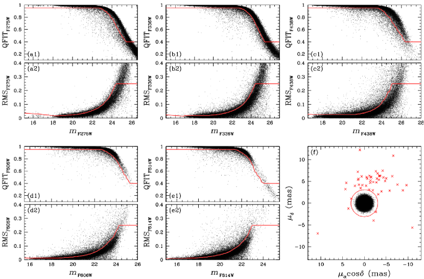
For all five filters, we required a star to have at least two good measurements ($N_{\rm g}$$\geq$2) that are at least 2.5 sigmas above the local sky-background noise. This choice is motivated by the fact that we want to correct DR across the widest possible FoV, but at the same time we want to keep under control the number of poorly-measured stars near the edges of the FoV and minimize false detections (e.g., cosmic rays). We also excluded all those stars for which the $o$ parameter is larger that 1. Then, separately for each filter, we applied two cuts based on the photometric RMS and the QFIT parameter (Fig. 1). To do this, we binned the stars every 0.1 magnitude and computed the 85^th percentile of the photometric RMS and QFIT distributions in each bin. We set three hard constraints: stars are always well-measured if their QFIT values are above 0.95, and are always rejected if their QFIT values are below 0.4 or if their photometric RMS is larger than 0.25 magnitudes.. We then fitted a third-order polynomial to the computed percentile values as a function of the magnitude (red lines in panels a1-2, b1-2, c1-2, d1-2 and e1-2 of Fig. 1) on both the QFIT vs. magnitude and photometric RMS vs. magnitude planes. These lines separate the bulk of well-measured stars from the few clear outliers in each panel. 84 155 stars appeared to be good according to all the selection criteria.

Finally, we required selected stars to be cluster members. Of the 84 155 high-photometric-quality stars, only 72 657 have a measured proper motion. The vast majority of 11,498 stars with no proper-motion measurements are close to the faint magnitude limit (see also Paper I for a description of the proper-motion catalog). In panel (f) of Fig. 1 we show the proper-motion diagram of the 72 657 high-photometric-quality stars. On this panel we defined as cluster members all those stars within the red circle (which radius is arbitrarily defined as 4.2 times the average proper-motion dispersion). The 48 stars outside the red circle, marked with red crosses, are likely field stars.

The final sample contains 72 609 proper-motion selected, well-measured stars in all five filters, homogeneously displaced in a roughly square region of about $4\farcm 3$$\times$$4\farcm 3$ around the cluster’s center.

2.3. Reference Stars

As mentioned above, we prefer to use as reference stars a large number of objects belonging to a single stellar population, and in a region of the CMD where the sequence of this population is as perpendicular as possible to the direction of the reddening vector.

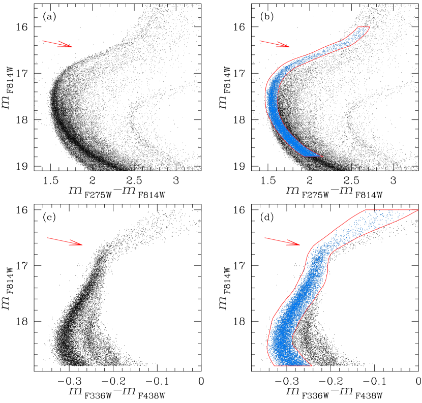
The most-populated sequence of $\omega$Cen around the SGB region is easily recognizable as the brighter branch on the $m_{\rm F814W}$ vs. $m_{\rm F275W}-m_{\rm F814W}$ CMD (panel (a) of Fig. 2). Stars belonging to this sequence are the progeny of red MS stars. The red arrow (here and in the other panels of the figure) marks the direction of the reddening vector, which is almost perpendicular to the turn-off/SGB regions. Clearly, stars around the turn-off, SGB and upper MS regions are the best reference-star candidates.

On this CMD we initially selected our reference-star sample by hand (panel (b), red outline), by choosing all objects likely belonging to the most-populated sequence. We limited reference stars to be within the magnitude range 16$\leq$$m_{\rm F814W}$$\leq$18.8. At fainter magnitudes, the MS of this population bends progressively to become almost parallel to the reddening vector, and therefore fainter MS stars do not help us in correcting for DR effects. On the other hand, the inclusion of brighter stars would have made little to no difference, given the scarcity of RGB stars with respect to the much more numerous MS stars.

Now, it is well known that the different populations in $\omega$Cen overlap each other around the turn-off region, with the red MS mostly evolving into the bright SGB and bluer RGB branches, while the progeny of the blue MS mostly populates fainter SGB and redder RGB branches (see, e.g., Bellini et al. 2010). We can clearly notice the blue-MS/red-MS flipping around the turn-off region also in panel (a) of Fig. 2. As a result, our preliminary reference-star selection necessarily includes objects actually belonging to different stellar populations.

In Bellini et al. (2010) we showed that the blue and the red MSs switch their relative position on a CMD based on the $m_{\rm F336W}-m_{\rm F438W}$ color. Panel (c) of Fig. 2 shows the $m_{\rm F814W}$ vs. $m_{\rm F336W}-m_{\rm F438W}$ CMD around the turn-off region for the stars selected in panel (b). It is clear from the figure that our preliminary selection encompasses more than one population of stars, especially below the turn-off level ($m_{\rm F814W}$$\sim$17.5). We improved our reference-star sample (panel d) by keeping only those stars (in azure) within the red outline drawn by hand.

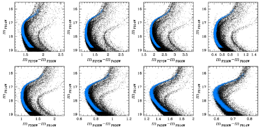
A small fraction of contaminants might still be present in our reference-star sample (e.g., stars belonging to different subpopulations). We explored the possibility of further refining our list of reference stars by plotting them in all the CMDs and two-color diagrams made available by our five adopted filters. The reference stars selected in panel (d) of Fig. 2 define a single sequence in all cases, without any obvious hint of a split or clear contamination from other populations. Therefore, we considered our reference-star list defined in panel (d) as the final sample, which contains 11 655 stars.

2.4. Choosing the Appropriate Correction Plane

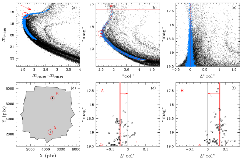
Because the reddening vector’s direction is diagonal with respect to the axes in a CMD, both the magnitude and the color of stars have to be corrected for the effects of DR. If we rotate the CMD in such a way that the reddening vector is parallel to one of the axes, then we have to correct only along one direction, thus simplifying the process. As an example, in panel (a) of Fig. 4 we show the $m_{\rm F438W}$ vs. $m_{\rm F275W}-m_{\rm F814W}$ CMD, in which reference stars are highlighted in azure and the reddening vector is marked in red. We chose an arbitrary rotation point (red encircled dot), and we rotated the CMD counterclockwise by the angle

$$\alpha=\arctan\left(\frac{{\rm A}_{\rm F438W}}{{\rm A}_{\rm F275W}-{\rm A}_{\rm F814W}}\right).$$

The resulting rotated pseudo-CMD is in panel (b), zoomed-in around the SGB. We call the X and Y coordinates of this plane as “col” and “mag”, respectively. For completeness, panel (b) also shows the rotated direction of the reddening vector (red arrow), which is now parallel to the “col” axis, as well as the location of the rotation point.

To further simplify the DR-correction process, we rectified the pseudo-CMD as follows. We computed a fiducial line for the reference-star sequence by least-squares fitting a 5th order polynomial to the “col” and “mag” values of its stars (red curve in panel b). Then, we subtracted from the pseudo-color of each star that of the fiducial line at the same “mag” level. With a rectified reference-star sequence, we can better monitor the following steps of the DR-correction process. The resulting rectified pseudo-CMD is shown in panel (c). Let us call $\Delta$“col” the abscissa of this panel. In order to have an even distribution of reference stars around the fiducial line at any given “mag” level –and therefore avoid any correction bias at the faint and/or the bright end during the next correction steps– we excluded those reference stars (in gray) outside the two red horizontal lines in panel (b).

On a side note, it is worth noting that most of the other SGB branches are tilted with respect to the direction of the rectified reference-star fiducial sequence (panel c). Most of the stars in tilted SGBs that overlap the reference-star sequence are the progeny of the blue MS. The “tilt” is due to a difference in chemical abundances between blue and red MS stars. It is also worth noting that some SGB sequences are more tilted than others. We will return and focus on the multiple stellar populations along the SGB of $\omega$Cen in a future paper of this series.

2.5. Local Corrections

For each star in the catalog (hereafter, the target star), we identify the spatially-closest 75 reference stars, which are used to compute their 2.5-$\sigma$-clipped $\Delta$“col” median value. If the target star also happens to be in the reference list, then the star itself is not used to compute the $\Delta$“col” median value. Panel (d) of Fig. 4 shows the outline of the FoV of our data set, in which we marked the position of two target stars: A and B. The closest 75 reference stars to A and B are found within the two red circles of radius 254.6 and 321.2 pixels, respectively (or about 10$\farcs$2 and 12$\farcs$8).

Panels (e) and (f) of Fig. 4 show the $\Delta$“col” values of the closest 75 reference stars to A and B, respectively. The 2.5$\sigma$-clipped median $\Delta$“col” value in both panels is marked by a red vertical line, while red crosses are rejected stars. The DR correction (for the rotated pseudo-CMD) to be applied to target stars A and B is the opposite of these median $\Delta$“col” (red arrows in panels e and f). The error associated to the DR correction of stars A and B is given by the error of the mean of the associated reference-star median $\Delta$“col” values. For both target stars in the example, we have a correction error of about 0.0042 $\Delta$“col” magnitudes (or about 10% and 6% the applied correction for A and B, respectively), which translates into a CMD color and magnitude error of about 0.003 magnitudes.

Once we have corrected all stars in the catalog on the rotated pseudo-CMD, we can rotate the pseudo-CMD back by the angle $-\alpha$, to obtain the properly DR-corrected CMD.

2.6. Iteration

The DR-corrected CMDs that we have created allow us to fine-tune our original reference-star selections, because on them it is easier to discriminate between stars belonging to the most-populated sequence from the other populations.

We started from the same color-magnitude planes shown in Fig. 2, this time using DR-corrected photometry, and we improved the selection of reference stars by slightly narrowing the color width of the boxes shown in Fig. 2. Moreover, thanks to the DR-corrected photometry, we realized that the selected reference-star sequence splits into 2 branches for magnitudes $m_{\rm F814W}<16.5$ (see, e.g., panel d of Fig. 2 for a reference), therefore we limited reference stars to be fainter than this brightness limit. The improved reference-star list contains 9051 objects.

At this point, we started an iteration process that consists of two steps: 1) we repeated the DR-correction procedures described in the previous subsection; and 2) we improved the list of reference stars using the resulting DR-corrected CMDs. During the iteration procedures, we kept fixed the selection boxes used to define the reference-star sample. Note that the DR-correction is always computed using the raw, uncorrected photometry. What changes from one iteration to the other is the number of reference stars.

After the third iteration, the sequences on the DR-corrected CMDs were negligibly narrower than those after the second iteration, and the number of improved reference stars for an additional, fourth iteration changed only by less than 0.1%. Thus, we did not iterate the DR-correction further, and we considered the results of the third iteration as our final correction.

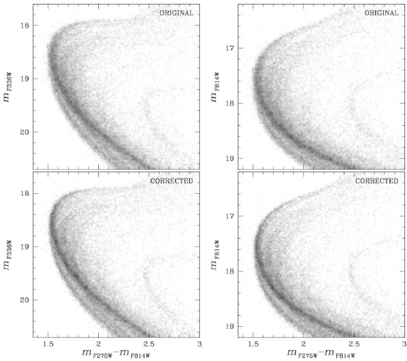
In Fig. 5 we show the Hess diagrams of two of the five CMDs used in this analysis around the SGB region before (top) and after (bottom) the DR-correction is applied, as a demonstration of the effectiveness of the method. The Hess diagrams based on the $m_{\rm F336W}$ vs. $m_{\rm F275W}-m_{\rm F814W}$ CMDs are on the left, the Hess diagrams based on the $m_{\rm F814W}$ vs. $m_{\rm F275W}-m_{\rm F814W}$ CMDs are on the right. The multiple-population sequences in the bottom panels are narrower after the correction, and finer details of SGB and MS substructures are now visible.

Figure 7.— Star-to-star comparison of the filter-based DR-correction values versus the median DR-correction. The red line in each panel is the bisector of the plane (1:1 correlation) and not a fit to the points. The inset in each panel shows the distribution of the points in the direction orthogonal to the red line, which provides an estimate of the internal errors.

3. Reddening-Map Analysis

One of the by-products of our DR-correction procedures is a DR map of the field. As briefly mentioned at the beginning of the previous Section, in principle our corrections account for both DR and photometric zero-point variations across the FoV. If the contribution of the latter is significant, then we should expect sizable differences between DR maps obtained from different CMDs. If there are marginal variations. that would imply that the high-precision PSF models we used are also highly accurate. The comparison of DR maps based on different CMDs thus represents a powerful diagnostic tool for the characterization of the quality of our PSF models.

The DR maps based on the 5 CMDs are constructed as follows. First, we considered only the component of the DR correction along the Y axis, which is the only axis that changes from one CMD to another (being the $m_{\rm F275W}-m_{\rm F814W}$ color fixed in all five CMDs). Let us consider the $m_{\rm F275W}$ vs. $m_{\rm F275W}-m_{\rm F814W}$ CMD as a guideline. For a given star, its DR-corrected $m_{\rm F275W}^{\rm CORR}$ magnitude is obtained as:

$$m_{\rm F275W}^{\rm CORR}=m_{\rm F275W}^{\rm RAW}-\frac{{\rm A}_{\rm F275W}}{{\rm E}(B-V)}\delta{\rm E}(B-V)_{\rm F275W},$$

where $\delta{\rm E}(B-V)_{\rm F275W}$ is the applied DR value in magnitudes, and $m_{\rm F275W}^{\rm RAW}$ is the stellar raw, uncorrected magnitude. Using the appropriate extinction-coefficient value for the F275W filter listed in Table 1, it follows:

$$\delta{\rm E}(B-V)_{\rm F275W}=\frac{m_{\rm F275W}^{\rm RAW}-m_{\rm F275W}^{\rm CORR}}{6.10379}.$$

For each star we can compute five independent DR values, one for each of the five filters.

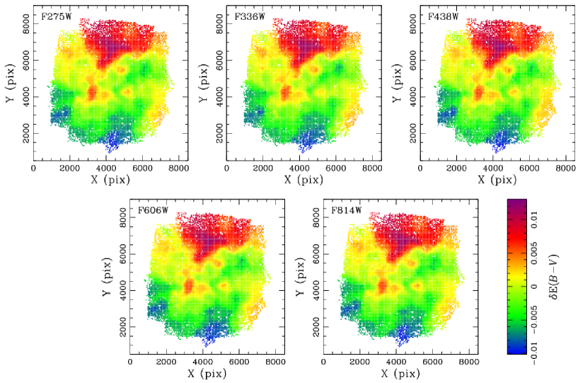
The values $\delta{\rm E}(B-V)_{\rm filter}$ as a function of the (X,Y) stellar position can be used to construct two-dimensional maps of the DR across the FoV. The five panels in Fig. 6 show these maps, one for each of the five filters (listed in the top-left corner of each panel). The panels adopt the same color mapping, the scale of which is shown in the bottom-right part of the figure. These five maps look remarkably similar to each other, both in shape and intensity. This means that our carefully-modeled PSFs (see Paper I, Section 3.1), together with the availability of a large number of dithered exposures with different roll angles, were able to minimize the effects of photometric zero-point residuals.

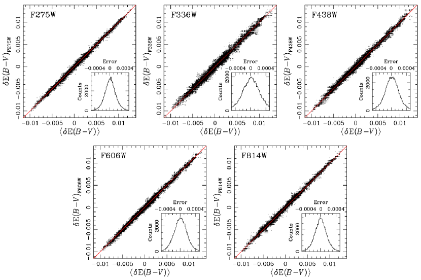
For each star we compared the five $\delta{\rm E}(B-V)_{\rm filter}$ values we obtained with respect to their median value $\langle\delta{\rm E}(B-V)\rangle$, which represents our best estimate of the true DR for that star (Fig. 7). The red line in each panel is the bisector of the plane and not a fit to the points. Each panel reveals the presence of small systematic deviations from the 1:1 correlation, especially at the extremes of distribution, and in particular for the $\delta{\rm E}(B-V)_{\rm F336W}$ and $\delta{\rm E}(B-V)_{\rm F438W}$ values. Nonetheless, the fact that in all cases the points are nicely aligned along the red line represents a clear validation of our technique. We least-squares-fitted a straight line to the unweighted points in each panel, and the slopes we obtained are indeed very close to the value of 1 (see Table 1, third column).

Table 1
Filter-based DR Comparison
Filter	Afilter/E($B-V$)	Slope	$\sigma$
F275W	6.10379	1.00102$\pm$0.00018	0.00014
F336W	5.04267	0.99853$\pm$0.00036	0.00022
F438W	4.04616	0.99502$\pm$0.00027	0.00018
F606W	2.62074	1.00091$\pm$0.00023	0.00017
F814W	1.64912	1.00089$\pm$0.00010	0.00015

In each panel, the dispersion of the points orthogonal to the red line gives us an independent estimate of the internal errors. A histogram of the distribution of these orthogonal dispersions is shown in the inset of each panel. A Gaussian fit to these histograms provides a first-guess estimate of the internal errors, which are found to be smaller than 2$\times$10^-4 mag in all five cases. The $\sigma$ of the fitted Gaussians are reported in the fourth column of Table 1. A somewhat larger $\sigma$ for the F336W filter might suggest that our PSF models for this filter were not as fine-tuned as for the other filters.

Figure 8.— Top panel: the final DR map of the core of $\omega$Cen, shown in the rectified Cartesian plane with respect to the cluster’s center. Bottom left: The local semi-interquartile (SIQ) values of the five filter-dependent DR maps across the FoV. Bottom right: a map of how far from the center of each 50$\times$50 pixels² 75 reference stars are found (1 pixel = 40 mas). The color-coding of each panel is shown to its right side.

Now, a more careful look at the values of the slopes we obtain reveals that some of these values are significantly different from 1 (especially for the F438W filter), even if we take into account both the error of the slope and the $\sigma$ of the Gaussian fit. At first, we thought that we could take advantage of these results and attempt to recover both the true DR map and the true extinction curve from our data set. We tried to iterate the DR-correction procedures by adjusting each time the extinction coefficients in such a way as to have the five slopes in Fig. 7 identically equal to 1: A${}_{\rm filter}^{\rm new}$=A${}_{\rm filter}^{\rm orig}/{\rm slope}$, but the improved values of the slopes that we obtained after each iteration kept oscillating around their initial values and never converged to unity as we would have hoped.

Then, we realized that we are actually facing a double-degenerate problem. For each of the five CMDs, the only things we know observationally are the location of the reference-star fiducial line and the location of the target stars. We do not know the true value of the extinction coefficients, but only their estimate. In addition, we do not know the true DR affecting each target star, but only an estimate. Finally, we also do not know the true position of the reference stars on the $\Delta$“col” plane as they would appear at the average reddening of the cluster, but only that these stars must be on the fiducial line. For a given reference star, there are a total of 7 unknown quantities, namely: its true DR, its true position on the $\Delta$“col” plane, and the true value of the extinction coefficients.

Regardless of the number of filters $M$ we use to solve for the DR, there will always be $M+2$ unknowns. Hence, there is a 2-parameter family of solutions. One degeneracy arises from the fact that only combinations of A_filter$\times$$\delta$E($B$$-$$V$)_filter are observable, therefore there is a multiplicative degeneracy between the true DR values $\delta$E($B$$-$$V$)_filter and the extinction coefficients A_filter. A second degeneracy arises from the fact that we do not know where a reference star really lies with respect to the reference-star fiducial line.

Given these degeneracies, we cannot determine the DR and the extinction curve simultaneously. The approach we take in this paper is to assume that we know the value of the extinction coefficients, and we then determine the DR. This approach yields a unique solution, which is in fact what we encounter. The slope values in Table 1 indicate that different CMDs imply a (slightly) different differential reddening. This means that the adopted Fitzpatrick (1999) extinction curve is not consistent with our data at the $\sim$0.1% level. However, the fact that the slope values in Table 1 are so close to unity indicates that the uncertainty in our DR maps due to uncertainties in the extinction coefficients are very small. In principle, the results can be improved by changing the assumed extinction curve. However, there is no unique way of doing this, since there is a two-parameter family of solutions. Hence, an iterative approach such as the one we tried does not converge.

3.1. The Final Differential-Reddening Map

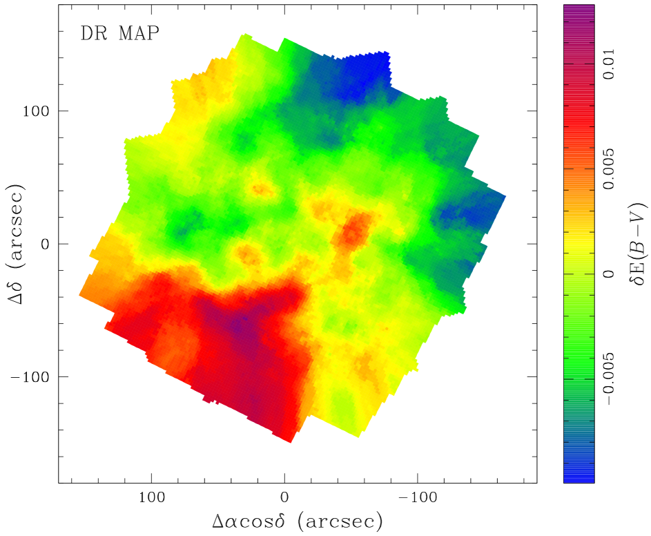
The top panel of Fig. 8 shows our final, $\langle\delta{\rm E}(B-V)\rangle$ map, in the rectified Cartesian (R.A.,Dec.) plane, in units of arcseconds with respect to the cluster’s center. This map represents our best estimate of the real DR in the field. To create the map, we sampled the available FoV every 50$\times$50 pixel² (i.e., 2$\times$2 arcsec²), and we applied to each of these 2500 pixels the median value of the five filter-dependent DR corrections computed at the center of the cell. A 50$\times$50-pixel² sampling provides for a smooth representation of the DR map, and largely supersamples the typical resolution of our DR-correction (given that, on average the closest 75 reference stars to a given target star are found within 330 pixels, or 13^′′).

The map has an average value of zero across the entire field (the size of which is approximately $4\farcm 3$$\times$$4\farcm 3$), since we computed the DR with respect to the average reddening of the field.

Overall, the DR values on the map have a standard deviation of 0.005 ${\rm E}(B-V)$ magnitudes. Minimum and maximum ${\rm E}(B-V)$ values are $-$0.010 and +0.013 magnitudes, respectively, which (assuming an average ${\rm E}(B-V)$=0.12 magnitudes) translate into a typical DR variation of 4%, and up to about $\pm$10% (at most) the average reddening. Another way to read these results is that the DR in the core of $\omega$Cen can vary by up to 20% (minimum to maximum).

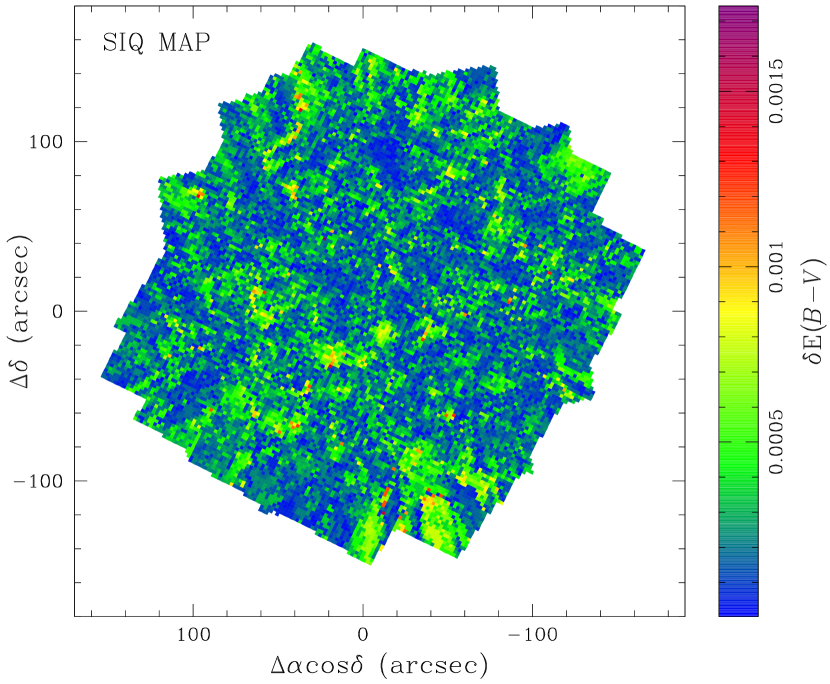
The bottom-left panel of the figure shows a map of the semi-interquartile (SIQ) of the five filter-based $\delta{\rm E}(B-V)$ values at each of the 50$\times$50 pixel² locations, shown in the same rectified Cartesian plane as the top-panel map. The SIQ provides an estimate of the local scatter between the five DR estimates. Overall, the SIQ-value distribution is flat across the FoV, with typical variations of the order of 0.0003 ${\rm E}(B-V)$ (less than 10% the DR standard deviation). There are a few localized regions, mostly close to the edges of the FoV where we have only a few (typically two) exposures per filter, or in close proximity of oversaturated stars in some filters, in which the SIQ is as high as 0.0016 ${\rm E}(B-V)$.

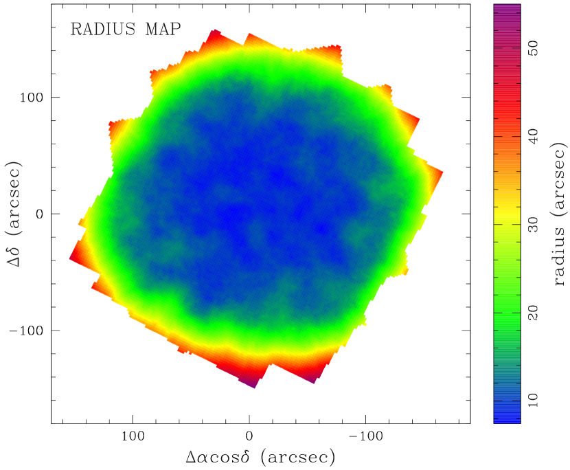
Finally, the bottom-right panel shows the rectified Cartesian map of the typical values of the radius within which 75 reference stars are found for each of the 50$\times$50 pixel² locations. The color-mapping scale is in pixel units. Given the WFC3/UVIS pixel scale of 40 mas pixel^-1, the minimum and maximum values are 10^′′ and 43^′′, respectively. Clearly, the DR map is less constrained near the corners of the FoV, where 75 reference stars are found only along one direction (toward the center of the FoV).

Figure 9.— The DIRBE/IRAS reddening map in the direction of $\omega$Cen (Schlegel et al. 1998), adapted from (van Loon et al., 2009, their Fig. 10b). The cluster’s center is marked by a white cross. The outline of our FoV is in red. The gray-scale intensity of the map ranges from E($B-V$)=0.144 mag (dark) to 0.124 mag (light).

4. Discussion and Conclusions

In this paper, we took advantage of the exquisite astro-photometric catalog we constructed in Paper I to derive a high-precision DR map of the core of the globular cluster $\omega$Cen. The DR is estimated using five CMDs based on the following UVIS filters: F275W, F336W, F438W, F606W and F814W. There are at least 34 single exposures taken through each of these filters, with different roll angles and dither patterns, so that the impact of PSF-related, zero-point spatial variations across the field is minimized to the extent possible. In addition, images taken through these filters cover the widest available FoV around the cluster’s core.

The five independent solutions for the DR we found agree very well with each other, with typical semi-interquartile values of 0.0003 ${\rm E}(B-V)$. The median of the five DR maps constitutes our best estimate of the true DR around the core of the cluster. Within our FoV (about $4\farcm 3$$\times$$4\farcm 3$) the DR has standard deviation, minimum and maximum values of 0.005 mag, $-$0.010 mag and 0.013 mag in terms of ${\rm E}(B-V)$, respectively. Assuming an average reddening of E($B-V$)=0.12 (Harris 1996), these values translate into a typical DR variation of about only 4%, and up to $\sim$$\pm$10% at the extremes.

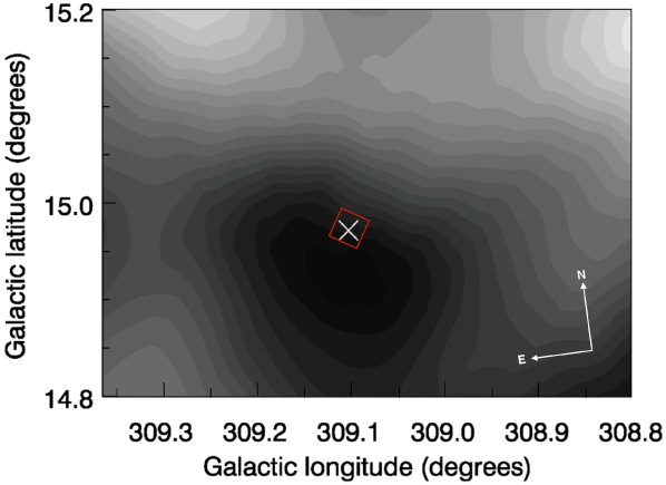
Our findings are consistent with the qualitative analysis of Villanova et al. (2007), but are in sharp contrast with the results of Calamida et al. (2005), who found clumpy reddening variations of almost a factor of two (minimum to maximum) within the cluster’s core. In addition, Calamida et al. (2005) found that the greatest density of more highly-reddened objects is shifted along the right ascension axis when compared with less reddened ones. Our DR map, on the other hand (top panel of Fig. 8), shows that the regions with the highest and lowest DR are the South-East and the North-West quadrants, respectively. Both direction and orientation of the DR gradient we find are qualitatively consistent with the DIRBE/IRAS reddening map of the region compiled by Schlegel et al. (1998). In Fig. 9 we show a portion of this DIRBE/IRAS map, adapted from van Loon et al. (2009, their Fig. 10). The footprint of our FoV is highlighted in red, while the cluster’s center is marked by a white cross. The Schlegel et al. (1998) DR map, despite having a much lower spatial resolution than ours, clearly suggests a DR gradient (high to low) from the South-East to the North-West with respect to the cluster’s center within our FoV.

A possible explanation of the differences between the Calamida et al. (2005) DR analysis and both the DIRBE/IRAS DR map and the DR map presented here is that Calamida et al. (2005) treated the horizontal branch of $\omega$Cen as if it were the result of the evolution of a “single stellar population”, i.e., stars born at the same time and with the same chemical composition. It has been known for a long time that $\omega$Cen hosts stars with a wide range in metallicity (e.g., Cannon & Stobie 1973), and more recently that it also hosts distinct stellar populations in all evolutionary sequences (e.g, Anderson 1997; Lee et al. 1999; Bedin et al. 2004). More importantly, stars in $\omega$Cen exhibit a large spread in helium content (e.g., Norris 2004; Piotto et al. 2005; King et al. 2012): a spread that plays a major role in shaping the blue-horizontal-branch morphology (see, e.g., D’Antona & Caloi 2004, 2008).

We release to the astronomical community our high-resolution, high-precision, and high-accuracy DR map in the form of a multi-extension FITS file containing the three maps shown in Fig. 8. The DR map itself is in the first extension. The second extension contains the SIQ map, while the values of the local-averaged radius (in pixels) within which 75 reference stars are found are in the third extension.

References

- Anderson (1997) Anderson, J., Ph.D. thesis, Univ. of California, Berkeley, 1997
- Bedin et al. (2004) Bedin, L. R., Piotto, G., Anderson, J., et al. 2004, ApJ, 605, L125
- Bellini et al. (2010) Bellini, A., Bedin, L. R., Piotto, G., et al. 2010, AJ, 140, 631
- Bellini et al. (2013) Bellini, A., Piotto, G., Milone, A. P., et al. 2013, ApJ, 765, 32
- Bellini et al. (2016) Bellini, A., Anderson, J., Bedin, L. R., et al. 2016, submitted to ApJ
- Calamida et al. (2005) Calamida, A., Stetson, P. B., Bono, G., et al. 2005, ApJ, 634, L69
- Cannon & Stobie (1973) Cannon, R. D., & Stobie, R. S. 1973, MNRAS, 162, 207
- Cleveland (1979) Cleveland, W. S. 1979, Journal of the American Statistical Association, 74, 829–836
- D’Antona & Caloi (2004) D’Antona, F., & Caloi, V. 2004, ApJ, 611, 871
- D’Antona & Caloi (2008) D’Antona, F., & Caloi, V. 2008, MNRAS, 390, 693
- D’Souza & Rix (2013) D’Souza, R., & Rix, H.-W. 2013, MNRAS, 429, 1887
- Fitzpatrick (1999) Fitzpatrick, E. L. 1999, PASP, 111, 63
- Harris (1996) Harris, W. E. 1996, AJ, 112, 1487 (2010 edition)
- King et al. (2012) King, I. R., Bedin, L. R., Cassisi, S., et al. 2012, AJ, 144, 5
- Krige (1951) Krige, D. G. 1951, Master’s thesis, University of Witwatersrand
- Lee et al. (1999) Lee, Y.-W., Joo, J.-M., Sohn, Y.-J., et al. 1999, Nature, 402, 55
- Marino et al. (2011) Marino, A. F., Milone, A. P., Piotto, G., et al. 2011, ApJ, 731, 64
- Milone et al. (2012) Milone, A. P., Piotto, G., Bedin, L. R., et al. 2012, A&A, 540, A16
- Nadaraya (1964) Nadaraya, E. A. 1964, Theory of Probab. Appl., 9(1): 141-142
- Norris (2004) Norris, J. E. 2004, ApJ, 612, L25
- Piotto et al. (2005) Piotto, G., Villanova, S., Bedin, L. R., et al. 2005, ApJ, 621, 777
- Piotto et al. (2015) Piotto, G., Milone, A. P., Bedin, L. R., et al. 2015, AJ, 149, 91
- Schlegel et al. (1998) Schlegel, D. J., Finkbeiner, D. P., & Davis, M. 1998, ApJ, 500, 525
- Silverman (1984) Silverman, B. W. 1984, Journal of the American Statistical Association, 79, 584–589
- van Loon et al. (2009) van Loon, J. T., Smith, K. T., McDonald, I., et al. 2009, MNRAS, 399, 195
- Villanova et al. (2007) Villanova, S., Piotto, G., King, I. R., et al. 2007, ApJ, 663, 296
- Villanova et al. (2014) Villanova, S., Geisler, D., Gratton, R. G., & Cassisi, S. 2014, ApJ, 791, 107
- Watson (1964) Watson, G. S. 1964, Sankhyā: The Indian Journal of Statistics, Series A, 26(4): 359–372