1 Introduction

Accurate calculation of the $B\to\pi$ transition form factors in QCD plays an important role, since, for instance, the vector form factor is used for the determination of the Cabibbo-Kobayashi-Maskawa (CKM) matrix element $V_{ub}$ from the experimental data on the exclusive $B\to\pi\ell\nu_{\ell}$ decays. The $B\to\pi$ transition form factors are nonperturbative quantities accounting for the complicated quark-gluon dynamics inside the meson states and can be calculated using different QCD-based approaches. Among them, the method of light cone sum rules (LCSR) [1, 2] is applicable at large hadronic recoil [3, 4]. The main advantage of this method is the possibility to perform calculation in full QCD, with finite $b$-quark mass. The starting object of the calculation is a properly designed correlation function of the quark currents for which the operator product expansion (OPE) near the light-cone is applicable. Within OPE, the correlation function is decomposed into a series of the hard-scattering kernels convoluted with the pion light-cone distribution amplitudes (DA’s) of the growing twist. The result of the OPE for correlation function is related to the $B\to\pi$ form factor employing the hadronic dispersion relation and quark-hadron duality.

At present time the accuracy of the LCSR calculation of heavy-to-light transition form factors is limited by the contributions of the operators up to twist 4. The results for the relevant partial contributions of the twist-2, -3 and -4 terms to the LCSR as well as radiative gluon corrections to the corresponding hard-scattering kernels of the twist-2 and twist-3 terms can be found in [3, 4, 5, 6, 7, 8]. Moreover, a $\beta_{0}$ estimation for the twist-2 $O(\alpha_{s}^{2})$ contributions can be found in [9]. It is important to note that the contributions of even- and odd-twist terms in the OPE form two separate hierarchies with respect to the lowest twist-2 and twist-3 terms, respectively. Note also that the twist-3 term, despite power suppression, contains a chirally enhanced parameter $\mu_{\pi}=m_{\pi}^{2}/(m_{u}+m_{d})$, which renders the twist-3 contribution to the same order of magnitude as the twist-2 one. The contribution of twist-4 term was found to be significantly suppressed in comparison with the corresponding twist-2 one [5]. Such a comparison in the odd-twist hierarchy is still not possible due to missing estimate of twist-5 effects. Moreover, an estimate of the twist-6 term contribution to LCSR will allow us to confirm the expected power suppression of the higher twists in the even-twist hierarchy. The main purpose of this work is to evaluate the twist-5 and twist-6 contributions to the LCSR for the $B\to\pi$ form factors.

The calculation of the higher twist effects in the OPE near the light-cone is interesting for several reasons. As mentioned in Ref. [11], the twist-3 and twist-4 operators cannot be factorized as a product of the gauge invariant operators of lower twist. There are several operators of twist 5 and twist 6 which can be factorized as a product of the gauge-invariant operators of lower twist. Sandwiched between the vacuum and one-pion state, such operators generally produce two types of contributions: factorizable ones in terms of a lower-twist two-particle distribution amplitude times quark condensate and nonfactorizable ones, which give rise to genuine twist-5 and twist-6 multiparton pion distribution amplitudes. As argued in [11], in the context of conformal symmetry the contributions of higher Fock states are strongly suppressed and their contributions to the sum rules are probably negligible. Factorizable contributions, on the other hand, can be comparatively large. Hence their calculation practically solves the problem of investigating the OPE beyond the twist-4 level.

In [11] and [12] the factorizable twist-6 contributions in LCSR’s for the pion electromagnetic and $\pi\gamma^{*}\gamma$ form factors, respectively, were computed. In fact, in these sum rules the twist-6 contributions are the only ones which arise in the presence of virtual massless ($u$- or $d$)-quark in the correlation function, hence, only the even twists are relevant there. Here we extend the analogous calculation to the correlation function with a massive virtual quark. In this case both factorizable twist-5 and twist-6 terms contribute to LCSR. In order to obtain these contributions one needs the massive quark propagator expanded near the light-cone up to the terms including the derivatives of the gluon field strength. The analytical expression for this propagator as well as the factorizable twist-5 and twist-6 contributions to LCSR represent new results obtained here.

The paper is organised as follows. Sec. 2 is devoted to the derivation of the new terms in the expansion of the massive quark propagating in the external gluonic field near the light-cone. In Sec. 3 the detailed calculation of the diagrams corresponding to the factorizable twist-5 and twist-6 contributions to the LCSR for the vector $B\to\pi$ form factor is presented. Sec. 4 contains the relevant numerical estimates and Sec. 5 the concluding discussion. Some useful formulae are collected in the appendix.

2 Light-cone expansion of the massive quark propagator in the external gluon field

For our purpose we need the light-cone (LC) expansion of the quark propagator in the external gluon field. The corresponding expression including the terms with the covariant derivatives of gluon field strength is known only in the case of massless quark and was derived for instance in [10] (see also [11]). For a massive quark propagator the corresponding result is known only at leading order of the LC-expansion in the gluon field. To estimate the higher twist effects in the $B\to\pi$ form factors we need also to include the higher order terms in LC-expansion which are proportional to the covariant derivatives of the gluon-field strength. This task is technically more involved due to a presence of the quark mass $m$.

In order to get the LC-expansion of the massive quark propagator up to the needed accuracy we start from the definition of the quark propagator:

$$S(x,x^{\prime})=-i\langle 0|T\{\psi(x),\bar{\psi}(x^{\prime})\}|0\rangle,$$ (1)

where $\psi(x)$ denotes the massive quark field operator. Hereafter we choose $x^{\prime}=0$ for simplicity. The propagator satisfies the usual Green-function equation

$$\left(i\gamma^{\mu}\partial_{\mu}+g_{s}\gamma^{\mu}A_{\mu}(x)-m\right)S(x,0)=\delta^{(4)}(x),$$ (2)

where $A_{\mu}=A_{\mu}^{a}\lambda^{a}/2$ is the four-potential of the gluon field, and $\lambda^{a}$ are the Gell-Mann matrices $(a=1,\ldots 8)$. The solution of (2) can be presented in the form of perturbative series in the power of the strong coupling $g_{s}$:

$$iS(x,0)=iS^{(0)}(x)+iS^{(1)}(x)+\ldots$$ (3)

where

$$iS^{(1)}(x)=g_{s}\int d^{4}y\,iS^{(0)}(x-y)\,i\not{A}(y)\,iS^{(0)}(y),$$ (4)

and $S^{(0)}$ denotes the free quark propagator. The four-potential of the gluon field is taken in the Fock-Schwinger (of fixed point) gauge, so that $(x_{\mu}-x^{\prime}_{\mu})A^{\mu}(x)=0$ and $x^{\prime}=0$. For further calculation it is convenient to use the free quark propagator $S^{(0)}(x-y)$ in the form of so-called $\alpha$-representation

$$S^{(0)}(x-y)=-i\int\limits_{0}^{\infty}\frac{d\alpha}{16\pi^{2}\alpha^{2}}\left(m+i\frac{\not{x}-\not{y}}{2\alpha}\right)e^{-m^{2}\alpha+\frac{(x-y)^{2}}{4\alpha}},$$ (5)

which allows us to rewrite the first order correction $S^{(1)}(x,0)$ to the propagator as follows:

$$S^{(1)}(x,0) = \frac{g_{s}}{(16\pi^{2})^{2}}\int\limits_{0}^{\infty}\frac{d\alpha}{\alpha^{2}}\int\limits_{0}^{\infty}\frac{d\beta}{\beta^{2}}\int d^{4}y$$

$$\times \left(m+i\frac{\not{x}-\not{y}}{2\alpha}\right)\not{A}(y)\left(m+i\frac{\not{y}}{2\beta}\right)e^{-m^{2}(\alpha+\beta)}e^{\frac{(x-y)^{2}}{4\alpha}+\frac{y^{2}}{4\beta}}.$$

Transforming the integration variable $\beta$ as:

$$\beta=\frac{\alpha u}{1-u},\quad 0<\beta<\infty\quad\mbox{ so that }\quad 0<u<1,$$ (7)

we introduce a new variable:

$$y^{\prime}=y-ux.$$ (8)

Taking into account the replacements (7) and (8) one can represent the expression (2) in the form (hereafter we redefine $y^{\prime}\to y$):

$$S^{(1)}(x,0)=\frac{g_{s}}{(16\pi^{2})^{2}}\int\limits_{0}^{1}\frac{du}{u^{2}}\int\limits_{0}^{\infty}\frac{d\alpha}{\alpha^{3}}\int d^{4}y\,e^{-m^{2}\alpha/\bar{u}}e^{[y^{2}+x^{2}u\bar{u}]/(4\alpha u)}$$

$$\times \Bigg{\{}m^{2}\not{A}(y+ux)+\frac{im}{2\alpha u}\Big{[}2u\bar{u}(x\cdot A(y+ux))-2u(y\cdot A(y+ux))+\not{A}(y+ux)\not{y}\Big{]}-$$

$$- \frac{\bar{u}}{4\alpha^{2}u}\Big{[}u\bar{u}\not{x}\not{A}(y+ux)\not{x}-u\not{y}\not{A}(y+ux)\not{x}+\bar{u}\not{x}\not{A}(y+ux)\not{y}-\not{y}\not{A}(y+ux)\not{y}\Big{]}\Bigg{\}},$$

where $\bar{u}=1-u$, $(x(y)\cdot A)\equiv x_{\mu}(y_{\mu})A^{\mu}$. After that we expand the field $A_{\alpha}(y+ux)$ in the powers of the deviation $y_{\mu}$ from the point $ux$ near the light cone $(x^{2}\simeq 0)$:

$$A_{\alpha}(y+ux) = A_{\alpha}(ux)+\partial_{\mu}A_{\alpha}(ux)y^{\mu}+\frac{1}{2}\partial_{\mu}\partial_{\nu}A_{\alpha}(ux)y^{\mu}y^{\nu}$$ (10)

$$+ \frac{1}{6}\partial_{\mu}\partial_{\nu}\partial_{\rho}A_{\alpha}(ux)y^{\mu}y^{\nu}y^{\rho}+\ldots,$$

with the following shorthand notation: $\partial_{\mu}A_{\alpha}(ux)\equiv\left.\frac{\partial A_{\alpha}(z)}{\partial z^{\mu}}\right|_{z=ux}.$ Substituting the expansion (10) in (2) allows to calculate $S^{(1)}(x,0)$ order by order. Performing the Wick’s rotation $y_{0}\to-iy_{4}$, one reduces the integrals over $d^{4}y$ to the standard Gaussian integrals. After integration over $d^{4}y$, one calculates the integrals over $\alpha$ introducing the modified Bessel function of the second kind $K_{n}(z)$:

$$\int\limits_{0}^{\infty}\frac{d\alpha}{\alpha^{n}}\,{\rm exp}\left[-\frac{m^{2}\alpha}{1-u}+\frac{x^{2}(1-u)}{4\alpha}\right]=2\left(\frac{2m}{\sqrt{-x^{2}}(1-u)}\right)^{\!\!\frac{n-1}{2}}\!\!\!K_{n-1}(m\sqrt{-x^{2}}),\quad x^{2}<0.$$ (11)

Then we perform some transformations in order to relate the derivatives of $A_{\rho}(xu)$ with $G^{\mu\nu}(ux)$ and its derivatives. The first term in the expansion (10) yields the scalar product $(x\cdot A)$ which vanishes in the Fock-Schwinger gauge. Since $S^{(1)}(x,0)$ has ${\cal O}(g_{s})$ accuracy, the partial derivatives $\partial_{\mu}$ can be replaced by the covariant ones $D_{\mu}$. Taking into account the definition of the gluon-field strength tensor $G_{\mu\nu}=G_{\mu\nu}^{a}\lambda^{a}/2=D_{\mu}A_{\nu}-D_{\nu}A_{\mu}$, one relates then the covariant derivatives of $A_{\mu}$ with $G_{\mu\nu}$ and its derivatives. We found that the terms proportional to $D^{\mu}A_{\mu}$ vanish after integration by parts in variable $u$, allowing one to present the final result for the propagator in terms of gluon-field strength only.

After lengthy but straightforward calculation we arrive at the following expression for the massive quark propagator expanded near the light-cone, including terms up to the second derivative of the gluon field strength:

$$S(x,0) = -\frac{im^{2}}{4\pi^{2}}\left[\frac{K_{1}(m\sqrt{-x^{2}})}{\sqrt{-x^{2}}}+i\frac{\not{x}}{-x^{2}}K_{2}(m\sqrt{-x^{2}})\right]$$

$$- \frac{ig_{s}}{16\pi^{2}}\int\limits_{0}^{1}du\Biggl{[}mK_{0}(m\sqrt{-x^{2}})(G(ux)\cdot\sigma)$$

$$+ \frac{im}{\sqrt{-x^{2}}}K_{1}(m\sqrt{-x^{2}})\left[\bar{u}\not{x}(G(ux)\cdot\sigma)+u(G(ux)\cdot\sigma)\not{x}\right]$$

$$- 2u\bar{u}\left(imK_{0}(m\sqrt{-x^{2}})-\frac{m\not{x}}{\sqrt{-x^{2}}}K_{1}(m\sqrt{-x^{2}})\right)x_{\mu}D_{\nu}G^{\nu\mu}(ux)$$

$$+ K_{0}(m\sqrt{-x^{2}})\left(2u\bar{u}-1\right)\gamma_{\mu}D_{\nu}G^{\nu\mu}(ux)$$

$$- u\bar{u}(1-2u)K_{0}(m\sqrt{-x^{2}})x_{\mu}\not{D}D_{\nu}G^{\nu\mu}(ux)$$

$$- iu\bar{u}K_{0}(m\sqrt{-x^{2}})\epsilon_{\sigma\mu\nu\rho}x^{\sigma}\gamma^{\mu}\gamma_{5}D^{\nu}D_{\alpha}G^{\alpha\rho}(ux)$$

$$+ u\bar{u}\sqrt{-x^{2}}K_{1}(m\sqrt{-x^{2}})\sigma_{\rho}^{\phantom{\rho}\nu}D_{\nu}D_{\mu}G^{\mu\rho}(ux)\Biggr{]}+\ldots$$

where $(G\cdot\sigma)\equiv G_{\mu\nu}\sigma^{\mu\nu},\,\sigma^{\mu\nu}=(i/2)[\gamma^{\mu},\gamma^{\nu}]$, and dots denote the higher powers of the light-cone expansion of $G_{\mu\nu}$ and corrections with two and more gluons, which are beyond the approximation we need. Taking into account the asymptotics of the Bessel functions:

$$\left.K_{0}(m\sqrt{-x^{2}})\right|_{m\to 0} \sim -\gamma_{E}-\ln\left(\frac{m}{2}\right)-\frac{1}{2}\ln\left(-x^{2}\right),$$

$$\left.\sqrt{-x^{2}}K_{1}(m\sqrt{-x^{2}})\right|_{m\to 0} \sim \frac{1}{m},$$ (13)

one reproduces the corresponding result in the case of the massless quark given in [10, 11].

We also found that the resulting expression (2) can be rewritten in an equivalent Fourier-transformed form:

$$S(x,0) = \int\frac{d^{4}p}{(2\pi)^{4}}e^{-ipx}\Biggl{\{}\frac{\not{p}+m}{p^{2}-m^{2}}-\frac{g_{s}}{\left(p^{2}-m^{2}\right)^{3}}\int\limits_{0}^{1}du\biggl{[}\frac{1}{2}m(p^{2}-m^{2})(G(ux)\cdot\sigma)+$$ (14)

$$+ \frac{1}{2}(p^{2}-m^{2})\left(\bar{u}\not{p}(G(ux)\cdot\sigma)+u(G(ux)\cdot\sigma)\not{p}\right)-4u\bar{u}(\not{p}+m)p_{\mu}D_{\nu}G^{\nu\mu}(ux)-$$

$$- \frac{1}{2}(p^{2}-m^{2})\gamma_{\mu}D_{\nu}G^{\nu\mu}(ux)-2iu\bar{u}(1-2u)p_{\mu}\not{D}D_{\nu}G^{\nu\mu}(ux)+$$

$$+ 2u\bar{u}\epsilon_{\sigma\mu\nu\rho}p^{\sigma}\gamma^{\mu}\gamma_{5}D^{\nu}D_{\alpha}G^{\alpha\rho}(ux)-2mu\bar{u}\sigma_{\rho}^{\phantom{\rho}\nu}D_{\nu}D_{\mu}G^{\mu\rho}(ux)+\ldots\biggr{]}\Biggr{\}}.$$

The first terms of this expression are in full agreement with the LC-expansion of the massive quark propagator given in [4], and the terms with the covariant derivative of the gluon field strength represent a new result of this paper.

3 Factorizable twist-5 and twist-6 contributions to the $B\leavevmode\nobreak\ \to\leavevmode\nobreak\ \pi$ form factor

The starting object for a calculation of the $B\to\pi$ form factors in the framework of the LCSR approach is the following correlation function of the $B$-meson interpolating and the $b\to u$ weak transition currents:

$$F_{\mu}(p,q) = i\int\!d^{4}x\,e^{iqx}\langle\pi(p)|T\{\bar{u}(x)\gamma_{\mu}b(x),m_{b}\bar{b}(0)i\gamma_{5}d(0)\}|0\rangle$$ (15)

$$= F(q^{2},(p+q)^{2})p_{\mu}+\tilde{F}(q^{2},(p+q)^{2})q_{\mu},$$

where $p$ is the four-momentum of the pion, $q$ is the outgoing four-momentum, and $m_{b}$ is the $b$-quark mass. For definiteness, we consider the $\bar{B}_{d}^{0}\to\pi^{+}$ flavour configuration. The Lorentz-invariant amplitudes $F(q^{2},(p+q)^{2})$ and $\tilde{F}(q^{2},(p+q)^{2})$ are used for the calculation of the vector and scalar form factors. In this paper we focus on an estimate of the higher twist effects for the vector form factor, hence, we need to consider only the amplitude $F(q^{2},(p+q)^{2})$. In the framework of LCSR approach one considers the correlation function (15) in the kinematic domain $q^{2}\ll m_{b}^{2}$ and $(p+q)^{2}\ll m_{b}^{2}$, far from the $b$-flavour threshold. In this domain the separations near the light-cone dominate and one can expand the integrand in (15) near $x^{2}=0$ (see e.g. [5]). Contracting the virtual $b$-quark fields one rewrites (15) in the form

$$F_{\mu}(p,q)=-m_{b}\int d^{4}x\,e^{iqx}\langle\pi(p)|\bar{u}(x)\gamma_{\mu}iS_{b}(x,0)\gamma_{5}d(0)|0\rangle,$$ (16)

where $S_{b}(x,0)$ denotes the $b$-quark propagator expanded near the light-cone.

Currently, the accuracy of the OPE for the correlation function at leading order in $\alpha_{s}$ is limited by contributions up to twist-4 terms. In our paper, we focus on a derivation of the factorizable twist-5 and twist-6 contributions. To this end, we substitute the LC-expansion of the $b$-quark propagator calculated in the previous section (see eq. (2)) and take only terms proportional to the derivative $D_{\mu}G^{\mu\nu}$ of the gluon-field strength. The latter are transformed by applying the equation of motion for the gluon-field strength:

$$D_{\mu}G^{\mu\nu}(ux)=-g_{s}\sum_{q}\left(\bar{q}(ux)\gamma^{\nu}\frac{\lambda^{a}}{2}q(ux)\right)\frac{\lambda^{a}}{2}.$$ (17)

In the above, due to the quark content of the final state pion, only the terms with $u$ and $d$-quark contribute. Applying the equation of motion (17) yields the matrix elements of two quark-antiquark operators sandwiched between pion and vacuum states. These matrix elements generate two different types of contributions. The first ones related to the four-particle DAs are expected to be negligible [11]. On the other hand, the contributions of the second type (factorizable) could have larger numerical impact on LCSR for the form factor. In this paper following the same approach as in [11, 12] we restrict ourselves by the factorization approximation and present the matrix elements of the two quark-antiquark operators as a product of the dimension-three quark condensate $\langle\bar{q}q\rangle$ and the bilocal vacuum-pion matrix element containing pion twist-2 and twist-3 light-cone distribution amplitudes (LCDA’s). The latter matrix element can be presented in the form [5]:

$$\langle\pi(p)|\bar{u}_{\alpha}^{i}(x_{1})d_{\beta}^{j}(x_{2})|0\rangle\Big{|}_{(x_{1}-x_{2})^{2}\to 0} = \frac{i\delta^{ij}f_{\pi}}{12}\int\limits_{0}^{1}\!dv\,e^{iv(px_{1})+i\bar{v}(px_{2})}\biggl{(}[\not{p}\gamma_{5}]_{\beta\alpha}\,\varphi(v)$$

$$- [\gamma_{5}]_{\beta\alpha}\,\mu_{\pi}\varphi_{p}(v)+\frac{1}{6}[\sigma_{\mu\nu}\gamma_{5}]_{\beta\alpha}\,p^{\mu}(x_{1}-x_{2})^{\nu}\mu_{\pi}\varphi_{\sigma}(v)\biggr{)},$$

where the upper $i,j$ and lower $\alpha,\beta$ indices are the colour and bispinor indices of the quark fields, respectively, $\bar{v}=1-v$, $f_{\pi}$ is the pion decay constant, and $\varphi(v)$ and $\varphi_{p,\sigma}(v)$ denote the twist-2 and twist-3 pion light-cone DA’s, respectively.

The matrix elements of the two quark fields sandwiched between the vacuum states can be expressed via the quark vacuum condensate in the local limit $|x_{1}-x_{2}|\to 0$. Expanding the light quark field $q(x)=u(x)$ or $d(x)$ near the point $x=0$ one can demonstrate that [13]:

$$\langle 0|\bar{q}_{\alpha}^{i}(x)q_{\beta}^{j}(0)|0\rangle\simeq\frac{\delta^{ij}\delta_{\alpha\beta}}{12}\langle\bar{q}q\rangle,$$ (19)

where $\langle\bar{q}q\rangle$ denotes the dimension-3 light quark condensate, and we assume isospin symmetry, therefore $\langle\bar{q}q\rangle\equiv\langle\bar{u}u\rangle=\langle\bar{d}d\rangle$. The corresponding contributions of the factorizable twist-5 and twist-6 terms to the OPE for the correlation function are described by diagrams shown in Fig. 1.

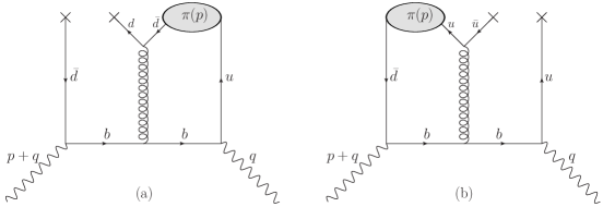
Figure 1: Diagrams representing the factorizable twist-5 and twist-6 contributions to the correlation function (15).

They are formed only by the gluon emitted from the virtual $b$-quark. Gluons emitted from the light $\bar{d}$ and $u$ quarks and converted to the quark-antiquark pair represent a genuine long-distance effect which is by default included in the DA’s. Such an implicit separation of long- and short-distance effects takes place also in the diagrams with three-particle quark-antiquark-gluon DA’s of twist 3,4.

After factorization the further calculation is straightforward albeit lengthy. The final result of the OPE for the correlation function reads:

$$F^{\rm(OPE)}_{\rm tw5,6}(q^{2},(p+q)^{2})=\alpha_{s}\langle\bar{q}q\rangle\frac{C_{F}}{N_{c}}\pi m_{b}f_{\pi}\int\limits_{0}^{1}du\int\limits_{0}^{1}dv$$

$$\times \Biggl{\{}\varphi(v)\Biggl{[}\frac{1}{[m_{b}^{2}-(q+uvp)^{2}]^{2}}+\frac{2(1-2u\bar{u})}{[m_{b}^{2}-(q+(u+v-uv)p)^{2}]^{2}}$$

$$+ \frac{4u\bar{u}\,q^{2}}{[m_{b}^{2}-(q+uvp)^{2}]^{3}}+\frac{4u\bar{u}\,m_{b}^{2}}{[m_{b}^{2}-(q+(u+v-uv)p)^{2}]^{3}}\Biggr{]}$$

$$- 4\mu_{\pi}m_{b}\,\varphi_{p}(v)\Biggl{[}\frac{u^{2}\bar{u}v}{[m_{b}^{2}-(q+uvp)^{2}]^{3}}+\frac{u\bar{u}(uv-u-v)}{[m_{b}^{2}-(q+(u+v-uv)p)^{2}]^{3}}\Biggr{]}$$

$$+ 2\mu_{\pi}m_{b}\,\varphi_{\sigma}(v)\Biggl{[}\frac{u^{2}\bar{u}(m_{b}^{2}+q^{2})}{[m_{b}^{2}-(q+uvp)^{2}]^{4}}+\frac{u\bar{u}^{2}(m_{b}^{2}+q^{2})}{[m_{b}^{2}-(q+(u+v-uv)p)^{2}]^{4}}\Biggr{]}\Biggr{\}},$$

where the contributions of factorizable twist-5 and twist-6 terms are separated. Note, that in the above the masses of the pion and light quarks are neglected, $m_{\pi}=0$ and $m_{u,d}=0$, everywhere except in the parameter $\mu_{\pi}=m_{\pi}^{2}/(m_{u}+m_{d})$.

In order to estimate the corresponding correction to the vector $B\to\pi$ form factor one follows the standard procedure of the LCSR derivation. First of all, one needs to perform the change of the integration variables in (3) in order to present the OPE result for the invariant amplitude $F(q^{2},(p+q)^{2})$ as a quasi-dispersion integral in the variable $(p+q)^{2}$. One obtains:

$$F^{\rm(OPE)}_{\rm tw5,6}(q^{2},(p+q)^{2})=\alpha_{s}\langle\bar{q}q\rangle\frac{C_{F}}{N_{c}}\pi m_{b}f_{\pi}\int\limits_{m_{b}^{2}}^{\infty}ds\sum_{n=2,3,4}\frac{g_{n}(q^{2},s)}{(s-(p+q)^{2})^{n}},$$ (21)

where the details of derivation and the explicit expressions of functions $g_{n}(q^{2},s)$ are given in Appendix.

To access the vector $B\to\pi$ form factor, one writes down the hadronic dispersion relation for the invariant amplitude $F(q^{2},(p+q)^{2})$ in the channel of the $\bar{b}\gamma_{5}d$ current with the four-momentum squared $(p+q)^{2}$. Inserting a full set of the hadronic states with quantum numbers of $B$-meson between the currents in (15) one isolates the ground state $B$-meson contribution in the dispersion integral. To this end, we need to define the hadronic matrix elements:

$$im_{b}\langle B|\bar{b}\gamma_{5}d|0\rangle=m_{B}^{2}f_{B},$$ (22)

$$\langle\pi(p)|\bar{q}\gamma^{\mu}b|B(p+q)\rangle=f^{+}_{B\pi}(q^{2})\left[2p^{\mu}+\left(1-\frac{m_{B}^{2}-m_{\pi}^{2}}{q^{2}}\right)q^{\mu}\right]+f^{0}_{B\pi}(q^{2})\,\frac{m_{B}^{2}-m_{\pi}^{2}}{q^{2}}\,q^{\mu},$$ (23)

where $f_{B}$ is the $B$-meson decay constant and $f^{+}_{B\pi}(q^{2})$ and $f^{0}_{B\pi}(q^{2})$ are the standard $B\to\pi$ vector and scalar form factors. One presents then the amplitude $F(q^{2},(p+q)^{2})$ as follows:

$$F(q^{2},(p+q)^{2})=\frac{2f_{B\pi}^{+}(q^{2})m_{B}^{2}f_{B}}{m_{B}^{2}-(p+q)^{2}}+\int\limits_{s_{0}^{B}}^{\infty}ds\frac{\rho^{h}(q^{2},s)}{s-(p+q)^{2}}.$$ (24)

In the above, the contribution of the excited states and continuum of hadrons with the same quantum numbers as $B$-meson is presented in the form of the integral over the spectral density $\rho^{h}(q^{2},s)$. Its contribution can be related with the OPE result by means of the quark-hadron duality

$$\rho^{h}(q^{2},s)=\frac{1}{\pi}{\rm Im}F^{\rm(OPE)}(q^{2},s)\,\Theta(s-s_{0}^{B}),$$ (25)

introducing the effective continuum threshold $s_{0}^{B}$. The imaginary part of the invariant amplitude ${\rm Im}F^{\rm(OPE)}(q^{2},(p+q)^{2})$ in the variable $(p+q)^{2}$ is easily extracted from (21). In order to suppress the contribution of the excited states one applies the Borel transformation, replacing the variable $(p+q)^{2}$ by the Borel parameter $M^{2}$. Finally, after substraction of the continuum contribution the corresponding twist-5 and twist-6 corrections for the vector $B\to\pi$ form factor can be presented in the following compact form:

$$\left[f_{B\pi}^{+}(q^{2})\right]_{\rm tw5,6}=\left(\frac{e^{m_{B}^{2}/M^{2}}}{2m_{B}^{2}f_{B}}\right)\alpha_{s}\langle\bar{q}q\rangle\frac{C_{F}}{N_{c}}\pi m_{b}f_{\pi}\int\limits_{m_{b}^{2}}^{\infty}\!ds\!\sum_{n=2,3,4}\!\!\rho_{n}(q^{2},s;s_{0}^{B},M^{2})$$ (26)

with the auxiliary functions $\rho_{n}(q^{2},s;s_{0}^{B},M^{2})$ taking the form

$$\rho_{n}(q^{2},s;s_{0}^{B},M^{2})=\frac{(-1)^{n-1}}{(n-1)!}\,g_{n}(q^{2},s)\frac{d^{n-1}}{ds^{n-1}}\left[\theta(s_{0}^{B}-s)e^{-s/M^{2}}\right],$$ (27)

where the derivatives in $s$ emerge due to the higher power of the denominator in (21), yielding the surface terms in the LCSR at $s=s_{0}^{B}$.

4 Numerical analysis

	$q^{2}=0$	$q^{2}=10$ GeV2
$f_{B\pi}^{+}(q^{2})$	0.301	0.562
Tw2 LO	$47.5\%$	$48.2\%$
Tw2 NLO	$6.9\%$	$5.9\%$
Tw3 LO	$50.0\%$	$54.2\%$
Tw3 NLO	$-4.6\%$	$-7.5\%$
Tw4 LO	$0.2\%$	$-0.8\%$
Tw5 LO, fact	$-0.034\%$	$-0.042\%$
Tw6 LO, fact	$-0.004\%$	$-0.011\%$

Table 1: The value of the $B\to\pi$ form factor at two typical values $q^{2}=0$ and $q^{2}=10$ GeV² and the partial contributions to the LCSR.

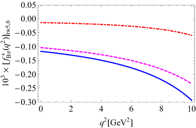
Figure 2: The factorizable twist-5 and twist-6 corrections to the vector $B\to\pi$ form factor. The dot-dashed (red) curve is the twist 6. The dashed (magenta) one is the twist 5 and the solid (blue) curve is the sum of the two.

In order to estimate the numerical impact of the factorizable twist-5 and twist-6 terms on the vector $B\to\pi$ form factor we need to specify the input used in the LCSR. First of all, the values of the $B$-mesons mass $m_{B^{0}}=5.27931\,{\rm GeV}$ and the pion decay constant $f_{\pi}=130.4\,{\rm MeV}$ are taken from [14]. The mass of $b$-quark is used in $\overline{MS}$-scheme and we adopt the interval $\overline{m}_{b}(\overline{m}_{b})=4.18\pm 0.03$ GeV [14]. The value of the quark condensate density $\langle\bar{q}q\rangle(2\,{\rm GeV})=-(277^{+12}_{-10}\,{\rm MeV})^{3}$ is taken from [15]. The normalization parameter of the twist-3 DAs $\mu_{\pi}$ is determined by means of ChPT relations and we use $\mu_{\pi}(2\,{\rm GeV})=2.50\,{\rm GeV}$ following [16]. For the renormalization scale we use the value $\mu=3\,{\rm GeV}$. The $B$-meson decay constant can be extracted from the QCD sum rules and we apply the value $f_{B}=202\,{\rm MeV}$ corresponding to the NLO accuracy of the corresponding sum rules [15]. Furthermore, the Borel parameter $M^{2}$ and the continuum threshold $s_{0}^{B}$ are taken at their typical values $M^{2}=16\,{\rm GeV}^{2}$ and $s_{0}^{B}=37.2\,{\rm GeV}^{2}$ used as central values in the most recent paper [17].

Concerning the choice of the twist-2 and twist-3 pion DAs, we restrict ourselves by the asymptotic form $\varphi(v)=6v\bar{v}$, $\varphi_{p}(v)=1$ and $\varphi_{\sigma}(v)=6v\bar{v}$, sufficient for our accuracy having in mind that the nonasymptotic corrections to these DA’s are relatively small. Implementing the explicit forms for the DA’s allows to perform an integration over $u$ in (34) - (36) and to determine the auxiliary functions $g_{n}(q^{2},s)$ entering the LCSR for the vector $B\to\pi$ form factor (26).

The numerical results for $f_{B\pi}^{+}(q^{2})$ corresponding to the above described input are presented in Fig. 2, where the $q^{2}$-dependence of the factorizable twist-5 and twist-6 corrections is plotted. Note that the corrections grow al large $q^{2}$ as it should be, reflecting the growth of the higher twists effects in the region of low recoil, where OPE starts to diverge. In Tab. 1 we present separate contributions to the LCSR for the vector $B\to\pi$ form factor at two typical values $q^{2}=0$ and $q^{2}=10$ GeV² in order to demonstrate the magnitude of the factorizable higher twist corrections to the vector $B\to\pi$ form factor. We found that in the whole domain of $q^{2}$ of the LCSR applicability the relative contributions of the higher twist effects do not exceed $0.05\%$ revealing their strong suppression. The obtained result justifies a standard truncation of the OPE in LCSR up to the twist-4 terms. It is important to note that one of the sources of such suppression is a largeness of the $b$-quark mass. We also extended the analysis for the LCSRs for other, $B\to K$ and $B_{s}\to K$ transition vector form factors. We found that in all these cases, the factorizable higher twist effects are also significantly suppressed. The corresponding corrections could have more sizeable effects in the case of $D\to\pi$ and $D\to K$ from factor due to a smaller value of the $c$-quark mass. We plan to perform such analysis in the future.

5 Conclusion

In this paper we estimate the higher twist effects in the LCSR for the $B\to\pi$ vector form factor in the framework of the factorization approximation. To this end, the light-cone expansion of the massive quark propagator including the higher derivatives of the gluon-field strength is derived. The corresponding expression is in agreement with the leading order expansion of the massive propagator [4] and in the massless quark limit reproduces the propagator obtained in [10]. Our result has a more general relevance since it can be used in any other application of LCSR where one needs the LC-expansion of the massive quark propagator. We derive the analytical expressions for the factorizable twist-5 and twist-6 contributions to the LCSR for the vector $B\to\pi$ form factor. The relevant numerical analysis reveals that these effects are extremely suppressed. This justifies the conventional truncation of the operator product expansion in the light-cone sum rules up to twist-4 terms adopted in the previous LCSR analyses.

Appendix

In order to present the OPE result for the correlation function in the form of dispersion integral we need to perform some transformations. The integrals

$$I_{n}=\int\limits_{0}^{1}\!\int\limits_{0}^{1}dv\,du\,\frac{f_{n}(q^{2},u,v)}{[m_{b}^{2}-(q+uvp)^{2}]^{n}},\quad n=2,3,4,$$ (28)

result from the diagram (a) of Fig. 1, and

$$J_{n}=\int\limits_{0}^{1}\!\int\limits_{0}^{1}dv\,du\,\frac{\bar{f}_{n}(q^{2},u,v)}{[m_{b}^{2}-(q+(u+v-uv)p)^{2}]^{n}},\quad n=2,3,4,$$ (29)

from diagram (b). The functions $f_{n}(q^{2},u,v)$ and $\bar{f}_{n}(q^{2},u,v)$ can be easily read off eq. (3). Our task is to present both $I_{n}$ and $J_{n}$ in the form of dispersion integral. To this end, in the integrals $I_{n}$ of the first type we replace the variable $v$ by $\alpha=uv$, and change then the integration order

$$\int\limits_{0}^{1}du\int\limits_{0}^{u}d\alpha\,(\ldots)=\int\limits_{0}^{1}d\alpha\int\limits_{\alpha}^{1}du\,(\ldots).$$

Afterwards, we introduce a new variable $s$ as follows

$$\alpha=\frac{m_{b}^{2}-q^{2}}{s-q^{2}}\equiv u_{1}(s,q^{2}).$$ (30)

Finally, the integrals $I_{n}$ transform to

$$I_{n}=\int\limits_{m_{b}^{2}}^{\infty}ds\!\!\!\int\limits_{u_{1}(s,q^{2})}^{1}\!\!\!\frac{du}{u}\frac{(s-q^{2})^{n-2}}{(m_{b}^{2}-q^{2})^{n-1}}\frac{f_{n}\left(q^{2},u,\displaystyle\frac{m_{b}^{2}-q^{2}}{u(s-q^{2})}\right)}{(s-(p+q)^{2})^{n}}.$$ (31)

For the integrals of the second type $J_{n}$ we perform the replacements $u\to 1-u=\bar{u}$ and $v\to 1-v=\bar{v}$. The next steps are similar to the previous case and the integrals $J_{n}$ finally transform to

$$J_{n}=\int\limits_{m_{b}^{2}}^{\infty}ds\!\!\!\int\limits_{u_{2}(s,q^{2})}^{1}\!\!\!\frac{d\bar{u}}{\bar{u}}\frac{(s-q^{2})^{n-2}}{(m_{b}^{2}-q^{2})^{n-1}}\frac{\bar{f}_{n}\left(q^{2},\bar{u},\displaystyle\frac{s-m_{b}^{2}}{\bar{u}(s-q^{2})}\right)}{(s-(p+q)^{2})^{n}},$$ (32)

with $u_{2}(s,q^{2})$ defined as:

$$u_{2}(s,q^{2})=\frac{s-m_{b}^{2}}{s-q^{2}}.$$ (33)

Note, that in the above integrals the dependence on the variable $(p+q)^{2}$ is reduced to the denominator in the form $(s-(p+q)^{2})^{n}$. This significantly simplifies the derivation of the LCSR for the correlation function. With help of (31) and (32), the OPE result for the correlation function transforms to the quasi-dispersion form (21) with the functions $g_{n}(q^{2},s)$ listed below:

$$g_{2}(q^{2},s) = \frac{1}{m_{b}^{2}-q^{2}}\int\limits_{u_{1}}^{1}\frac{du}{u}\varphi(u_{1}/u)+\frac{2}{m_{b}^{2}-q^{2}}\int\limits_{u_{2}}^{1}\frac{du}{u}(1-2u\bar{u})\varphi(u_{2}/u),$$ (34)

$$g_{3}(q^{2},s) = \frac{4q^{2}(s-q^{2})}{\left(m_{b}^{2}-q^{2}\right)^{2}}\int\limits_{u_{1}}^{1}du\,\bar{u}\,\varphi(u_{1}/u)-\frac{4\mu_{\pi}m_{b}}{m_{b}^{2}-q^{2}}\int\limits_{u_{1}}^{1}du\,\bar{u}\,\varphi_{p}(u_{1}/u)$$ (35)

$$+ \frac{4m_{b}^{2}(s-q^{2})}{\left(m_{b}^{2}-q^{2}\right)^{2}}\int\limits_{u_{2}}^{1}du\,\bar{u}\,\varphi(u_{2}/u)+\frac{4\mu_{\pi}m_{b}}{m_{b}^{2}-q^{2}}\int\limits_{u_{2}}^{1}du\,\bar{u}\,\varphi_{p}(u_{2}/u),$$

$$g_{4}(q^{2},s) = 2\mu_{\pi}m_{b}\frac{\left(s-q^{2}\right)^{2}\left(m_{b}^{2}+q^{2}\right)}{\left(m_{b}^{2}-q^{2}\right)^{3}}\int\limits_{u_{1}}^{1}duu\bar{u}\,\varphi_{\sigma}(u_{1}/u)$$ (36)

$$+ 2\mu_{\pi}m_{b}\frac{\left(s-q^{2}\right)^{2}\left(m_{b}^{2}+q^{2}\right)}{\left(m_{b}^{2}-q^{2}\right)^{3}}\int\limits_{u_{2}}^{1}duu\bar{u}\,\varphi_{\sigma}(u_{2}/u),$$

where $u_{1,2}=u_{1,2}(s,q^{2})$ are already defined in (30) and (33). Inserting the explicit expressions for the pion LCDA’s $\varphi(v),\varphi_{p}(v)$ and $\varphi_{\sigma}(v)$ allows to perform an integration over variable $u$ in (34), (35) and (36).

References

• [1] I.I. Balitsky, V.M. Braun and A.V. Kolesnichenko, Sov. J. Nucl. Phys.  44 (1986) 1028 [Yad. Fiz.  44 (1986) 1582].
• [2] V.L. Chernyak and I.R. Zhitnitsky, Nucl. Phys. B 345 (1990) 137.
• [3] V.M. Belyaev, A. Khodjamirian and R. Ruckl, Z. Phys. C 60 (1993) 349, hep-ph/9305348.
• [4] V.M. Belyaev, V.M. Braun, A. Khodjamirian and R. Ruckl, Phys. Rev. D 51 (1995) 6177, hep-ph/9410280.
• [5] G. Duplancic, A. Khodjamirian, T. Mannel, B. Melic and N. Offen, JHEP 0804 (2008) 014, arXiv:0801.1796 [hep-ph].
• [6] A. Khodjamirian, R. Ruckl, S. Weinzierl and O.I. Yakovlev, Phys. Lett. B 410 (1997) 275, hep-ph/9706303.
• [7] E. Bagan, P. Ball and V.M. Braun, Phys. Lett. B 417 (1998) 154, hep-ph/9709243.
• [8] P. Ball and R. Zwicky, JHEP 0110 (2001) 019, hep-ph/0110115.
• [9] A. Bharucha, JHEP 1205 (2012) 092, arXiv:1203.1359 [hep-ph].
• [10] I.I. Balitsky and V.M. Braun, Nucl. Phys. B 311 (1989) 541.
• [11] V.M. Braun, A. Khodjamirian and M. Maul, Phys. Rev. D 61 (2000) 073004, hep-ph/9907495.
• [12] S.S. Agaev, V.M. Braun, N. Offen and F.A. Porkert, Phys. Rev. D 83 (2011) 054020, arXiv:1012.4671 [hep-ph].
• [13] P. Colangelo and A. Khodjamirian, In *Shifman, M. (ed.): At the frontier of particle physics, vol. 3* 1495-1576, hep-ph/0010175.
• [14] C. Patrignani et al. [Particle Data Group], Chin. Phys. C 40 (2016), 100001.
• [15] P. Gelhausen, A. Khodjamirian, A.A. Pivovarov and D. Rosenthal, Phys. Rev. D 88 (2013) 014015, Erratum: [Phys. Rev. D 89 (2014) 099901], Erratum: [Phys. Rev. D 91 (2015) 099901], arXiv:1305.5432 [hep-ph].
• [16] A. Khodjamirian, C. Klein, T. Mannel and N. Offen, Phys. Rev. D 80 (2009) 114005, arXiv:0907.2842 [hep-ph].
• [17] A. Khodjamirian and A.V. Rusov, arXiv:1703.04765 [hep-ph].