Measurements of $ep\to e^{\prime}\pi^{+}\pi^{-}p^{\prime}$ Cross Sections with CLAS at 1.40 GeV $<$ $W$ $<$ 2.0 GeV and 2.0 GeV² $<Q^{2}<$ 5.0 GeV²

Abstract

This paper reports new exclusive cross sections for $ep\to e^{\prime}\pi^{+}\pi^{-}p^{\prime}$ using the CLAS detector at Jefferson Laboratory. These results are presented for the first time at photon virtualities 2.0 GeV² $<Q^{2}<5.0$ GeV² in the center-of-mass energy range 1.4 GeV $<W<$ 2.0 GeV, which covers a large part of the nucleon resonance region. Using a model developed for the phenomenological analysis of electroproduction data, we see strong indications that the relative contributions from the resonant cross sections at $W<1.74$ GeV increase with $Q^{2}$. These data considerably extend the kinematic reach of previous measurements. Exclusive $ep\to e^{\prime}\pi^{+}\pi^{-}p^{\prime}$ cross section measurements are of particular importance for the extraction of resonance electrocouplings in the mass range above 1.6 GeV.

I Introduction

An extensive research program aimed at the exploration of the structure of excited nucleon states is in progress at Jefferson Lab, employing exclusive meson electroproduction off protons in the nucleon resonance ($N^{*}$) region. This represents an important direction in a broad effort to analyze data from the CLAS detector Aznauryan and Burkert (2012); Aznauryan et al. (2013, ).

Many nucleon states in the mass range above 1.6 GeV are known to couple strongly to $\pi\pi N$. Therefore, studies of exclusive $\pi^{+}\pi^{-}p$ electroproduction are a major source of information on the internal structure of these states. Studies of exclusive $\pi^{+}\pi^{-}p$ electroproduction are of particular importance for the extraction of the $N^{*}$ electrocoupling amplitudes off protons for all prominent resonances in the mass range up to 2.0 GeV and at photon virtualities $Q^{2}<5.0$ GeV².

The $\gamma_{v}pN^{*}$ electrocouplings are the primary source of information on many facets of non-perturbative strong interactions, particularly in the generation of the excited proton states from quarks and gluons. Analyses of the $\gamma_{v}pN^{*}$ electrocouplings extracted from CLAS have already revealed distinctive differences in the electrocouplings of states with different underlying quark structures, e.g. orbital versus radial quark excitations Aznauryan and Burkert (2012); Aznauryan et al. (2013, ).

Furthermore, the structure of excited nucleons represents a complex interplay between the inner core of three dressed quarks and the external meson-baryon cloud Aznauryan and Burkert (2012); Mokeev et al. (2016a); Aznauryan and Burkert (2015); Suzuki et al. (2010), with their relative contributions evolving with photon virtuality. Therefore, measurements of $\gamma_{v}pN^{*}$ electrocouplings allow for a detailed charting of the spatial structure of nucleon resonances in terms of their quark cores and higher Fock states. Studies of many prominent resonances are needed in order to explore the full complexity of non-perturbative strong interactions in the generation of different excited states. It is through such information that models built on ingredients from QCD are to be confronted, and lead to new insights into the strong interaction dynamics, as well as developments of new theoretical approaches to solve QCD in these cases.

The unique interaction of experiment and theory was recently demonstrated on the quark distribution amplitudes (DAs) for the $N(1535)1/2^{-}$ resonance (a chiral partner of the nucleon ground state). These DAs have become available from Lattice QCD Braun et al. (2014), constrained by the CLAS results on the transition $N\to N(1535)1/2^{-}$ form factor Aznauryan et al. (2009), by employing DAs and the Light Cone Sum Rule (LCSR) approach Anikin et al. (2015). The comparison of quark DAs in the nucleon ground state and in the $N(1535)1/2^{-}$ resonance demonstrates a pronounced difference, elucidating the manifestation of Dynamical Chiral Symmetry Breaking (DCSB) in the structure of the ground and excited nucleon states.

Recent advances in Dyson-Schwinger Equations (DSEs) now make it possible to describe the elastic nucleon and the transition form factors for $N\to\Delta(1232)3/2^{+}$ and $N\to N(1440)1/2^{+}$ starting from the QCD Lagrangian Segovia and others (2014); Segovia et al. (2015). Currently, DSEs relate the $\gamma_{v}pN^{*}$ electrocouplings to the quark mass function at distance scales of $Q^{2}>2$ GeV², where the quark core is the biggest contributor to the $N^{*}$ structure. This success demonstrates the relevance of dressed constituent quarks inferred within the DSEs Cloët and Roberts (2014) as effective degrees of freedom in the structure of the ground and excited nucleon states, and emphasizes the need for data on the $Q^{2}$ dependence of the $\gamma_{v}pN^{*}$ electrocouplings to provide access to the momentum dependence of the dressed quark mass. This can provide new insight into two of the still open problems of the Standard Model, namely the nature of hadron mass and the emergence of quark-gluon confinement from QCD Roberts (2016, 2016); Cloët and Roberts (2014).

The CLAS Collaboration has provided much of the world data on meson electroproduction in the resonance excitation region. Nucleon resonance electrocouplings have been obtained from the exclusive channels: $\pi^{+}n$ and $\pi^{0}p$ at $Q^{2}<5.0$ GeV² in the mass range up to 1.7 GeV, $\eta p$ at $Q^{2}<4.0$ GeV² in the mass range up to 1.6 GeV, and $\pi^{+}\pi^{-}p$ at $Q^{2}<1.5$ GeV² in the mass range up to 1.8 GeV Mokeev et al. (2016a); Aznauryan and Burkert (2012); Aznauryan et al. (2009); Park et al. (2015); Mokeev et al. (2012); Mokeev and Aznauryan (2014); Mokeev et al. (2016b); Mokeev (2016). The studies of the $N(1440)1/2^{+}$ and $N(1520)3/2^{-}$ resonances with the CLAS detector Mokeev et al. (2016a); Aznauryan et al. (2009); Mokeev et al. (2012) have provided most of the information available worldwide on these electrocouplings in the range 0.25 GeV${}^{2}<Q^{2}<5.0$ GeV². The $N(1440)1/2^{+}$ and $N(1520)3/2^{-}$ states, together with the $\Delta(1232)3/2^{+}$ and $N(1535)1/2^{-}$ resonances, are the best understood excited nucleon states to date Aznauryan and Burkert (2012). Furthermore, results on the $\gamma_{v}pN^{*}$ electrocouplings for the high-lying $N(1675)5/2^{-}$, $N(1680)5/2^{+}$, and $N(1710)1/2^{+}$ resonances were determined from the CLAS $\pi^{+}n$ data at 1.5 GeV${}^{2}<Q^{2}<4.5$ GeV² Park et al. (2015).

Many excited nucleon states with masses above 1.6 GeV decay preferentially to the $\pi\pi N$ final states, making exclusive $\pi^{+}\pi^{-}p$ electroproduction off protons a major source of information on these electrocouplings. First accurate results on the electrocouplings of the $\Delta(1620)1/2^{-}$, which couples strongly to $\pi\pi N$, have been published from the analysis of CLAS data on $\pi^{+}\pi^{-}p$ electroproduction off protons Mokeev et al. (2016a). Preliminary results on electrocouplings of two other resonances, the $\Delta(1700)3/2^{-}$ and the $N(1720)3/2^{+}$, show dominance of $\pi\pi N$ decays and were obtained from the $\pi^{+}\pi^{-}p$ data Mokeev and Aznauryan (2014). Previous studies of these resonances in the $\pi N$ final states suffered from large uncertainties due to small branching fractions for decays to $\pi N$.

The combined analysis of the $\pi^{+}\pi^{-}p$ photo- and electroproduction data Ripani et al. (2003) revealed preliminary evidence for the existence of a $N^{\prime}(1720)3/2^{+}$ state. Its spin-parity, mass, total and partial hadronic decay widths, along with the $Q^{2}$ evolution of its $\gamma_{v}pN^{*}$ electrocouplings, have been obtained from a fit to the CLAS data Mokeev et al. (2016b). This is the only new candidate state for which information on $\gamma_{v}pN^{*}$ electrocouplings has become available, offering access to its internal structure. A successful description of the photo- and electroproduction data with $Q^{2}$ independent mass and hadronic decay widths offers nearly model-independent evidence for the existence of this state. Future studies of exclusive $\pi^{+}\pi^{-}p$ electroproduction off protons at $W>1.7$ GeV will also open up the possibility to verify new baryon states observed in a global multi-channel analysis of exclusive photoproduction data by the Bonn-Gatchina group Anisovich et al. (2012).

The resonance electrocouplings from exclusive $\pi^{+}\pi^{-}p$ electroproduction off protons have been extracted in the range of $W<2.0$ GeV and $Q^{2}<1.5$ GeV² Ripani et al. (2003); Fedotov et al. (2009). An extension of the measured $\pi^{+}\pi^{-}p$ electroproduction cross sections towards higher photon virtualities is critical for the extraction of resonance electrocouplings at the distance scale where the transition to the dominance of dressed quark degrees of freedom in the $N^{*}$ structure is expected Aznauryan and Burkert (2012); Aznauryan et al. (2013). These data will provide input for reaction models aimed at determining $\gamma_{v}pN^{*}$ electrocouplings for the $N^{*}$ resonances in the mass range above 1.6 GeV Mokeev et al. (2009, 2012, 2016a). These data will also provide necessary input for global multi-channel analyses of the exclusive meson photo-, electro-, and hadroproduction channels Anisovich et al. (2012, 2014); Suzuki et al. (2010); Kamano et al. (2013, 2016).

In this paper we present cross sections for $\pi^{+}\pi^{-}p$ electroproduction off protons at center of mass energies $W$ from 1.4 GeV to 2.0 GeV and at $Q^{2}$ from 2.0 GeV² to 5.0 GeV² in terms of nine independent 1-fold differential and fully integrated $\pi^{+}\pi^{-}p$ cross sections. As in our previous studies Ripani et al. (2003); Fedotov et al. (2009), these are obtained by integration of the 5-fold differential cross section over different sets of four kinematic variables. The combined analysis of all nine 1-fold differential cross sections gives access to correlations in the 5-fold differential cross sections from the correlations seen in the nine 1-fold differential cross sections, as they all represent different integrals of the same 5-fold differential cross sections.

II Experimental Description

The data were collected using the CLAS detector Mecking et al. (2003) with an electron beam of 5.754 GeV incident on a liquid-hydrogen target. The beam current averaged about 7 nA and was produced by the Continuous Electron Beam Accelerator Facility (CEBAF) at the Thomas Jefferson National Accelerator Laboratory (TJNAF). The liquid-hydrogen target had a length of 5.0 cm and was placed 4.0 cm upstream of the center of the CLAS detector. The torus coils of the CLAS detector were operated at 3375 A and an additional mini-torus close to the target was run at 6000 A to remove low-energy background electrons. The CLAS spectrometer consisted of a series of detectors in each of its six azimuthal sectors, including three sets of wire drift-chambers (DC) for tracking scattered charged particles, Cerenkov counters (CC) to distinguish electrons and pions, sampling electromagnetic calorimeters (EC) for electron and neutral particle identification, and a set of time-of-flight scintillation counters (SC) to record the flight time of charged particles. For this experiment, the data acquisition triggered on a coincidence between signals in the CC and EC, as explained below. This configuration of the experiment was called the CLAS e1-6 run to distinguish it from other data sets.

II.1 Selection of Electrons

The particle tracks were determined from the DC coordinates and extrapolated back to the target position. A coordinate system was defined with the $z$-axis along the beam direction. A histogram of a sampling of electron tracks extrapolated to their point of closest approach to the $z$-axis is shown in Fig. 1 for one of the six sectors of the CLAS detector. Plots for the other sectors are very similar. A small correction was made for the positioning of the DC in each sector to align the target position. Event selection required a good event to come from the target region.

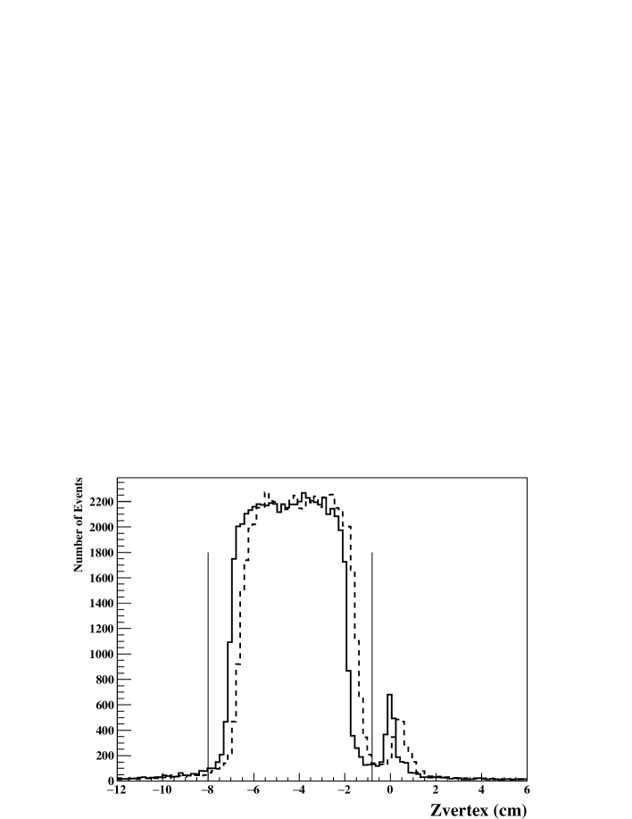
Figure 1: Vertex reconstruction projected onto the beam axis for Sector 2 of CLAS, before (dashed) and after (black) applying corrections to align the sectors of CLAS. The vertical lines show the region of the vertex event selection. The small peak at zero originates from an aluminum window 2 cm downstream of the target cell.

A scattered electron produced an electromagnetic shower of particles in the EC, and the characteristics of this shower were different for pions and electrons. However, the electromagnetic shower was not fully contained at the edges of the EC, so it was necessary to place an event selection cut to remove these unwanted events near the edges. This cut on the fiducial volume is shown in Fig. 2. The edges of the fiducial regions were chosen based on studies of the EC resolution and the comparison with known cross sections for elastic $e-p$ scattering.

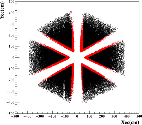
Figure 2: (Color Online) The position of electron events in the EC for the six sectors of CLAS for all events (light gray or red online) and selected events (black). The stripe seen in the lower left sector is due to inefficient phototubes on a few scintillator strips of the EC. The same inefficiencies are introduced in the simulations of the detector acceptance.

The EC has two layers, an inner layer (closer to the target) and an outer layer. See Ref. Mecking et al. (2003) for more details on the EC geometry. The two layers enabled separation of charged pions and electrons. Normally incident minimum ionizing pions typically lost 26 MeV of energy in the 15 cm of scintillating material of the inner part of the calorimeter, whereas electrons that underwent an electromagnetic shower, deposited more energy ($E_{in}$) in the inner EC layer. A data selection cut $E_{in}>60$ MeV eliminated most of the pions, as shown in Fig. 3. A further refined selection of electrons came from the correlation between total energy deposited and momentum. An additional momentum-dependent cut was placed on the ratio of the total energy in the EC and the momentum, $E_{tot}/p$. For a given momentum, the data formed a Gaussian peak for this ratio centered near 0.3. A 2.5$\sigma$ cut on this peak was applied to the data. The loss of events in the Gaussian tail was accounted for by the detector acceptance, where an equivalent cut was placed on the Monte Carlo simulation data.

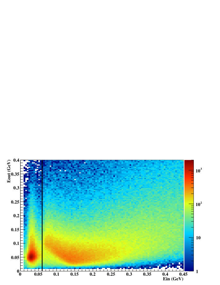
Figure 3: (Color Online) The energy deposited in the inner ($E_{in}$) and outer ($E_{out}$) layers of the EC for all particles. The line corresponds to 60 MeV, which separates the minimum ionizing pions (to the left) and electrons (to the right).

II.2 Particle Identification

Particle identification for hadrons was obtained comparing the particle velocity evaluated from the flight time (from the target to the SC) and from the momentum of the particle track (measured by the DC) for an assumed mass. When the assumed particle mass is correct, the particle’s velocity calculated from both methods agrees. Fig. 4 top and bottom show the difference between the velocity calculated from the time-of-flight and that from the momentum for pions and protons, respectively, which gives a horizontal band about zero velocity difference. Below a momentum of about 2 GeV, this method provides excellent separation between pions and protons, and reasonable separation up to 2.5 GeV.

For the e1-6 run, the current in the torus coils was set such that positively charged particles bent outward and negatively charged particles bent inward. In this data run, some regions of the CLAS detector were inefficient, due to bad sections of the DC or bad SC paddle PMTs. An example is shown in Fig. 5 for positively charged pions in Sector 3. The inefficient detector regions show up clearly in a plot of the measured track momentum $p$ versus the polar angle $\theta$ of the track. These regions were cut out of both the data and Monte Carlo simulation, providing a good match between the real and simulated detector acceptance. In addition, cuts were placed to restrict particle tracks to the fiducial volume of the detector, which eliminated inefficient regions at the edges of the CC and DC. The fiducial cuts are standard for CLAS and are described elsewhere Ripani et al. (2003).

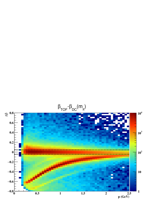
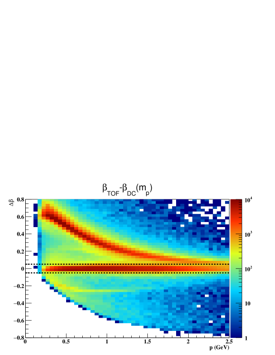
Figure 4: (Color Online) Velocity difference $\beta_{TOF}-\beta_{DC}$ for a sample of positively charged tracks versus momentum for assumed masses of a pion (top) or a proton (bottom).

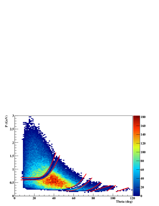
Figure 5: (Color Online) Histogram of the correlation between the momentum $p$ and the polar angle $\theta$ for tracks of positively charged pions in Sector 3 of CLAS. The inefficient regions of the detector, shown between the bands of solid lines, were removed from the analysis.

II.3 Event Selection

Events with a detected electron, proton, and positively charged pion were retained for further analysis. The reaction of interest here is $ep\to e^{\prime}\pi^{+}\pi^{-}p^{\prime}$, where the primed quantities are for the final state. The negative pion was bent toward the beamline and could bend outside of the detector acceptance. We reconstructed the mass of the $\pi^{-}$ using the missing mass technique. The missing mass squared $M_{X}^{2}$ for these $ep\to e^{\prime}p^{\prime}\pi^{+}X$ events is shown in Fig. 6, with a clean peak at the pion mass. The peak position and width compared very well with Monte Carlo (MC) simulated events. The larger number of events in the data at higher missing mass is due to radiative events, where the electron radiated a low-energy photon either before, after, or during the scattering off the proton. The loss of these events from the peak was calculated using standard methods (described later in Section II.7) and was corrected for in the final analysis. After all selections were applied, there remained 336,668 exclusive $\pi^{+}\pi^{-}p$ events. The distribution of data events for this measurement is shown in Fig. 7 as a function of the center of mass (CM) energy $W$ and the squared 4-momentum transfer to the virtual photon $Q^{2}$. The data were binned, as shown by the black lines in the plot, to get the fully integrated cross section dependence on $W$ and $Q^{2}$.

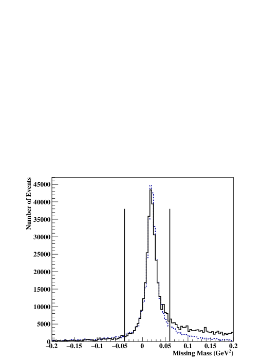
Figure 6: Square of the missing mass $M_{X}^{2}$ for $ep\to e^{\prime}\pi^{+}\pi^{-}p^{\prime}$, showing a peak at the $\pi^{-}$ mass squared. The dashed histogram is from the Monte Carlo and the solid histogram is the data. The vertical lines show the applied cut.

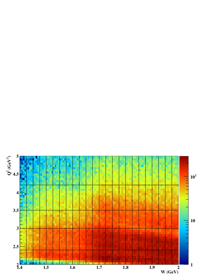
Figure 7: (Color Online) The kinematic coverage of the data, shown as a scatter-plot of events as a function of center of mass energy $W$ and squared 4-momentum transfer $Q^{2}$. Bins are shown within which the integrated and nine 1-fold differential $\pi^{+}\pi^{-}p$ cross sections were obtained.

II.4 Reaction Kinematics

The kinematics of the reaction is shown in Fig. 8. The scattered electron defines a plane, which in our coordinate system is the $x-z$ plane. The direction of the $z$-axis was chosen to align with the virtual photon momentum vector. The $y$-axis is normal to the scattering plane with its direction defined by the vector product $\vec{n}_{y}=\vec{n}_{z}\times\vec{n}_{x}$ as shown in Fig. 8. The virtual photon and the outgoing $\pi^{-}$ form another plane, labeled A in Fig. 8, with angles $\theta$ and $\phi$ as shown. We also need the $\theta$ and $\phi$ angles for the $\pi^{+}$ and the final state proton $p^{\prime}$, as described next.

Figure 8: Angular variables from the set defined by Eq. (13) for the description of the $ep\to e^{\prime}\pi^{+}\pi^{-}p^{\prime}$ reaction in the CM frame of the final state hadrons. Panel (a) shows the $\pi^{-}$ spherical angles $\theta_{\pi^{-}}$ and $\varphi_{\pi^{-}}$. Plane A is defined by the 3-momenta of the initial state proton and the final state $\pi^{-}$. Plane C represents the electron scattering plane. Panel (b) shows the angle $\alpha_{[\pi^{-}p][\pi^{+}p^{\prime}]}$ between the two defined hadronic planes A and B. Plane B is defined by the 3-momenta of the final state $\pi^{+}$ and $p^{\prime}$. The unit vectors $\vec{\gamma}$ and $\vec{\beta}$ are normal to the $\pi^{-}$ 3-momentum in the planes A and B, respectively.

Another plane is defined by the outgoing particles $\pi^{+}$ and $p^{\prime}$, labeled B in Fig. 8, which intersects with plane A. Note that in the CM frame, the 3-momenta of all three final state hadrons are located in the common plane B. The angle between the A and B planes is given by $\alpha_{[\pi^{-}p][\pi^{+}p^{\prime}]}$ as shown in Fig. 8. In order to calculate this angle, the vectors $\vec{\beta}$, $\vec{\gamma}$, and $\vec{\delta}$ are defined as shown in Fig. 8 and evaluated as given in Fedotov et al. (2009).

The 3-body final state is unambiguously determined by 5 kinematic variables. Indeed, three final state particles could be described by $4\times 3=12$ components of their 4-momenta. As each of these particles was on-shell, this provided three restrictions $E_{i}^{2}-P_{i}^{2}=m_{i}^{2}$ $(i=1,2,3)$. Energy-momentum conservation imposed four additional constraints for the final state particles, so that there were five remaining kinematic variables that unambiguously determine the 3-body final state kinematics. In the electron scattering process $ep\to e\pi^{+}\pi^{-}p^{\prime}$, we also have the variables $W$ and $Q^{2}$ that fully define the initial state kinematics. So the electron scattering cross sections for double charged pion production should be 7-fold differential: 5 variables for the final state hadrons, plus $W$ and $Q^{2}$ determined by the electron scattering kinematics. Such 7-fold differential cross sections may be written as $\frac{d^{7}\sigma}{dWdQ^{2}d^{5}\tau_{i}}$, where $d^{5}\tau$ is the 5-fold phase space for the final state hadron kinematics. Three sets of five kinematic variables were used with the spherical angles $\theta_{i}$ and $\varphi_{i}$ of the final state particle $\pi^{-}$, $\pi^{+}$, or $p^{\prime}$, with the differentials labeled as $d^{5}\tau_{i}$, $i$= $\pi^{-}$, $\pi^{+}$, or $p^{\prime}$, respectively. In addition to the spherical angles defined above, two other variables include the two invariant masses $M_{i,j}$ of the final state hadrons $i$ and $j$. The final variable represents the angle between the two planes A and B shown in Fig. 8, where plane A is formed by the three momenta of the initial state proton and the $i$-th final hadron, while plane B is formed by the pair of the three momenta of other two final state hadrons.

The five variables for $i=\pi^{-}$ $(M_{\pi^{+}\pi^{-}},M_{\pi^{+}p^{\prime}}$, $\theta_{\pi^{-}}$, $\varphi_{\pi^{-}}$, and $\alpha_{[\pi^{-}p][\pi^{+}p^{\prime}]})$ were calculated from the 3-momenta of the final state particles $\vec{P}_{\pi^{-}}$, $\vec{P}_{\pi^{+}}$, and $\vec{P}_{p^{\prime}}$. Two other sets with respect to the $\pi^{+}$ and $p^{\prime}$ were obtained by cyclic permutation of the aforementioned variables of the first set. All 3-momenta used from hereon, if not specified otherwise, were defined in the CM frame.

The $M_{\pi^{+}\pi^{-}}$ and $M_{\pi^{+}p^{\prime}}$ invariant masses were related to the 4-momenta of the final state particles as

$$M_{\pi^{+}\pi^{-}}=\sqrt{(P_{\pi^{+}}+P_{\pi^{-}})^{2}}~{}~{}\textrm{and}$$

$$M_{\pi^{+}p^{\prime}}=\sqrt{(P_{\pi^{+}}+P_{p^{\prime}})^{2}}\textrm{ ,}$$ (1)

where $P_{i}$ represents the final state particle 4-momentum.

The angle $\theta_{\pi^{-}}$ between the 3-momentum of the initial state photon and the final state $\pi^{-}$ in the CM frame was calculated as

$$\theta_{\pi^{-}}=\cos^{-1}\left(\frac{(\vec{P}_{\pi^{-}}\cdot\vec{P}_{\gamma})}{|\vec{P}_{\pi^{-}}||\vec{P}_{\gamma}|}\right).$$ (2)

The $\varphi_{\pi^{-}}$ angle was defined in a case-dependent manner by

$$\varphi_{\pi^{-}}=\tan^{-1}\left(\frac{P_{y\pi^{-}}}{P_{x\pi^{-}}}\right): P_{x\pi^{-}}>0,P_{y\pi^{-}}>0;$$ (3)

$$\varphi_{\pi^{-}}=\tan^{-1}\left(\frac{P_{y\pi^{-}}}{P_{x\pi^{-}}}\right)+2\pi: P_{x\pi^{-}}>0,P_{y\pi^{-}}<0;$$ (4)

$$\varphi_{\pi^{-}}=\tan^{-1}\left(\frac{P_{y\pi^{-}}}{P_{x\pi^{-}}}\right)+\pi: P_{x\pi^{-}}<0,P_{y\pi^{-}}<0;$$ (5)

$$\varphi_{\pi^{-}}=\tan^{-1}\left(\frac{P_{y\pi^{-}}}{P_{x\pi^{-}}}\right)+\pi: P_{x\pi^{-}}<0,P_{y\pi^{-}}>0;$$ (6)

$$\varphi_{\pi^{-}}=\pi/2: P_{x\pi^{-}}=0,P_{y\pi^{-}}>0;$$ (7)

$$\varphi_{\pi^{-}}=3\pi/2: P_{x\pi^{-}}=0,P_{y\pi^{-}}<0.$$ (8)

The calculation of the angle $\alpha_{[\pi^{-}p][\pi^{+}p^{\prime}]}$ between the planes A and B was more complicated. First we determined two auxiliary unit vectors $\vec{\gamma}$ and $\vec{\beta}$. The vector $\vec{\gamma}$ is perpendicular to the 3-momentum $\vec{P}_{\pi^{-}}$, directed outward and situated in the plane given by the target proton 3-momentum and the $\pi^{-}$ 3-momentum $\vec{P}_{\pi^{-}}$. The vector $\vec{\beta}$ is perpendicular to the 3-momentum of the $\pi^{-}$, directed toward the $\pi^{+}$ 3-momentum $\vec{P}_{\pi^{+}}$ and situated in the plane composed by the $\pi^{+}$ and $p^{\prime}$ 3-momenta. As mentioned above, the 3-momenta of the $\pi^{+}$, $\pi^{-}$, and $p^{\prime}$ were in the same plane, since in the CM frame their total 3-momentum must be equal to zero. The angle between the two planes A and B is then,

$$\alpha_{[\pi^{-}p][\pi^{+}p^{\prime}]}=\cos^{-1}(\vec{\gamma}\cdot\vec{\beta}),$$ (9)

where the inverse cosine function runs between zero and $\pi$. On the other hand, the angle between the planes A and B may vary between zero and $2\pi$. To determine the angle $\alpha_{[\pi^{-}p][\pi^{+}p^{\prime}]}$ in a range between $\pi$ and $2\pi$, we looked at the relative direction of the vector $\vec{P}_{\pi^{-}}$ and the vector product of the unit vectors $\vec{\gamma}$ and $\vec{\beta}$,

$$\vec{\delta}=\vec{\gamma}\times\vec{\beta}.$$ (10)

If the vector $\vec{\delta}$ is collinear to $\vec{P}_{\pi^{-}}$, the $\alpha_{[\pi^{-}p][\pi^{+}p^{\prime}]}$ angle is determined by Eq. (9). In the case of anti-collinear vectors $\vec{\delta}$ and $\vec{P}_{\pi^{-}}$,

$$\alpha_{[\pi^{-}p][\pi^{+}p^{\prime}]}=2\pi-\cos^{-1}(\vec{\gamma}\cdot\vec{\beta}).$$ (11)

The vectors $\vec{\gamma}$, $\vec{\beta}$, and $\vec{\delta}$ may be expressed in terms of the final state hadron 3-momenta as given in Fedotov et al. (2009).

II.5 Cross Section Formulation

The 7-fold differential cross section may be written as

$$\frac{d^{7}\sigma}{dWdQ^{2}dM_{\pi^{+}p^{\prime}}dM_{\pi^{+}\pi^{-}}d\Omega_{\pi^{-}}d\alpha_{[\pi^{-}p][[\pi^{+}p^{\prime}]}}.$$

These cross sections were calculated from the quantity of selected events collected in the respective 7-dimensional cell as

$$\frac{d^{7}\sigma}{dWdQ^{2}d^{5}\tau}=\left(\frac{\Delta N}{{e\!f\!f}\cdot R}\right)\left(\frac{1}{\Delta W\Delta Q^{2}\Delta\tau_{\pi^{-}}L}\right),$$ (12)

where $\Delta N$ is the number of events inside the 7-dimensional (7-d) bin, $e\!f\!f$ is the efficiency for the $\pi^{+}\pi^{-}p$ event detection in the 7-d bin, $R$ is the radiative correction factor (described in Section II.7), $L$ is the integrated luminosity (in units of $\mu b^{-1}$), $\Delta W$ and $\Delta Q^{2}$ are the binning in the electron scattering kinematics, and $\Delta\tau_{\pi^{-}}$ is the binning in the hadronic 5-d phase space:

$$\Delta\tau_{\pi^{-}}=\Delta M_{\pi^{+}p^{\prime}}\Delta M_{\pi^{+}\pi^{-}}\Delta\cos(\theta_{\pi^{-}})\Delta\varphi_{\pi^{-}}\Delta\alpha_{[\pi^{-}p][\pi^{+}p^{\prime}]}\ .$$ (13)

In the one photon exchange approximation, the virtual photon cross section is related to the electron scattering cross section by

$$\frac{d^{5}\sigma}{dM_{\pi^{+}p^{\prime}}dM_{\pi^{+}\pi^{-}}d\Omega_{\pi^{-}}d\alpha_{[\pi^{-}p][\pi^{+}p^{\prime}]}}=$$ (14)

$$\frac{1}{\Gamma_{v}}\frac{d^{7}\sigma}{dWdQ^{2}dM_{\pi^{+}p^{\prime}}dM_{\pi^{+}\pi^{-}}d\Omega_{\pi^{-}}d\alpha_{[\pi-p][\pi^{+}p^{\prime}]}},$$

where $\Gamma_{v}$ is the virtual photon flux given by

$$\Gamma_{v}=\frac{\alpha}{4\pi}\frac{1}{E_{beam}^{2}M_{p}^{2}}\frac{W(W^{2}-M_{p}^{2})}{(1-\varepsilon)Q^{2}},$$ (15)

and $\alpha$ is the fine structure constant, $M_{p}$ is the proton mass, and $\varepsilon$ is the virtual photon polarization parameter,

$$\varepsilon=\left(1+2\left(1+\frac{\omega^{2}}{Q^{2}}\right)\tan^{2}\left(\frac{\theta_{e}}{2}\right)\right)^{-1}.$$ (16)

Here $\omega=E_{beam}-E_{e^{\prime}}$ and $\theta_{e}$ are the virtual photon energy and the electron polar angle in the lab frame, respectively, and $W$, $Q^{2}$, and $\theta_{e}$ are evaluated at the center of the bin. The 7-d phase space for exclusive $ep\to e^{\prime}\pi^{+}\pi^{-}p^{\prime}$ electroproduction covered in our data set consists of 4,320,000 cells. Because of the correlation between the $\pi^{+}\pi^{-}$ and $\pi^{+}p^{\prime}$ invariant masses of the final state hadrons imposed by energy-momentum conservation, only 3,606,120 7-d cells are kinematically allowed. They were populated by just 336,668 selected exclusive charged double pion electroproduction events. Most 7-d cells were either empty or contained just one measured event, which made it virtually impossible to evaluate the 7-fold differential electron scattering or 5-fold differential virtual photon cross sections from the data. Following previous studies Fedotov et al. (2009); Mokeev et al. (2012); Ripani et al. (2003), in order to achieve sufficient accuracy for these cross section measurements, the 5-fold differential cross sections were integrated over different sets of four variables, producing independent 1-fold differential cross sections. In the first step of physics analysis aimed at determining the contributing reaction mechanisms, it is even more beneficial to use the integrated 1-fold differential cross sections, since the structures and steep evolution of these cross sections elucidate the role of effective meson-baryon diagrams Mokeev et al. (2009). So in practice, we analyzed sets of 1-fold differential cross sections obtained by integration of the 5-fold differential cross sections over 4 variables in each bin of $W$ and $Q^{2}$. We used the following set of four 1-fold differential cross sections using $d^{5}\tau_{\pi^{-}}$ as expressed by Eq. (13):

$$\frac{d\sigma}{dM_{\pi^{+}\pi^{-}}}= \int\frac{d^{5}\sigma}{d^{5}\tau_{\pi^{-}}}dM_{\pi^{+}p^{\prime}}d\Omega_{\pi^{-}}d\alpha_{[\pi^{-}p][\pi^{+}p^{\prime}]},$$

$$\frac{d\sigma}{dM_{\pi^{+}p^{\prime}}}= \int\frac{d^{5}\sigma}{d^{5}\tau_{\pi^{-}}}dM_{\pi^{+}\pi^{-}}d\Omega_{\pi^{-}}d\alpha_{[\pi^{-}p][\pi^{+}p^{\prime}]},$$ (17)

$$\frac{d\sigma}{d(-\cos\theta_{\pi^{-}})}= \int\frac{d^{5}\sigma}{d^{5}\tau_{\pi^{-}}}dM_{\pi^{+}\pi^{-}}dM_{\pi^{+}p^{\prime}}d\varphi_{\pi^{-}}d\alpha_{[\pi^{-}p][\pi^{+}p^{\prime}]},$$

$$\frac{d\sigma}{d\alpha_{[\pi^{-}p][\pi^{+}p^{\prime}]}}= \int\frac{d^{5}\sigma}{d^{5}\tau_{\pi^{-}}}dM_{\pi^{+}\pi^{-}}dM_{\pi^{+}p^{\prime}}d\Omega_{\pi^{-}}.$$

Five other 1-fold differential cross sections were obtained by integration of the 5-fold differential cross sections defined over two different sets of kinematic variables with the $\pi^{+}$ and $p^{\prime}$ solid angles, using $d^{5}\tau_{\pi^{+}}$ and $d^{5}\tau_{p^{\prime}}$ defined analogously to Eq. (13):

$$\frac{d\sigma}{d(-\cos\theta_{\pi^{+}})}= \int\frac{d^{5}\sigma}{d^{5}\tau_{\pi^{+}}}dM_{\pi^{-}p^{\prime}}dM_{\pi^{+}p^{\prime}}d\varphi_{\pi^{+}}d\alpha_{[\pi^{+}p][\pi^{-}p^{\prime}]},$$

$$\frac{d\sigma}{d\alpha_{[\pi^{+}p][\pi^{-}p^{\prime}]}}= \int\frac{d^{5}\sigma}{d^{5}\tau_{\pi^{+}}}dM_{\pi^{-}p^{\prime}}dM_{\pi^{+}p^{\prime}}d\Omega_{\pi^{+}},$$ (18)

$$\frac{d\sigma}{dM_{\pi^{-}p^{\prime}}}= \int\frac{d^{5}\sigma}{d^{5}\tau_{\pi^{+}}}dM_{\pi^{+}p^{\prime}}d\Omega_{\pi^{+}}d\alpha_{[\pi^{+}p][\pi^{-}p^{\prime}]},$$

$$\frac{d\sigma}{d(-\cos\theta_{p^{\prime}})}= \int\frac{d^{5}\sigma}{d^{5}\tau_{p^{\prime}}}dM_{\pi^{+}\pi^{-}}dM_{\pi^{-}p^{\prime}}d\varphi_{p^{\prime}}d\alpha_{[p^{\prime}p][\pi^{+}\pi^{-}]},$$

$$\frac{d\sigma}{d\alpha_{[p^{\prime}p][\pi^{+}\pi^{-}]}}= \int\frac{d^{5}\sigma}{d^{5}\tau_{p^{\prime}}}dM_{\pi^{+}\pi^{-}}dM_{\pi^{-}p^{\prime}}d\Omega_{p^{\prime}}.$$

The statistical uncertainties for the 1-fold differential cross sections obtained from our data are in the range from 14% at the smallest photon virtuality ($Q^{2}$=2.1 GeV²) to 20% at the biggest photon virtuality ($Q^{2}$=4.6 GeV²), which are comparable with the uncertainties achieved with our previous CLAS data Fedotov et al. (2009); Ripani et al. (2003) from which resonance electrocouplings were successfully extracted Mokeev et al. (2016a, 2012).

II.6 Detector Simulations and Efficiencies

The Monte Carlo event generator employed for the acceptance studies was similar to that described in Golovach . This event generator is capable of simulating the event distribution for the major meson photo- and electroproduction channels in the $N^{*}$ excitation region. The input to the event generator included various kinematical parameters ($W$, $Q^{2}$, electron angles, and so on) along with a description of the hydrogen target geometry. This event generator also included radiative effects, calculated according to Mo and Tsai (1969). Simulation of $\pi^{+}\pi^{-}p$ electroproduction events was based on the old version of the JLab-MSU model JM06 Aznauryan et al. (2005); Mokeev et al. (2001); Ripani et al. (2000), adjusted to reproduce the measured event kinematic distributions. The generated events were fed into the standard CLAS detector simulation software, based on CERN’s GEANT package, called GSIM. The detector efficiency for a given 7-d kinematic bin was given by

$$e\!f\!f=\frac{N_{rec}}{N_{gen}},$$ (19)

where $N_{gen}$ is the number of events generated for a given kinematic bin and $N_{rec}$ the number of events reconstructed by the GSIM software. The same detector fiducial volume was used for both data and simulations to restrict the reconstructed tracks to the regions of the CLAS detector where efficiency evaluations were reliable. After applying the fiducial cuts, the detector efficiency tables for a given kinematic bin were determined in order to be used to calculate the cross sections.

In the data analysis for some 7-d cells, there was a reasonable number (more than 10) of generated simulation events, but the quantity of accepted events was equal to zero. Such situations represent an indication of zero CLAS detector acceptance in these kinematic regions. It was necessary to account for the contribution of such “blind” areas to the integrals for the 1-fold differential cross sections given above.

To estimate the contributions to the cross sections from detector blind areas, we used information from the event generator. We evaluated such contributions based on the cross section description of the JM06 event generator. The JM06 model Aznauryan et al. (2005); Mokeev et al. (2001); Ripani et al. (2000) was not previously compared with charged double pion electroproduction data at $Q^{2}>2.0$ GeV². Therefore, the JM06 model was further adjusted to the measured event distributions over the $\pi^{+}\pi^{-}p$ final state kinematic variables discussed above. After adjustment, the event generator gave a fair description of the data on the measured event distributions over the kinematic variables for all 1-fold differential cross sections. As a representative example, a comparison between the measured and simulated event distributions is shown in Fig. 9. A comparable quality of agreement was achieved over the entire kinematic range covered by our measurements.

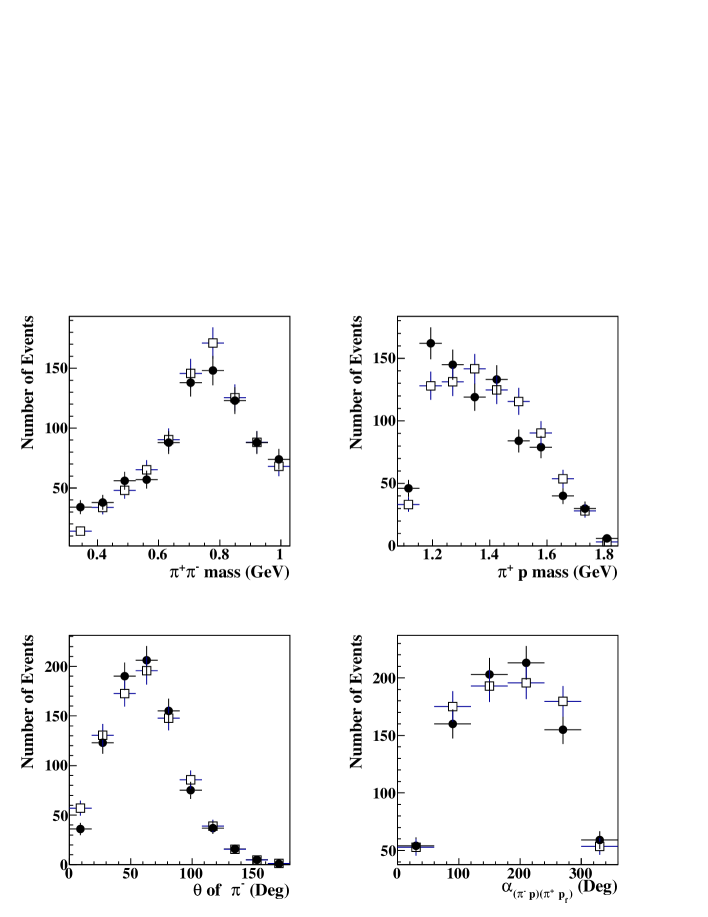
Figure 9: A comparison between the measured event distributions (solid circles) and the simulated event distributions (open squares) within the framework of the JM06 model Ripani et al. (2000); Mokeev et al. (2001); Aznauryan et al. (2005), which was further adjusted in order to reproduce the measured event distributions. These comparisons are shown for the bin of $W$=1.99 GeV and $Q^{2}$=4.6 GeV².

To obtain the 5-fold differential virtual photon cross sections in the blind areas we used:

• the number of measured data events (we weighted these events with the integral efficiency inside the 5-d bin) in the current $(W,Q^{2})$ bin, integrated over all hadronic variables for the $\pi^{+}\pi^{-}p$ final state $N_{data,int}$;

• the number of these events estimated from the event generator $N_{generated,int}$; and

• the number of generated events in a 7-d blind kinematic bin $(W,Q^{2},\tau_{i})$, which we call $N_{generated}^{7d}$.

Using the event generator as a guide, we interpolated the number of events measured outside of the blind bin into the blind bin. Thus, the number of counts for the 7-fold differential cross sections in the blind bins only were calculated by

$$\Delta N=\frac{N_{data,int}}{N_{generated,int}}N_{generated}^{7d},$$ (20)

and the 5-fold differential virtual photon cross sections in the blind bins were computed from $\Delta N$ in according to Eqs. (12-16), where we set $e\!f\!f=1$.

A comparison between the 1-fold differential cross sections obtained with and without generated events inside the blind bins is shown in Fig. 10. Except for the two bins of maximal CM $\theta_{\pi^{+}}$ angles, the difference between the two methods is rather small, and is inside the statistical uncertainties for most points. The estimated uncertainty introduced by this interpolation method has an upper limit of 5% on average, depending on the kinematics.

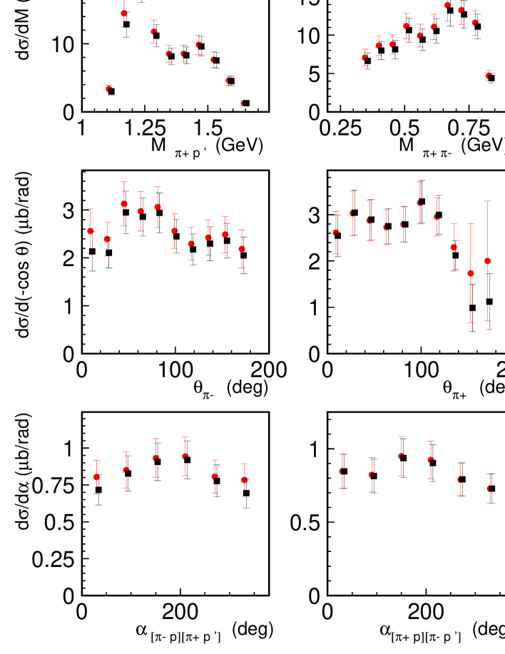
Figure 10: (Color online) Impact of the interpolation of the 5-fold $\pi^{+}\pi^{-}p$ differential cross sections into the blind areas of CLAS to the nine 1-fold differential cross sections at $W$=1.81 GeV and $Q^{2}$=2.6 GeV². The 1-fold differential cross sections obtained assuming zero 5-fold differential cross sections and the interpolated values for these cross sections in the blind areas of CLAS are shown by the black squares and red circles, respectively. The error bars represent statistical uncertainties. To aid visualization, we have slightly shifted horizontally the two data sets.

II.7 Radiative Corrections

To estimate the influence of radiative correction effects, we simulated $ep\to e^{\prime}\pi^{+}\pi^{-}p^{\prime}$ events using the above event generator both with and without radiative effects. For the simulation of radiative effects in double pion electroproduction, the well known Mo and Tsai procedure Mo and Tsai (1969) was used. As described above, we integrated the 5-fold two pion cross sections over four variables to get 1-fold differential cross sections. This integration considerably reduced the influence of the final state hadron kinematic variables on the radiative correction factors for the analyzed 1-fold differential cross sections. The radiative correction factor $R$ in Eq. (12) was determined as

$$R=\frac{N_{rad}^{2d}}{N_{norad}^{2d}},$$ (21)

where $N_{rad}^{2d}$ and $N_{norad}^{2d}$ are the numbers of generated events in each $(W,Q^{2})$ bin with and without radiative effects, respectively. We then fit the inverse factor $1/R$ over the $W$ range in each $Q^{2}$ bin. The factor $1/R$ for a representative bin 4.2 GeV² $<Q^{2}<5.0$ GeV² is plotted as a function of $W$ in Fig. 11. A few words should be said about the behavior of this factor. Since the radiation migrates events from lower $W$ to higher $W$, and because the structure at $W$ of around $1.7$ GeV is the most prominent feature of the cross sections, there is a small enhancing bump in the factor $1/R$ present in each $Q^{2}$ bin.

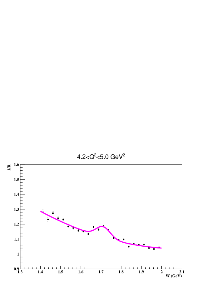
Figure 11: (Color Online) The radiative correction factor $1/R$ for the bin 4.2 GeV² $<Q^{2}<5.0$ GeV². The solid magenta line represents a polynomial plus Gaussian fit.

II.8 Systematic Uncertainties

One of the main sources of systematic uncertainty in this experiment is the uncertainty in the yield normalization factors, including the acceptance corrections, electron identification efficiency, detector efficiencies, and beam-target luminosity. The elastic events present in the data set were used to check the normalization of the cross sections by comparing the measured elastic cross sections to the world data. This allowed us to combine the luminosity normalization, electron detection, electron tracking, and electron identification uncertainties into one global uncertainty factor. In Fig. 12 the ratio of the elastic cross section to the Bosted parameterization Bosted (1995) is shown. The parameterized cross section and that from the CLAS elastic data are shown after accounting for radiative effects so that they are directly comparable. One can see most of the points are positioned within the red lines that indicate $\pm$10% offsets. This comparison allowed us to assign a conservative 10% point-to-point uncertainty to the full set of yield normalization factors for the two pion cross sections.

We restricted the $ep\to e^{\prime}\pi^{+}p^{\prime}X$ missing mass to be close to the $\pi^{-}$ peak in order to select two pion events. This missing mass cut event selection caused some loss of events. Uncertainties due to such losses were estimated by using Monte Carlo simulations for the acceptance calculations. The initial Monte Carlo distributions had better resolution than the data, so special CLAS software (GPP) was used to make them match. The uncertainty associated with the missing mass cuts was estimated by calculating the difference in the cross sections with two different missing mass cuts applied both on the real data and the Monte Carlo data sample. The missing mass cut used in the analysis was -0.04 GeV² $<M_{\pi^{-}X}^{2}<0.06$ GeV², so we varied the range of this cut to -0.02 GeV² $<M_{\pi^{-}X}^{2}<0.03$ GeV² to estimate the systematic uncertainty due to the missing mass cut.

We used the following method for estimating systematic uncertainties. In each case for a given observable ($e.g.$, mass distributions) we calculated the relative difference $(\sigma-\sigma_{c})/\sigma$, where $\sigma_{c}$ is the recalculated cross section with a more narrow missing mass cut. We expected to see a Gaussian-like distribution for the relative difference distribution. The difference between the centroid of this distribution and zero is a measure of the systematic uncertainty. From this, we estimated the systematic uncertainty due to the missing mass cuts at about 4.2% of the measured differential cross sections.

To estimate the influence of the detector fiducial area cuts, we recalculated the cross sections without applying fiducial cuts to the hadrons. Again, we constructed the relative difference $(\sigma-\sigma_{c})/\sigma$, where $\sigma_{c}$ is the recalculated cross section without hadron fiducial cuts. The result is that we saw a systematic decrease of about 2% in the cross sections.

We also varied the particle identification criteria, which included a cut on the calculated speed and momentum of the detected hadrons. In our analysis we applied a $\pm$2$\sigma$ cut, so to estimate the influence of these cuts to our results we recalculated cross sections with a $\pm$3$\sigma$ cut. By widening the particle identification cuts and using the same relative difference procedure as above, we saw a systematic increase of about 4.6% of the cross sections.

In addition, there were additional point-to-point uncertainties, dependent on the 5-d kinematics, due to the interpolation procedure to fill the blind bins. This systematic uncertainty for the 1-fold differential cross sections was estimated (from the differences shown in Fig. 10) to be on average 5% as an upper limit, but may be smaller in regions where the JM06 model gave a good representation of the measured cross sections and where we have only small contributions from filling blind areas of CLAS. Adding in quadrature the various systematic uncertainties, which were dominated by the normalization corrections, we found an overall systematic uncertainty of 14% for the cross sections reported here. The summary of the systematic uncertainties can be found in Table 1.

Sources of systematics	uncertainty, $\%$
Yield normalization	$10.0$
Missing mass cut	$4.2$
Hadron fiducial cuts	$2.0$
Hadron ID cuts	$4.6$
Radiative corrections	$5.0$
Event generator	$5.0$
Total	$14.0$

Table 1: Summary of sources of point-to-point systematic uncertainties for the cross section measurements reported in this work.

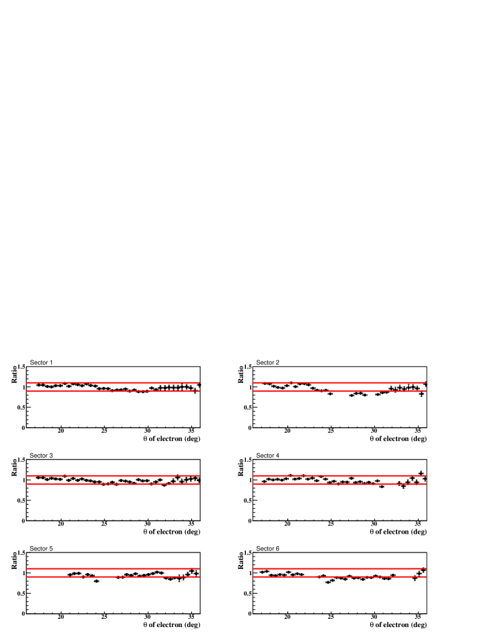
Figure 12: (Color Online) Ratio of the elastic cross section to the Bosted parameterization Bosted (1995) as a function of electron polar angle $\theta$ for each of the six sectors of CLAS. The regions where there are missing data are the result of $\theta$ vs. $p$ cuts to remove problematic areas of the detector. The horizontal lines represent $\pm$10% deviations of the ratio from unity.

III Results and Discussion

The fully integrated $\pi^{+}\pi^{-}p$ electroproduction cross sections obtained by integration of the 5-fold differential cross sections are shown in Fig. 13 for five $Q^{2}$ bins. Two structures located at $W$=1.5 GeV and 1.7 GeV produced by the resonances of the second and third resonance regions are the major features in the $W$ evolution of the integrated cross sections observed in the entire range of $Q^{2}$ covered by the CLAS measurements.

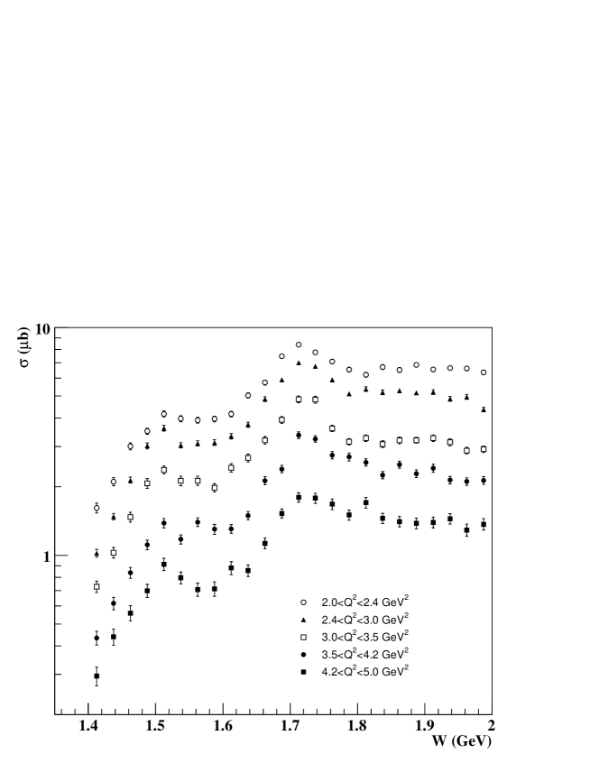
Figure 13: Fully integrated cross sections for $\pi^{+}\pi^{-}p$ electroproduction off protons at photon virtualities $Q^{2}$=2.2, 2.6, 3.2, 3.8, 4.6 GeV². The error bars represent the statistical uncertainties.

The results on the $\pi^{+}\pi^{-}p$ electroproduction cross sections discussed in Section II open up the possibility to extend our knowledge of the $\gamma_{v}pN^{*}$ electrocouplings of many resonances up to photon virtualities $Q^{2}=5$ GeV², in particular for the states in the mass range above 1.6 GeV Mokeev et al. (2016a, b), which decay preferentially to $\pi\pi N$ final states. This $Q^{2}$ range corresponds to the distance scale where the transition to the dominance of quark core contributions to the resonance structure takes place Aznauryan and Burkert (2012); Aznauryan et al. (2013); Segovia and others (2014); Segovia et al. (2015).

Here, we discuss the prospects for the extraction of resonance parameters from the new data based on comparisons between the measured nine 1-fold differential cross sections and the projected resonant contributions. Resonant contributions are computed within the framework of the recent JM model version Mokeev et al. (2009, 2012, 2016a) employing the unitarized Breit-Wigner ansatz for the resonant amplitudes described in Mokeev et al. (2012) and using interpolated resonance electrocouplings previously extracted in the analyses of exclusive meson electroproduction data from CLAS Aznauryan and Burkert (2012); Aznauryan et al. (2013); Park et al. (2015). This new version of the JM model is here referred to as JM16.

Exclusive meson	Nucleon	$Q^{2}$ ranges for extracted
electroproduction channels	resonances	$\gamma_{v}pN^{*}$ electrocouplings, GeV2
$\pi^{0}p$, $\pi^{+}n$	$\Delta(1232)3/2^{+}$,	0.16-6.00
	$N(1440)1/2^{+}$, $N(1520)3/2^{-}$, $N(1535)1/2^{-}$	0.30-4.16
$\pi^{+}n$	$N(1675)5/2^{-}$, $N(1680)5/2^{+}$	1.6-4.5
	$N(1710)1/2^{+}$	1.6-4.5
$\eta p$	$N(1535)1/2^{-}$	0.2-2.9
$\pi^{+}\pi^{-}p$	$N(1440)1/2^{+}$, $N(1520)3/2^{-}$	0.25-1.50
	$\Delta(1620)1/2^{-}$, $N(1650)1/2^{-}$, $N(1680)5/2^{+}$	0.50-1.50
	$\Delta(1700)3/2^{-}$, $N(1720)3/2^{+}$, $N^{\prime}(1720)3/2^{+}$	0.50-1.50

Table 2: Summary of the results on the nucleon resonance electrocouplings available from analyses of the CLAS exclusive meson electroproduction data off protons Mokeev et al. (2016a); Aznauryan and Burkert (2012); Aznauryan et al. (2009); Park et al. (2015); Mokeev et al. (2012); Mokeev and Aznauryan (2014).

Resonances	$\Gamma_{tot},$	Branching fraction	Branching fraction
	MeV	to $\pi\Delta$, %	to $\rho p$, %
$N(1440)1/2^{+}$	387	19	$1.7$
$N(1520)3/2^{-}$	130	25	$9.4$
$N(1535)1/2^{-}$	131	2	$10$
$\Delta(1620)1/2^{-}$	158	43	$49$
$N(1650)1/2^{-}$	155	5	$6$
$N(1680)5/2^{+}$	115	21	$13$
$\Delta(1700)3/2^{-}$	276	84	$5$
$N(1700)3/2^{-}$	148	45	$52$
$N^{\prime}(1720)3/2^{+}$	115	51	$9$
$N(1720)3/2^{+}$	117	39	$44$

Table 3: The nucleon resonances included in the evaluation of the resonant contributions to the $\pi^{+}\pi^{-}p$ electroproduction cross sections off protons, and their total decay widths and branching fractions for decays to the $\pi\Delta$ and $\rho p$ final hadron states used in the evaluation of the resonant contributions to the current measurements.

So far, $\gamma_{v}pN^{*}$ electrocouplings are available for excited nucleon states in the mass range up to 1.8 GeV. They were obtained from various CLAS data in the exclusive channels: $\pi^{+}n$ and $\pi^{0}p$ at $Q^{2}<5.0$ GeV² in the mass range up to 1.7 GeV, $\eta p$ at $Q^{2}<4.0$ GeV² in the mass range up to 1.6 GeV, and $\pi^{+}\pi^{-}p$ at $Q^{2}<1.5$ GeV² in the mass range up to 1.8 GeV. A summary of the results on the available resonance $\gamma_{v}pN^{*}$ electrocouplings can be found in Table 2. The $\gamma_{v}pN^{*}$ electrocoupling values, together with the appropriate references, are available from our web page Fedotov .

The $\gamma_{v}pN^{*}$ electrocouplings employed in the evaluations of the resonant contributions to the $\pi^{+}\pi^{-}p$ differential cross sections were obtained from interpolation or extrapolation of the experimental results Fedotov by polynomial functions of $Q^{2}$. The estimated resonance electrocouplings can be found in Isupov (2017). For low-lying excited nucleon states in the mass range $M_{N^{*}}<$ 1.6 GeV, the experimental results on the $\gamma_{v}pN^{*}$ electrocouplings are available at photon virtualities up to 5.0 GeV². Electrocouplings of these resonances were estimated by interpolating the data points. Electrocouplings of the $N(1675)5/2^{-}$, $N(1680)5/2^{+}$, and $N(1710)1/2^{+}$ resonances are available from $\pi^{+}n$ electroproduction data Park et al. (2015) at $Q^{2}$ from 2.0 GeV² to 5.0 GeV². To estimate their contributions to the $\pi^{+}\pi^{-}p$ electroproduction cross sections, we interpolated those results in $Q^{2}$.

Electrocouplings of the $\Delta(1620)1/2^{-}$, $\Delta(1700)3/2^{-}$, and $N(1720)3/2^{+}$ resonances are available at $Q^{2}<1.5$ GeV² Mokeev and Aznauryan (2014); Mokeev et al. (2016a, b). The recent combined analysis of the CLAS $\pi^{+}\pi^{-}p$ electroproduction off proton data Ripani et al. (2003) and the preliminary $\pi^{+}\pi^{-}p$ photoproduction data have revealed a contribution from a new candidate $N^{\prime}(1720)3/2^{+}$ state Mokeev et al. (2016b). This new $N^{\prime}(1720)3/2^{+}$ state and the existing $N(1720)3/2^{+}$ state with very similar masses and total hadronic decay widths, have distinctively different hadronic decays to the $\Delta\pi$ and $N\rho$ final states, and a very different $Q^{2}$-evolution of their associated electrocouplings. The resonant part of the $\pi^{+}\pi^{-}p$ electroproduction cross sections was computed by extrapolating the available results to the range of photon virtualities 2.0 GeV² $<Q^{2}<5.0$ GeV².

The contributions from resonances in the mass range above 1.8 GeV were not taken into account due to the lack of experimental results on their electrocouplings, thus limiting our evaluation of the resonant contributions to the range of $W<1.8$ GeV.

The hadronic decay widths to the $\pi\Delta$ and $\rho p$ final states for the above resonances were taken from previous analyses of the CLAS $\pi^{+}\pi^{-}p$ electroproduction data off protons Mokeev et al. (2012); Mokeev and Aznauryan (2014); Mokeev et al. (2016a, b). The constraints imposed by the requirement to describe $\pi^{+}\pi^{-}p$ electroproduction data with $Q^{2}$ independent hadronic decay widths for the contributing states, allowed us to obtain improved estimates of the branching fractions (BF) for the resonances listed in Table 3.

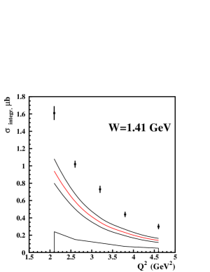
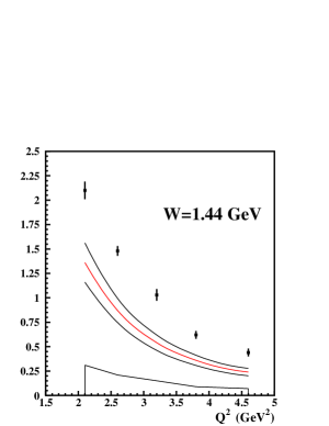
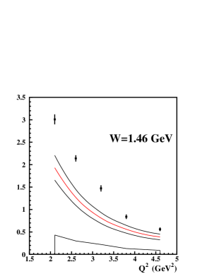
Figure 14: The resonant contributions from the JM16 model Mokeev et al. (2012, 2016a, 2016b) computed as described in Section III (red solid lines) in comparison with the CLAS results on the fully integrated $\pi^{+}\pi^{-}p$ electroproduction cross sections off protons (points with statistical error bars) in three $W$ bins near the central mass of the $N(1440)1/2^{+}$: $W$=1.41 GeV (left), $W$=1.44 GeV (center), and $W$=1.46 GeV (right). The systematic uncertainties of the measurements are shown by the bands at the bottom of each plot. The black lines that form a band about the central red JM16 prediction represent the model uncertainties.

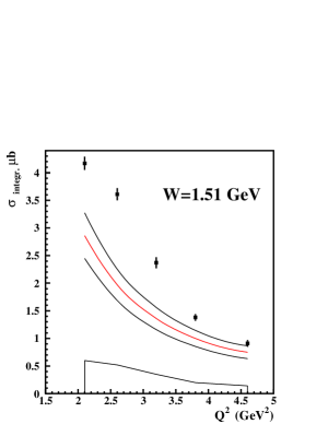
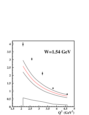
Figure 15: The resonant contributions from the JM16 model Mokeev et al. (2012, 2016a, 2016b) computed as described in Section III (red solid lines) in comparison with the CLAS results on the fully integrated $\pi^{+}\pi^{-}p$ electroproduction cross sections off protons (points with statistical error bars) in three $W$ bins near the central mass of the $N(1520)3/2^{-}$: $W$=1.51 GeV (left), $W$=1.54 GeV (center), and $W$=1.56 GeV (right). The systematic uncertainties of the measurements are shown by the bands at the bottom of each plot. The black lines that form a band about the central red JM16 prediction represent the model uncertainties.

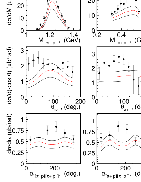
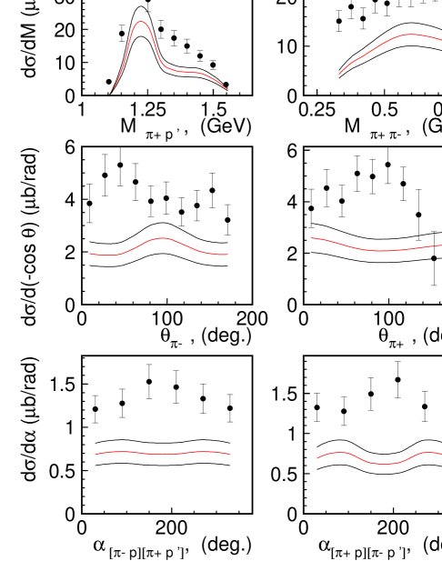
Figure 16: The resonant contributions from the JM16 model Mokeev et al. (2012, 2016a, 2016b) (red solid lines) to the nine 1-fold differential $\pi^{+}\pi^{-}p$ electroproduction cross sections in representative $W$ bins inside two $W$ intervals of distinctively different resonant content described in Section III at $Q^{2}$=2.1 GeV². The black lines that form a band about the central red JM16 prediction represent the model uncertainties.

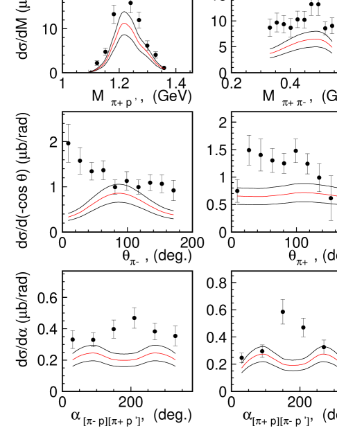
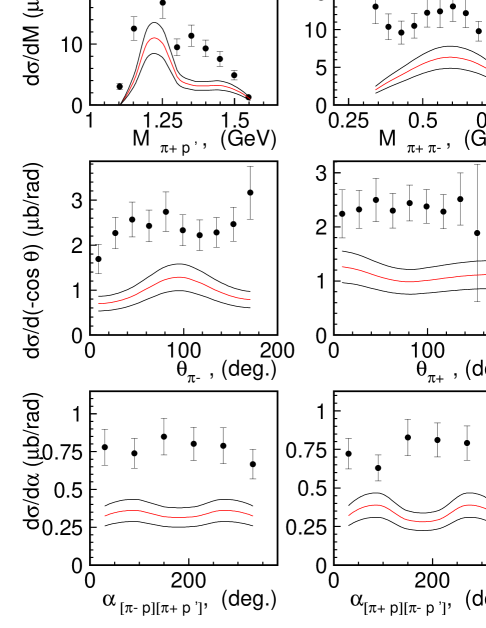
Figure 17: The resonant contributions from the JM16 model Mokeev et al. (2012, 2016a, 2016b) (red solid lines) to the nine 1-fold differential $\pi^{+}\pi^{-}p$ electroproduction cross sections in representative $W$ bins inside two $W$ intervals of distinctively different resonant content described in Section III at $Q^{2}$=3.2 GeV². The black lines that form a band about the central red JM16 prediction represent the model uncertainties.

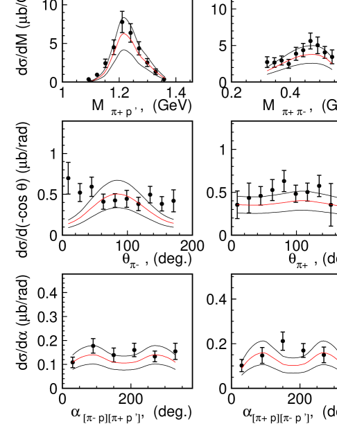
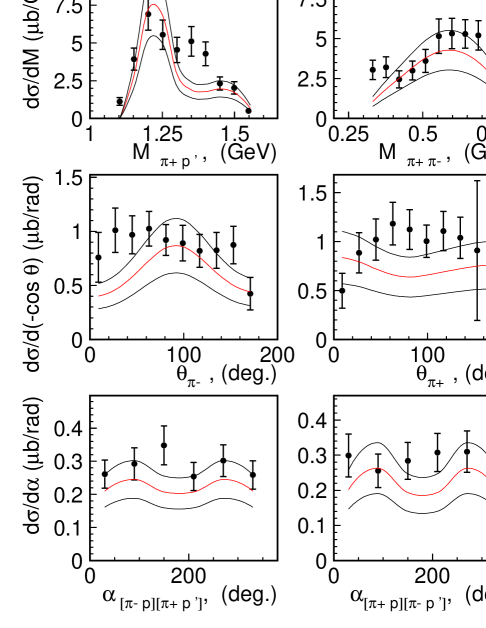
Figure 18: The resonant contributions from the JM16 model Mokeev et al. (2012, 2016a, 2016b) (red solid lines) to the nine 1-fold differential $\pi^{+}\pi^{-}p$ electroproduction cross sections in representative $W$ bins inside two $W$ intervals of distinctively different resonant content described in Section III at $Q^{2}$=4.6 GeV². The black lines that form a band about the central red JM16 prediction represent the model uncertainties.

The $Q^{2}$ dependence of the resonance contributions to the fully integrated $\pi^{+}\pi^{-}p$ electroproduction cross sections are shown in Figs. 14 and 15. The data shown correspond to the $W$ ranges that are closest to the central masses of the $N(1440)1/2^{+}$ and $N(1520)3/2^{-}$. The electrocouplings of these low-lying resonances, as well as for the $N(1535)1/2^{-}$, are available in the entire range of $Q^{2}$ covered in our measurements Denizli et al. (2007); Aznauryan et al. (2009); Mokeev et al. (2012); Park et al. (2015); Mokeev et al. (2016a). Interpolated values of these electrocouplings were used in the resonant contribution evaluations shown in Figs. 14 and 15. In the mass range from 1.50 GeV to 1.56 GeV, there is also a small contribution from the tail of the $\Delta(1620)1/2^{-}$ resonance. Electrocouplings of this resonance are available at $Q^{2}<1.5$ GeV² Mokeev et al. (2016a). To evaluate this contribution, the CLAS results were extrapolated into the range 2.0 GeV² $<Q^{2}<5.0$ GeV².

The uncertainties of the resonant contributions were estimated from the quadrature sum of the statistical and systematic uncertainties of the measured integrated cross sections, assuming that the relative uncertainties both for the fully integrated and all 1-fold differential cross sections were the same for the measured cross sections and for the computed resonant contributions, as was found in previous analyses of $\pi^{+}\pi^{-}p$ electroproduction data from CLAS Mokeev et al. (2012, 2016a). Under this assumption, the initial evaluation of the uncertainties for the resonant contributions was performed accounting for only statistical uncertainties of the measured integrated and 1-fold differential cross sections. However, the statistical uncertainties offer a reasonable estimate only in the case when the $\chi^{2}/d.p.$ ($\chi^{2}$ per data point) achieved in the data fit is close to unity. The $\chi^{2}/d.p.$ values achieved in the previous analyses of the CLAS $\pi^{+}\pi^{-}p$ electroproduction data were in the range from 1.3 to 2.9 Mokeev et al. (2012, 2016a, 2016b). In order to account for the additional data uncertainties responsible for the deviation of the $\chi^{2}/d.p.$ values from unity, we multiplied the initial values of the uncertainties for the resonant contributions by the root square of the averaged $\chi^{2}/d.p.$ value achieved in the previous data fits, which was equal to 1.45. Uncertainties of the estimated resonant contributions to the fully integrated $\pi^{+}\pi^{-}p$ electroproduction cross sections are represented in Figs. 14 and 15 by the areas between the black solid lines.

The results shown in Figs. 14 and 15 demonstrate an increase with $Q^{2}$ of the relative resonance contributions to the fully integrated $\pi^{+}\pi^{-}p$ electroproduction cross sections. The resonant part begins to dominate at $Q^{2}>4.0$ GeV². Table 4 shows ratios of the projected resonant contributions to the measured cross sections in several $Q^{2}$ bins averaged within three $W$ intervals that have distinctively different resonant content.

• In the interval 1.41 GeV $<W<1.61$ GeV, electrocouplings of the low-lying resonances have been measured in the $Q^{2}$ range covered here.

• For the states in the mass range 1.61 GeV $<W<1.74$ GeV that contribute to the $\pi^{+}\pi^{-}p$ electroproduction, only electrocouplings of the $N(1685)5/2^{+}$ resonance are available from the CLAS $\pi N$ data Park et al. (2015) in the range of $Q^{2}$ covered in our measurements. The $\Delta(1620)1/2^{-}$, $\Delta(1700)3/2^{-}$, $N(1720)3/2^{+}$, and candidate $N^{\prime}(1720)3/2^{+}$ states decay preferentially to $\pi\pi N$. Their contributions, as well as from the $N(1650)1/2^{-}$ to the $\pi^{+}\pi^{-}p$ cross sections, have been evaluated by extrapolating the available electrocouplings from $Q^{2}<1.5$ GeV² Mokeev et al. (2016b) to 2.0 GeV${}^{2}<Q^{2}<5.0$ GeV².

• The interval 1.74 GeV $<W<1.82$ GeV includes only states recently reported Particle Data Group, K. A. Olive et al. (2014) for which no electrocouplings are available to date, and their $\pi\pi N$ couplings are also unknown. Hence no projections are possible in this mass range. No resonances in this mass range were included for evaluation of the resonant contributions to the $\pi^{+}\pi^{-}p$ electroproduction cross sections.

$Q^{2}$,	1.41 $<$ $W$ $<$ 1.61,	1.61 $<$ $W$ $<$ 1.74,	1.74 $<$ $W$ $<$ 1.82,
GeV2	GeV	GeV	GeV
2.1	0.650 $\pm$ 0.033	0.570 $\pm$ 0.034	0.200 $\pm$ 0.019
2.6	0.570 $\pm$ 0.029	0.500 $\pm$ 0.028	0.180 $\pm$ 0.010
3.2	0.550 $\pm$ 0.029	0.490 $\pm$ 0.029	0.190 $\pm$ 0.017
3.8	0.660 $\pm$ 0.034	0.620 $\pm$ 0.034	0.210 $\pm$ 0.014
4.6	0.750 $\pm$ 0.041	0.790 $\pm$ 0.049	0.240 $\pm$ 0.017

Table 4: Ratios of the resonant contributions computed within the framework of the current JM16 model version Mokeev et al. (2012, 2016a, 2016b) relative to the measured fully integrated $ep\to e^{\prime}\pi^{+}\pi^{-}p^{\prime}$ cross sections averaged within three $W$ intervals with different resonant content.

In Figs. 16, 17, and 18 we show the comparison of the nine 1-fold differential $\pi^{+}\pi^{-}p$ electroproduction cross sections and the resonant contributions computed in the JM16 model within the given $W$ and $Q^{2}$ bins. The resonant contributions obtained with the resonant parameters of the JM16 model taken from previous analyses of the CLAS $\pi^{+}\pi^{-}p$ electroproduction data at $Q^{2}<1.5$ GeV² Mokeev et al. (2012, 2016a) after interpolation/extrapolation of the $\gamma_{v}pN^{*}$ electrocouplings to the $Q^{2}$ range covered in our measurements, are shown by the red lines. The uncertainties for the resonant contributions were evaluated as described above. The procedure for the evaluation of the resonant contributions to the 1-fold differential cross sections within the framework of the unitarized Breit-Wigner ansatz is described in Mokeev et al. (2012, 2016a). The uncertainties in the resonant contributions to the 1-fold differential cross sections are shown in Figs. 16, 17, and 18 by the areas between the black solid lines.

According to the results in Figs. 16, 17, and 18, the projected resonance contributions to the measured cross sections at $W<1.74$ GeV are the largest over the entire $Q^{2}$ range covered here as shown in Table 4. We find that the relative resonant contributions increase with $Q^{2}$ and dominate the integrated cross section in the highest $Q^{2}$ bin centered at 4.6 GeV².

However, the resonant contributions to the CM angular distributions at $Q^{2}=4.6$ GeV² and in the mass range 1.51 GeV to 1.71 GeV shown in Fig. 18 indicate sizable differences in the angular dependence of the measured differential cross sections and the projected resonance contributions. This suggests substantial contributions from non-resonant mechanisms even at the highest photon virtualities covered by our measurements.

In particular, a comparison of the measured CM angular distributions for the final state $\pi^{-}$ and the computed resonant contributions shown in Fig. 18 suggests that the non-resonant contribution from the $\pi^{-}\Delta^{++}$ intermediate state created in the $t$-channel exchange dominates at forward angles. Also, the presence of a direct $2\pi$ production mechanism may explain the differences between the measured cross sections and the resonant contributions seen at the backward $\pi^{-}$ angles.

In the $W$ interval from 1.74 GeV to 1.82 GeV the ratio of the projected resonant contributions to the fully integrated $\pi^{+}\pi^{-}p$ electroproduction cross sections decreases by more than a factor of two in all $Q^{2}$ bins covered here (Table 4). In order to achieve a satisfactory description of the data in this mass range with the resonant contributions from the aforementioned resonances only, requires an increase of the relative contribution from the non-resonant mechanisms by more than a factor of two, which seems unlikely.

The data discussed here therefore present an opportunity to independently verify signals from new baryon states reported in the Bonn-Gatchina photoproduction data analysis Anisovich et al. (2012). A successful description of the $\pi^{+}\pi^{-}p$ photo- and electroproduction data with $Q^{2}$-independent resonance parameters (such as partial $\pi\Delta$ and $\rho p$ decay widths) would provide strong evidence for these newly claimed excited nucleon states.

According to Table 4, at $W$ $<$ 1.74 GeV the relative resonant contributions decrease in the $Q^{2}$ range from 2.0 GeV² to 3.0 GeV², while at $Q^{2}>3.0$ GeV² the relative resonant contributions exhibit an increase with $Q^{2}$. For resonances in the mass range from 1.41 GeV to 1.61 GeV, the electrocouplings are known from CLAS data in the entire range of photon virtualities covered by our measurements. Therefore, this effect cannot be related to uncertainties resulting from the extrapolations of the resonance electrocouplings.

Our data suggest that at $Q^{2}<3.0$ GeV² the resonance contributions decrease with $Q^{2}$ faster in comparison with other contributing mechanisms. Instead, at $Q^{2}>3.0$ GeV² the resonance contributions decrease with $Q^{2}$ slower in comparison with the remaining contributions to exclusive $\pi^{+}\pi^{-}p$ electroproduction. Such behavior supports the assessment of the structure of the $N^{*}$ states from analyses of exclusive meson electroproduction Aznauryan and Burkert (2012); Mokeev et al. (2016a) as an interplay of the inner core of three dressed quarks and the external meson-baryon cloud. The range of $Q^{2}<3.0$ GeV² corresponds to substantial contributions from the meson-baryon cloud, which becomes largest at the photon point. This contribution decreases with $Q^{2}$ faster than the contribution from non-resonant mechanisms and its relative resonant contribution decreases with $Q^{2}$ for $Q^{2}<3.0$ GeV². Instead, at higher $Q^{2}$ the contribution from the quark core becomes more significant, even dominant, and this contribution decreases with $Q^{2}$ more slowly than the non-resonant processes, causing relative growth of the resonant cross sections.

IV CONCLUSIONS

In this paper we presented new electroproduction data on $ep\to e\pi^{+}\pi^{-}p^{\prime}$ in the mass range $W<2.0$ GeV, and at photon virtualities 2.0 GeV² $<Q^{2}<5.0$ GeV². The kinematics covered is rich with known nucleon resonances whose electrocouplings are either unknown or known from $\pi N$ electroproduction only. In particular, these data cover the range of $W>1.6$ GeV, where many resonances couple predominantly to the $\pi\pi N$ final state, and hence can be studied here.

The extraction of the electrocoupling amplitudes requires a reaction model that must include all well established resonances in amplitude form, along with the amplitudes of the relevant non-resonant mechanisms and the interference of the contributing amplitudes. One such model is the JM framework Mokeev et al. (2012, 2016a, 2016b), but its reach in the invariant mass of the final hadrons $W$ and photon virtuality $Q^{2}$ must be extended into the kinematic domain of the new data. This effort is underway and the results will be part of a future publication on the subject.

The projected resonant contributions to the cross sections discussed in Section III were obtained within the framework of the unitarized Breit-Wigner ansatz of the JM16 version of the JM model Mokeev et al. (2012). The resonant cross sections were evaluated with electrocouplings determined by interpolations and extrapolations of the available results on these resonance parameters Isupov (2017); Fedotov from the measured $Q^{2}$ into new territory.

Our studies show strong indications that the relative contributions of the resonant cross section at $W<1.74$ GeV increase with $Q^{2}$. This suggests good prospects for the exploration of electrocouplings of the nucleon resonances in this mass range and with photon virtualities up to 5.0 GeV² and above. With the CEBAF accelerator upgrade to an energy of 12 GeV and by employing the new CLAS12 detector, photon virtualities in the range 5.0 GeV${}^{2}<Q^{2}<12.0$ GeV² can be reached for all of the prominent resonances with masses below 2.0 GeV. The range of $Q^{2}>2.0$ GeV² is of particular importance to study the momentum dependence of the light-quark masses, as the $Q^{2}$ dependence of the resonance electrocouplings has been shown to be sensitive to the quark mass function Roberts (2016, 2016). This provides a sensitive means of testing computations of the electrocouplings from first principles QCD as incorporated in the Dyson-Schwinger equation (DSE) approach Segovia and others (2014); Segovia et al. (2015).

The data presented here provide a basis to verify the existence of possible new baryon states reported at $M>1.8$ GeV in a global multi-channel partial wave analysis of photoproduction data by the Bonn-Gatchina group Anisovich et al. (2014). The apparent decrease in the resonant contributions at $W>1.74$ GeV, as shown in Table 4, suggests that more resonances in this mass range will be needed to describe the present data, as well as the possibility to locate new baryon states by examining these data with $Q^{2}$ independent hadronic parameters for the excited nucleon states. In addition, reaching higher mass states at 2 GeV and above will allow us to test the quark model predictions employing light-front dynamics Aznauryan and Burkert (2015) and other approaches Santopinto and Giannini (2015) in a domain where first principles calculations are still unavailable.