Entanglement entropy and Fisher information metric for closed bosonic strings in homogeneous plane wave background
Abstract
We derive the extended renormalized entanglement entropy (EREE) and the Fisher information metric in the case of closed bosonic strings in homogeneous plane wave background. Our investigations are conducted within the framework of Thermo Field Dynamics (TFD). The formalism is also illustrated on the example of some particular models in condensed matter physics and the non-equilibrium case for system with dissipations.
Keywords: Thermo field dynamics, entanglement entropy, Fisher metric, string theory
1 Introduction
Entanglement entropy (EE) is a measure of how much information is stored in a quantum system. One expects that EE is directly related to the degrees of freedom. In this sense it can be used to gain insight into the quantum dynamics of diverse and complex phenomena. In recent years it also became a powerful bridge between string/gravity and condensed matter physics. For example, in holographic systems, the entanglement entropy is encoded in the geometric features of different string backgrounds [1, 2]. This is closely related to the concept of
emergent spacetime in such models [3, 4, 5]. The progress so
far suggests that one can also study relevant aspects of string theory on microscopic level by making use of thermodynamic and information-theoretic quantities.
Our interest is focused specifically on the study of quantum entanglement entropy and the Fisher information for particular string model, namely closed bosonic strings on homogeneous plane wave backgrounds. In general it is difficult to calculate the entanglement entropy, especially in quantum field theory on curved spacetime. However, the recent progress in thermo field dynamics [6, 7, 8, 9, 10] offers relatively easy and straightforward way of treating quantum states, which facilitates the derivation of the EE and the Fisher matrix for the relevant models considered in this paper.
Thermo field dynamics requires a “statistical” state defined in a double Hilbert space, which is a direct product of the original space and an isomorphic copy of it. If one chooses to work in the energy basis , where , , then the bases in the double Hilbert space are labelled as . The extended states were defined originally by [8, 9, 6]:
| (1.1) |
where is the partition function. It was shown in [11] that the extended state is invariant for any orthogonal complete set , . Thus the statistical state is independent of the chosen representation. This result is known as “the general representation theorem” in TFD. It allows one to use TFD techniques even in the non-equilibrium case. The notion of double Hilbert space is very useful in treating quantum states directly and facilitates the calculation of entanglement entropy of the quantum systems. Although TFD works for arbitrary non-diagonal Hamiltonians the calculations simplify if one is allowed to work only with diagonal Hamiltonians, which is the case we prefer in this study.
Let the Hamiltonian be a bilinear function in creation and annihilation operators. One can diagonalise
it by an appropriate procedure, commonly known as the Bogoliubov transformation [12, 13]. It mixes the creation and annihilation operators, but leaves the form of the commutation relations unchanged. In this case operator eigenvalues, calculated with the diagonalized Hamiltonian on the transformed state functions, remain unchanged. Many such examples exist with important applications in condensed matter physics and string theory.
This paper is structured as follows. In section 2 we consider rather generic case of a system in equilibrium, where one applies TFD techniques to calculate the extended entanglement entropy and the Fisher information metric. In section 3 we show that our result is applicable for certain bosonic and fermionic systems, naturally found in condensed matter systems such as superfluidity, superconductivity and spin chains. In section 4 we calculate the EREE and the Fisher metric for a non-trivial example of closed bosonic string theory in a class of curved plane wave backgrounds. In section 5 we consider a non-equilibrium case with dissipation and generalize the formula for EREE found in [14]. Finally, in section 6 we make a short summary of our results.
2 Entanglement entropy for time-independent quadratic Hamiltonians
2.1 Extended entanglement entropy for systems in equilibrium
Let be a complete basis of eigenfunctions of the operator ,
| (2.1) |
In general the Hamiltonian in such a basis is non-diagonal,
| (2.2) |
where the creation and annihilation operators satisfy standard commutation relations,
| (2.3) |
If the Hamiltonian is diagonalizable one can write it in the following form [12, 13, 15]111For more general discussion on quantum quadratic Hamiltonians see the lecture notes [16].
| (2.4) |
where the energy coefficients and the energy of the ground state depend on the matrix elements of the original Hamiltonian (2.2). The new creation and annihilation operators and satisfy the same commutation relations as the previous operators and :
| (2.5) |
Following [14, 17] we can apply TFD techniques to find the EREE for the new system of quasi-particles, described by the Hamiltonian (2.4). Consider the excited states , which satisfy the orthonormal relation
| (2.6) |
One can write the Hamiltonian in matrix form such as222Let us clarify the notations to avoid unnecessary confusion. If we define , then a non-diagonal Hamiltonian can be written in the form The last expression allows one to write as a matrix, where and run over all possible states, defined by the quantum numbers (for explicit examples see [17, 18]).
| (2.7) |
where are the number operators, . Once the Hamiltonian assumes diagonal form it is straightforward to compute the relevant statistical quantities. The first one is the partition function ,
| (2.8) |
where , and , (). We also introduce the notations and , , usually called inverse scaled temperatures. The ordinary density matrix in equilibrium is given by
| (2.9) |
In order to define the entanglement entropy the whole system is divided into two subsystems and , traditionally called “Alice” and “Bob”. Then, the standard EE for the first system is found as333We prefer to work in units , where is the Boltzmann constant.
| (2.10) |
In the TFD formulation of the double Hilbert space the statistical state, , is defined as
| (2.11) |
Thus the extended density operator assumes the form
| (2.12) |
One can choose a bipartite system, namely
| (2.13) |
The extended density matrix for “Alice” is obtained as a trace over the parameters of the second system ,
| (2.14) |
which leads to
| (2.15) |
Finally, the extended renormalized entanglement entropy, , follows as
| (2.16) |
The result simplifies in terms of hyperbolic functions:
| (2.17) |
This is the desired expression for the EREE. If the formula reduces to (3.14). If , it reproduces the result for the EE of the Pais-Uhlenbeck oscillator, found in [19]. For comparison the standard entanglement entropy from (2.10) is written by
| (2.18) |
2.2 Fisher information metric
Equation (2.17) allows one to calculate the Fisher information metric. It can be expressed as a second derivative of the entanglement entropy [20, 21]:
| (2.19) |
where and
| (2.20) |
| (2.21) |
| (2.22) |
| (2.23) |
| (2.24) |
| (2.25) |
Formula (2.19) differs by a sign from the standard definition of the metric due to the requirement that the metric components be positive defined, which is a necessary condition for thermodynamic stability (for extended discussion see [22] and references therein). The case of corresponds to the Fisher metric obtained by [19, 23].
On the level of the space of probability distributions the Fisher metric represents a continuous setting even if
the underlying features of the system (for example, the state space) are discrete. This allows one to take advantage of the powerful framework
of differential geometry to treat statistical structures as geometrical
ones. As it turns out the expressions for the EE and Fisher metric are applicable for variety of system as shown below.
3 Examples from condensed matter physics
Diagonalizable or approximately diagonalizable bosonic and fermionic Hamiltonians naturally arise in condensed matter physics such as spin wave theory, Heisenberg ferro- and anti-ferromagnets, spin chains, spin liquids, BCS theory of superconductivity [24], but also in quantum field theory and string theory. In this section we give explicit examples of EREE for bosonic and fermionic systems, correspondingly.
3.1 Entanglement entropy for bosonic system
For simplicity let us consider the following BCS type bosonic Hamiltonian:
| (3.1) |
where , and are some energy coefficients and
| (3.2) |
Following [12], we want to transform the given Hamiltonian by introducing new set of operators and , such that (3.1) takes the following diagonal form:
| (3.3) |
Here, the creation and annihilation operators and also satisfy (3.2),
| (3.4) |
The diagonalization is achieved by the following Bogoliubov transformations:
| (3.5) |
After some trivial calculations one arrives at the following expressions for the new Hamiltonian coefficients:
| (3.6) |
| (3.7) |
| (3.8) |
where is the energy of the ground state. Now, let us focus on the calculation of the EREE for the system described by the Hamiltonian (3.3). First we calculate the partition function
| (3.9) |
The ordinary equilibrium density matrix is written by
| (3.10) |
where , , are the number operators of the Bogoliubov quasi-particles. The TFD statistical state, , is defined as
| (3.11) |
Therefore, the extended density operator, , takes the form
| (3.12) |
Tracing out the states of the second system, one finds
| (3.13) |
Finally, the renormalized extended entanglement entropy for the given bosonic system is written by
| (3.14) |
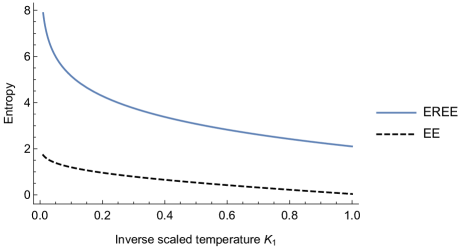
Here is the inverse scaled temperature. As expected the result agrees with eq. (2.17) for . The dependence of the entropy on is illustrated on figure 1.
In this case the Fisher information (2.19) is a one parameter function given by
| (3.15) |
It measures the amount of
information that an observed random variable provides about
an unknown parameter. It can be used in studying phase transitions, especially
the second-order phase transitions, during which the Fisher
information exhibits divergence. From eq. (3.1) one notices that Fisher information is singular at the origin . This suggest that at very high temperatures the Bogoliubov quasi-system undergoes a second-order phase transition, which is in agreement with the statement that the Fisher information is maximized at the phase transition points [25].
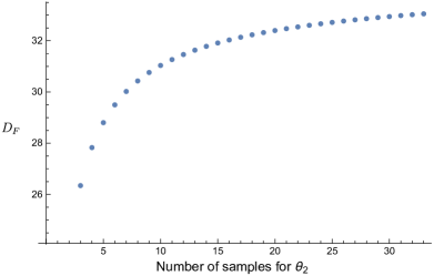
One can use the Fisher information (3.1) to define a distance between points on the statistical manifold, spanned by the inverse scaled temperatures , or in this case – only by . The information-metric distance, or Fisher information distance [26], , between two distributions and in a single parameter family is defined by
| (3.16) |
where and are parameter values corresponding to the two PDFs. On figure 2 are depicted several values of the Fisher distance for several increasing positive values of the upper integral limit , while keeping the lower limit fixed. This setup chooses different points on the statistical manifolds. One notices that increases monotonously for increasing values of the upper limit . For nearby states, the square of the lengths of the geodesic paths gives the probability of a fluctuation between the states. In other words, the less the probability of a fluctuation between two states, the further apart they are [22].
3.2 Entanglement entropy for fermionic system
In this section we are going to consider a fermionic example, namely XY model in a magnetic field. It is a generalization of the Ising model in which an anisotropy is introduced with respect to the x and y directions by means of a real deformation parameter . In what follows we are going to shortly sketch the diagonalization of the Hamiltonian, which is given by [27]:
| (3.17) |
Here gives the total odd number of spins and is the transverse magnetic field. In the case the system reduces to the one-dimensional Ising model with transverse magnetic field. In order to diagonalize the Hamiltonian we begin by defining the following operators:
| (3.18) |
Next we perform the Jordan-Wigner transformation, which relates the spin operators to a set of fermionic operators and via
| (3.19) |
Here the operators and satisfy the standard fermionic anticommutation relations:
| (3.20) |
The Hamiltonian, written in terms of these fermionic operators, assumes the form
| (3.21) |
Now we Fourier transform the creation and annihilation operators by
| (3.22) |
where . The Hamiltonian is expressed as
| (3.23) |
After applying the following Bogoliubov transformations:
| (3.24) |
one finds
| (3.25) |
Imposing that the cross-terms be zero we arrive at the expressions relating with the original parameters ():
| (3.26) |
Finally, the Hamiltonian assumes the form of a quasi-free fermionic system:
| (3.27) |
where defines number operators for the quasi-particles and sets the following dispersion relation:
| (3.28) |
One can repeat the TFD analysis from section 2 to calculate the extended entanglement entropy, which, for arbitrary number of spins , coincides with equation (2.17):
| (3.29) |
where the inverse scaled temperatures are given by . Here we used natural numbers to count the number of spins involved. In such notations one has to be careful with the expressions for and , where , and the angle . This implies the following relation , thus
| (3.30) |
The Fisher information metric in this case is the same as in section 2 for particular values of .
4 Entanglement entropy for closed bosonic strings in homogeneous plane wave backgrounds
In this section we consider the closed bosonic string vibrating in regular homogeneous plane-wave backgrounds. The given curved backgrounds have non-vanishing NS three-form field strength and a dilaton. We will closely follow [28], where the authors develop a general procedure for solving linear, but non-diagonal equations for the string coordinates, and determine the corresponding oscillator frequencies and the light-cone Hamiltonian. In this set up the Hamiltonian is automatically diagonalized and time-independent. Therefore, finding the entanglement entropy in the framework of TFD naturally follows the steps shown in the previous sections. Bellow we will sketch the relevant result of [28].
4.1 String equations of motion and quantization
We begin by considering a closed relativistic string in non-singular dimensional homogeneous plane-wave backgrounds with metric of the following form
| (4.1) |
Here and are constant, and the -field is given by . Our aim is to solve the classical equations of motion for this string sigma model. We denote the string embedding coordinates as . Choosing the orthogonal gauge for the world-sheet metric, the standard sigma model Lagrangian is written by
| (4.2) |
The equations of motion for the bosonic field are easily obtained:
| (4.3) |
Similarly, for the fields , , one finds
| (4.4) |
where and . In the light-cone gauge becomes
| (4.5) |
where the condition of periodicity of in implies that . To solve eq. (4.4) one makes the following mode expansion of the transverse coordinates
| (4.6) |
The substitution of the mode expansion in eq. (4.4) leads to
| (4.7) |
For simplicity one can set and assume that is diagonal, . As explained in [28], the general method to solve systems like (4.7) is to rewrite it as a set of first-order equations and then use the appropriate methods available at hand. Fortunately, the authors noted that for generic values of the parameters in (4.7) one can use a much simpler procedure. Namely, to solve these equations, one makes the following ansatz:
| (4.8) |
with the frequencies and their eigen-directions to be determined. This frequency based ansatz for the modes leads to the matrix equation in the form
| (4.9) |
where (for short ):
| (4.10) |
The matrix equation (4.9) is a homogeneous algebraic system. The necessary condition for finding a non-trivial solution is
| (4.11) |
The later equation has roots , , which are the frequencies from (4.8). The ansatz (4.8) is justified only if all the roots are distinct, or if equal roots are associated with linearly independent null eigenvectors, because it involves all the linearly independent solutions of the equation (4.7). The degenerate case requires separate considerations. In what follows we will always assume distinct roots. From (4.10) one immediately notes that . This property means that and have the same determinant and hence the same roots. This leads to the situation where for the frequencies come in pairs, . It is then convenient to rewrite the expansion of the zero-mode as
| (4.12) |
For the higher modes () the modes are paired, , . It is useful to chose the eigen-directions in the following way:
| (4.13) |
where , , are the minors of the matrix , evaluated for . Therefore one can rewrite the solution for the string modes explicitly as
| (4.14) |
| (4.15) |
In order to find the Hamiltonian we promote the ’s to operators with commutation relations given by
| (4.16) |
where one has
| (4.17) |
The expressions for these coefficients follow from the canonical equal-time commutation relations between the string modes . The relations between the ’s and the canonically normalised operators , , are given by
| (4.18) |
where . With this choice for the ’s the bilinear combination is related to the number operator, , by
| (4.19) |
Similar relation holds for the higher modes,
| (4.20) |
which connects the number operator with the operators. Hence, one has an explicit string mode expansion. Thus, the string Hamiltonian,
| (4.21) |
can be written as a sum of -level harmonic oscillator Hamiltonians
| (4.22) |
Here the zero-mode part Hamiltonian assumes the form
| (4.23) |
with frequencies
| (4.24) |
Likewise, the Hamiltonians for higher modes of the string are given by
| (4.25) |
where the frequency is a sum of two terms – one coming from the plane wave metric, and the other coming from the Kalb-Ramond B-field:
| (4.26) |
4.2 Extended entanglement entropy in the ground state of the bosonic string
We are now ready to apply the TFD technique for the entanglement entropy on every energy level of the string spectrum. Here, for convenience, we consider only the Hamiltonian of the string from eq. (4.23). Assume the following two subsystems:
| (4.27) |
the resulting entanglement entropy agrees with equation (2.17):
| (4.28) |
The thermal parameters, , depend on the frequencies of the classical string modes , . In four-dimensional spacetime , thus , the space of parameters is one-dimensional spanned by the values of . The entanglement entropy behaves as shown in figure 1. In 5-dimensions (, ), the space of parameters is a two-dimensional Riemannian manifold spanned by . The the entanglement entropy is given by
| (4.29) |
The inverse scaled temperatures, , depend on the sign of the coefficients , which leads to two regions on the plot (fig. 3) – one for positive values of the ’s, and one for negative ones.
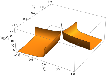
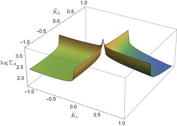
As expected for very high temperatures () the entropy diverges. One finds similar situation for the standard entanglement entropy,
| (4.30) |
shown in figure 4 below,
The Fisher metric, , at the point (), is also singular, as can be seen from the following expressions for the metric coefficients:
| (4.31) | ||||
| (4.32) | ||||
| (4.33) |
This result is already familiar [19]. The singular point at the origin is a signal of a phase transition. As shown from the geometric analysis of the Fisher metric in section 4.3 its Ricci scalar is regular at the origin, which suggests that the point () is not a second order phase transition. Furthermore, the scalar curvature at that point is zero, corresponding to a free quasi-system at very high temperatures.
4.3 Geometric analysis of the Fisher metric and phase transitions
Well-known fact is that the Fisher information metric defines a Riemannian metric on the space of parameters [29, 30, 31] for variety of statistical systems. Such geometrization is often useful in the analysis of the phase structure for a given statistical model [32, 22]. Here the scalar curvature, , plays a central role, e.g. a non-interacting model shows a flat geometry (), while diverges at the critical points of an interacting one, thus effectively preventing
geodesics from crossing into the nonphysical area of phase space [33, 34, 35, 36]. The specific critical points, where the phase transition occurs, lie on the spinodal curve. An advantage of the probabilistic description of the system’s phase structure is that one does not require the definition of order parameters. This is useful for systems where an order parameter is difficult to identify, or does not exist.
In what follows we analyse the scalar curvature of the Fisher metric from (4.2), (4.2) and (4.2). The scalar curvature is independent of the chosen coordinates, so, for convenience, we perform a change of variables from and to and . The Fisher metric in the new coordinates is given by
| (4.34) | |||
| (4.35) | |||
| (4.36) |
where and
| (4.37) |
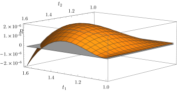
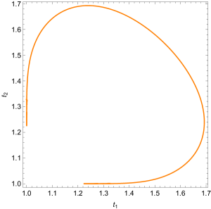
The explicit expression for is too lengthy to be presented here. However its functional dependence on () near the origin (1,1) is shown on figure 5. One notes that the Ricci scalar is positive defined and shows local maximum near the point (). The positive values of the scalar curvature suggest elliptic geometry in the thermodynamic parameter space, while the local maximum corresponds to the strongest interaction between the constituents of the quasi-system. There is a level curve for which , corresponding to free non-interacting system (fig. 6). At the origin the scalar curvature is also regular and tends to zero, which implies that the singular point in the Fisher metric is not a second-order phase transition and also shows that at very high temperatures the system is free. One notes that the values of do not deviate much from zero, which makes the entire quasi-system almost non-interacting. This kind of behaviour is expected due to the properties of the Bogoliubov transformation, which smoothens out the strength of the interactions in the original quantum system and effectively produces a non-interacting quasi-system.
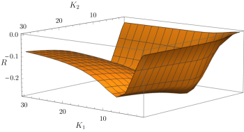
For larger values of the parameters the Ricci scalar is not positive defined as shown in figure 7. In this case the geometry in the space of parameters is hyperbolic. The non-zero values of the scalar curvature suggest also interacting system. There is a local minimum, corresponding to the highest strength of the interactions in the hyperbolic case. For low temperatures () the scalar curvature tends to zero once again corresponding to free non-interacting quasi-system.
The TFD scalar curvature is regular for all points from the two-dimensional space of parameters. Therefore one concludes that the closed bosonic string system in 5-dimensional homogeneous plane wave background does not show any second-order phase transitions.
5 Non-equilibrium entanglement entropy for dissipative systems
5.1 Extended entanglement entropy for dissipative system
Following [14], one can consider the Hamiltonian from eq. (2.7) as a non-equilibrium system with dissipations. In this case the time-dependent density operator satisfies the dissipative von Neumann equation:
| (5.1) |
where is a dissipation parameter and is defined in eq. (2.9). The solution to this equation is formally given by
| (5.2) |
where is an arbitrary initial density matrix and . The diagonal form of the Hamiltonian allows one to write
| (5.3) |
The case of arbitrary initial conditions significantly complicates the calculations. Therefore one can consider only initial conditions in the ground state as suggested in ref. [14]:
| (5.4) |
Here , is the energy in the ground state, and is given by eq. (2.8). Once again we use the simple bipartition of the bulk system, namely
| (5.5) |
Following the steps shown in [17], one finds the renormalized extended entanglement entropy in the form ():
| (5.6) |
where , and
| (5.7) |
| (5.8) |
| (5.9) |
| (5.10) |
The limit, , coincides with the equilibrium case (2.16):
| (5.11) |
The limit at reduces to the ground state:
| (5.12) |
On figure 8 is shown the time dependence of the entropy for several values of the dissipation parameter . Clearly, given enough time, the entropy reaches the equilibrium case from (2.17) (depicted as a black dashed line). This is consistent with the second law of thermodynamics.
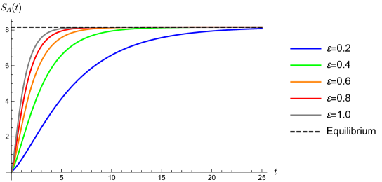
One also depicts a generic behaviour of the entropy, which has been observed for various systems prepared in a state with initially
low entanglement entropy, : after some short transient period of time, which depends on
the initial state of the system, the entanglement entropy goes through a phase of linear or almost linear growth, , until it settles at the saturation phase. This kind of behaviour is observed
in the time evolution of various quantum systems that bear the signatures of quantum chaos [37, 38, 39, 40], or in the study of thermalization in some holographic systems [41, 42, 43, 44]. In particular,
the rate of growth of the entanglement entropy
in the phase of linear growth is connected to the scrambling time in chaotic quantum systems, or the Kolmogorov-Sinai entropy rate [45], in cases where the quantum system has a classical counterpart.
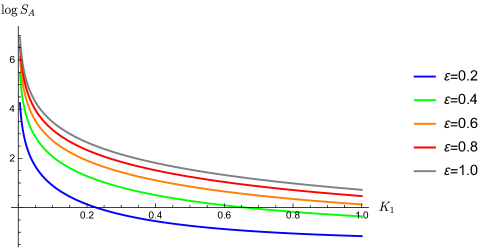
Finally, on figure 9 we show the logarithm of the entanglement entropy as a function of the scaled inverse temperature parameter at fixed finite moment of time . As expected the entropy decreases with increasing .
5.2 Entanglement entropy production rate
We calculate and analyse the entanglement production during the evolution of a
quantum mechanical dissipative system. Although entanglement entropy plays essential role in the thermalization of isolated quantum systems [46, 47, 48], the central quantity in non-equilibrium systems is not the entropy, but the rate of change of entropy, which is known as entropy production [49]. It serves as a measure of the irreversibility of a physical process.
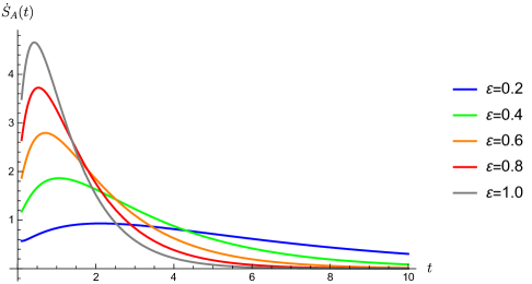
One can obtain the TFD entanglement entropy production rate (EEPR) by taking the time derivative of the extended non-equilibrium EE (5.6):
| (5.13) |
where the dot denotes derivative with respect to time . The entanglement entropy production rate is shown on figure 10 for several values of the dissipation parameter . One notices that for short time the EEPR reaches peak value, after which it monotonously decreases with time. The local maximum of agrees with the Zeigler’s principle of maximum entropy production [50, 51, 52]. Furthermore the EEPR is positive quantity which is expected and confirms the statement of the second law of thermodynamics for non-equilibrium systems. One also notes that the peak entropy production is bigger for strongly dissipative systems (large values of ).
6 Conclusion
In this paper we study the extended entanglement entropy of non-trivial quantized system, namely the closed bosonic string in a homogeneous plane wave geometry.
The EREE dependence on the inverse scaled temperatures in the ground state of the string has been explicitly shown analytically and graphically in four and five dimensions. The parameter space in these cases is one- and two-dimensional manifold correspondingly. The result shows that EREE increases with increasing temperature, while at very high temperatures (zero inverse scaled temperatures) the entropy diverges. This is also true for the components of the Fisher metric, which is an indication of an instability of the system or a phase transition. To address this problem we have analysed analytically the singularities in the scalar curvature of the metric. We have shown that the Ricci scalar is regular everywhere, including at very high temperatures. This suggests that the considered bosonic string system does not possess any critical points, representing a second-order phase transition, although a first order phase transition is not excluded at high temperature.
The graphical and analytical study of the scalar curvature showed that there are three geometrically different regions, corresponding to different types of interactions. Near the origin (fig. 5) the scalar curvature is non-zero and positive, thus defining elliptical geometry on the statistical manifold of thermodynamic parameters. In this case the absolute value of the local maximum of the curvature corresponds to the strongest interaction in the quasi-system. For lower temperatures (fig. 7) the curvature becomes negative, thus defining a hyperbolic geometry. Here, the strongest interaction is given by the absolute value of the local minimum of the curvature. The value of the scalar curvature on the level curve (fig. 6), which separates the different geometric regions, is zero, thus corresponding to a free, non-interacting theory. The limit value of the Ricci scalar at the origin (high temperatures) and at infinity (low temperatures) is also zero, which again leads to a free theory in these cases.
In the one-parameter case the Fisher distance has been derived, which is a measure of dissimilarity between two probability distribution functions. We have shown graphically that in this case the Fisher distance increases monotonously for increasing values of the upper limit of the defining integral. This is interpreted by the theory of fluctuations due to Ruppeiner [22] in the following manner: the probability of a fluctuation between two equilibrium string states decreases with the increasing of the distance between them.
We have also shown that the general expressions for the entanglement entropy (2.18) and the Fisher information matrix (2.19) work also for other quantum models. Some particular examples were considered, namely BCS-type bosonic systems and XY model in a magnetic field, which is a generalization of the Ising model.
We also manage to derive explicit expression for the entanglement entropy in the non-equilibrium case for a system with dissipation. We showed that the time-dependent entropy increases with time, until it settles at equilibrium (thermalization of the system). The equilibrium value of the entanglement entropy coincides with the thermal equilibrium entanglement entropy derived for a time-independent system. This is also in agreement with the second law of thermodynamics.
We also depicted one generic behaviour of the entanglement entropy, namely after a transient time which depends on the details of
the initial state of the system, the entanglement entropy goes through a phase of linear or almost linear growth, , until it settles at the saturation phase. It is also interesting to point out that this kind of behaviour of the entanglement entropy is observed
in the time evolution of various quantum systems that signify quantum chaos [37, 38, 39, 40], or in the study of thermalization in some holographic systems [41, 42, 43, 44].
The entropy increase rate have also been studied for several values of the dissipation parameter . We have shown that shortly after the initial moment the entanglement entropy production rate reaches peak value, after which it monotonously decreases with time. The local maximum of confirms the Zeigler’s principle of maximum entropy production [50, 51, 52]. Furthermore the EEPR is positive quantity which is just the statement of the second law of thermodynamics.
Another interesting question is how to reconstruct a parametric family of probability distributions corresponding to the given Fisher metric and to define under what conditions such reconstruction is possible. The Fisher information metric can be straightforwardly calculated once a probability distribution has been chosen. A set of distributions , parametrized by , forms a statistical manifold. The Riemannian metric on this manifold is the Fisher information metric defined by the following Lebesgue integral:
| (6.1) |
Here is a point from the sample space . It can be proved that the only
Riemannian metric is Fisher metric for which the geometry is invariant
under coordinate transformations of and also under
one-to-one transformations of random variable [30, 31]. The Fisher metric is also a solution to the Einstein field equations, which can be useful in finding the corresponding family of probability distributions . Unfortunately the equations are highly non-linear and cumbersome. The defining integral (6.1) only imposes non-trivial constraints on the probability distribution.
Although this survey is instigated more or less by the fact that
superstring theory on pp-wave backgrounds is exactly solvable, the TFD
framework is powerful enough to treat more complicated supergravity
background solutions. Extending the scope of the present research, next
natural step is to initiate a more thorough investigation of the
geometric, thermodynamic and information-theoretic aspects of some certain
holographic models. Such models, for instance, are the and Pilch-Warner solutions [53, 54, 55], Lunin-Maldacena background [56], some recent non-abelian T-dual solutions [57, 58, 59, 60, 61, 62] and their Penrose-Gven limit [63, 64] or pp-wave limit [65, 66, 62], the latter being easier to study with the techniques used in this paper. Such investigations are expected to shed light on the interplay between
spacetime, global and local properties in holography.
Acknowledgements
The authors would like to thank D. Marvakov for the fruitful discussions. This work was partially supported by the Bulgarian NSF grant T02/6 and Sofia University Research Fund grants № 80-10-116, № 80-10-118 and № 80-10-148.
References
- [1] S. Ryu and T. Takayanagi, “Holographic derivation of entanglement entropy from AdS/CFT,” Phys. Rev. Lett. 96 (2006) 181602, arXiv:hep-th/0603001 [hep-th].
- [2] T. Nishioka, S. Ryu, and T. Takayanagi, “Holographic Entanglement Entropy: An Overview,” J. Phys. A42 (2009) 504008, arXiv:0905.0932 [hep-th].
- [3] M. Van Raamsdonk, “Building up spacetime with quantum entanglement,” Gen. Rel. Grav. 42 (2010) 2323–2329, arXiv:1005.3035 [hep-th]. [Int. J. Mod. Phys.D19,2429(2010)].
- [4] M. Rangamani and T. Takayanagi, “Holographic Entanglement Entropy,” arXiv:1609.01287 [hep-th].
- [5] E. P. Verlinde, “Emergent Gravity and the Dark Universe,” arXiv:1611.02269 [hep-th].
- [6] Y. Takahashi and H. Umezawa, “Collective phenomena,” Int. J. Mod. Phys. 2 (1975) 55–57.
- [7] Y. TAKAHASHI and H. UMEZAWA, “Thermo field dynamics,” International Journal of Modern Physics B 10 no. 13n14, (1996) 1755–1805.
- [8] U. Fano, “Description of states in quantum mechanics by density matrix and operator techniques,” Rev. Mod. Phys. 29 (Jan, 1957) 74–93.
- [9] I. Prigogine, A Unified Formulation of Dynamics and Thermodynamics: With Special Reference to Non Equilibrium Statistical Thermodynamics. NORDITA publications: Nordisk Institut for Teoretisk Atomfysik. Nordisk Institut for teoretisk Atomfysik, 1972.
- [10] T. Arimitsu and H. Umezawa, “Nonequilibrium Thermo Field Dynamics,” Prog. Theor. Phys. 77 (1987) 32.
- [11] M. Suzuki, “Thermo field dynamics in equilibrium and non-equilibrium interacting quantum systems,” Journal of the Physical Society of Japan 54 no. 12, (1985) 4483–4485.
- [12] N. N. Bogolyubov, “A New method in the theory of superconductivity. I,” Sov. Phys. JETP 7 (1958) 41–46. [Front. Phys.6,399(1961)].
- [13] M.-w. Xiao, “Theory of transformation for the diagonalization of quadratic Hamiltonians,” ArXiv e-prints (Aug., 2009) , arXiv:0908.0787 [math-ph].
- [14] K. Nakagawa, “Entanglement entropies of coupled harmonic oscillators,” arXiv:1601.03584 [cond-mat.stat-mech].
- [15] “Diagonalization of bosonic quadratic hamiltonians by bogoliubov transformations,” Journal of Functional Analysis 270 no. 11, (2016) 4340 – 4368.
- [16] J. Dereziński, “Bosonic quadratic Hamiltonians,” ArXiv e-prints (Aug., 2016) , arXiv:1608.03289 [math-ph].
- [17] Y. Hashizume and M. Suzuki, “Understanding quantum entanglement by thermo field dynamics,” Physica A: Statistical Mechanics and its Applications 392 no. 17, (2013) 3518 – 3530.
- [18] K. Nakagawa, “Entanglement Entropies of Non-Equilibrium Finite-Spin Systems,” ArXiv e-prints (Oct., 2014) , arXiv:1410.6988 [cond-mat.stat-mech].
- [19] H. Dimov, S. Mladenov, R. C. Rashkov, and T. Vetsov, “Entanglement of higher-derivative oscillators in holographic systems,” Nucl. Phys. B918 (2017) 317–336, arXiv:1607.07807 [hep-th].
- [20] H. Matsueda, “Geometry and Dynamics of Emergent Spacetime from Entanglement Spectrum,” arXiv:1408.5589 [hep-th].
- [21] H. Matsueda, “Geodesic Distance in Fisher Information Space and Holographic Entropy Formula,” arXiv:1408.6633 [hep-th].
- [22] G. Ruppeiner, “Riemannian geometry in thermodynamic fluctuation theory,” Rev. Mod. Phys. 67 (Jul, 1995) 605–659.
- [23] H. Dimov, S. Mladenov, R. C. Rashkov, and T. Vetsov, “Thermo-field dynamics of higher-derivative oscillators,” Bulgarian Journal of Physics 44 no. 1, (2017) .
- [24] J. Bardeen, L. N. Cooper, and J. R. Schrieffer, “Theory of superconductivity,” Phys. Rev. 108 (Dec, 1957) 1175–1204.
- [25] O. Har-Shemesh, R. Quax, A. G. Hoekstra, and P. M. A. Sloot, “Information geometric analysis of phase transitions in complex patterns: the case of the Gray-Scott reaction-diffusion model,” Journal of Statistical Mechanics: Theory and Experiment 4 (Apr., 2016) 043301, arXiv:1512.02077 [cond-mat.stat-mech].
- [26] S. I. R. Costa, S. A. Santos, and J. E. Strapasson, “Fisher information distance: a geometrical reading,” ArXiv e-prints (Oct., 2012) , arXiv:1210.2354 [stat.ME].
- [27] J. Alvarez-Jimenez, A. Dector, and J. D. Vergara, “Quantum Information Metric and Berry Curvature from a Lagrangian Approach,” JHEP 03 (2017) 044, arXiv:1702.00058 [hep-th].
- [28] M. Blau, M. O’Loughlin, G. Papadopoulos, and A. A. Tseytlin, “Solvable models of strings in homogeneous plane wave backgrounds,” Nucl. Phys. B673 (2003) 57–97, arXiv:hep-th/0304198 [hep-th].
- [29] J. Burbea and C. R. Rao, “Differential metrics in probability spaces,” Probab.Math.Statist. 3 no. 2, (1984) 241–258.
- [30] S. Amari and H. Nagaoka, Methods of Information Geometry. Translations of mathematical monographs. American Mathematical Society, 2007.
- [31] S. Amari, Information Geometry and Its Applications. Applied Mathematical Sciences. Springer Japan, 2016.
- [32] D. C. Brody and A. Ritz, “Geometric Phase Transitions,” eprint arXiv:cond-mat/9903168 (Mar., 1999) , cond-mat/9903168.
- [33] D. C. Brody and A. Ritz, “Information geometry of finite ising models,” Journal of Geometry and Physics 47 no. 2–3, (2003) 207 – 220.
- [34] D. C. Brody and D. W. Hook, “Information geometry in vapour–liquid equilibrium,” Journal of Physics A: Mathematical and Theoretical 42 no. 2, (2009) 023001.
- [35] P. Kumar, S. Mahapatra, P. Phukon, and T. Sarkar, “Geodesics in information geometry: Classical and quantum phase transitions,” Phys. Rev. E 86 (Nov, 2012) 051117.
- [36] R. Maity, S. Mahapatra, and T. Sarkar, “Information geometry and the renormalization group,” Phys. Rev. E 92 (Nov, 2015) 052101.
- [37] W. H. Zurek and J. P. Paz, “Decoherence, chaos, and the second law,” Phys. Rev. Lett. 72 (1994) 2508, arXiv:gr-qc/9402006 [gr-qc].
- [38] A. K. Pattanayak, “Lyapunov exponents, entropy production and decoherence,” in eprint arXiv:chao-dyn/9911017. 1999.
- [39] D. Monteoliva and J. P. Paz, “Decoherence and the Rate of Entropy Production in Chaotic Quantum Systems,” Physical Review Letters 85 (Oct., 2000) 3373–3376, quant-ph/0007052.
- [40] A. Tanaka, H. Fujisaki, and T. Miyadera, “Saturation of the production of quantum entanglement between weakly coupled mapping systems in a strongly chaotic region,” Phys. Rev. E 66 no. 4, (Oct., 2002) 045201, quant-ph/0209086.
- [41] V. Balasubramanian, A. Bernamonti, J. de Boer, N. Copland, B. Craps, E. Keski-Vakkuri, B. Muller, A. Schafer, M. Shigemori, and W. Staessens, “Thermalization of Strongly Coupled Field Theories,” Phys. Rev. Lett. 106 (2011) 191601, arXiv:1012.4753 [hep-th].
- [42] V. Balasubramanian, A. Bernamonti, J. de Boer, N. Copland, B. Craps, E. Keski-Vakkuri, B. Muller, A. Schafer, M. Shigemori, and W. Staessens, “Holographic Thermalization,” Phys. Rev. D84 (2011) 026010, arXiv:1103.2683 [hep-th].
- [43] T. Hartman and J. Maldacena, “Time Evolution of Entanglement Entropy from Black Hole Interiors,” JHEP 05 (2013) 014, arXiv:1303.1080 [hep-th].
- [44] H. Liu and S. J. Suh, “Entanglement growth during thermalization in holographic systems,” Phys. Rev. D89 no. 6, (2014) 066012, arXiv:1311.1200 [hep-th].
- [45] E. Bianchi, L. Hackl, and N. Yokomizo, “Linear growth of the entanglement entropy and the Kolmogorov-Sinai rate,” arXiv:1709.00427 [hep-th].
- [46] A. Polkovnikov, K. Sengupta, A. Silva, and M. Vengalattore, “Colloquium: Nonequilibrium dynamics of closed interacting quantum systems,” Reviews of Modern Physics 83 no. 3, (2011) 863, arXiv:1007.5331 [cond-mat.stat-mech].
- [47] C. Gogolin and J. Eisert, “ Equilibration, thermalisation, and the emergence of statistical mechanics in closed quantum systems,” Rep.Prog.Phys. 79 no. 5, (2016) , arXiv:1503.07538 [quant-ph].
- [48] L. D’Alessio, Y. Kafr, A. Polkovnikov, and M. Rigol, “ From quantum chaos and eigenstate thermalization to statistical mechanics and thermodynamics,” Advances in Physics 65 no. 3, (2016) , arXiv:1509.06411 [cond-mat.stat-mech].
- [49] S. R. De Groot and P. Mazur, Non-equilibrium thermodynamics. Dover Publications Inc., 1984.
- [50] Z. H. S. I. N. Naghdi, P. M. and R. Hill, Progress in solid mechanics: Volume IV. Amsterdam: North-Holland, 1963.
- [51] H. Ziegler, An Introduction to Thermomechanics. North-Holland: Amsterdam, The Netherlands, 1983.
- [52] H. Ziegler and C. Wehrli, “On a Principle of Maximal Rate of Entropy Production,” Journal of Non-Equilibrium Thermodynamics 12 no. 3, (2009) .
- [53] K. Pilch and N. P. Warner, “A New supersymmetric compactification of chiral IIB supergravity,” Phys. Lett. B487 (2000) 22–29, arXiv:hep-th/0002192 [hep-th].
- [54] K. Pilch and N. P. Warner, “ supersymmetric renormalization group flows from IIB supergravity,” Adv. Theor. Math. Phys. 4 (2002) 627–677, arXiv:hep-th/0006066 [hep-th].
- [55] K. Pilch and N. P. Warner, “ supersymmetric RG flows and the IIB dilaton,” Nucl. Phys. B594 (2001) 209–228, arXiv:hep-th/0004063 [hep-th].
- [56] O. Lunin and J. M. Maldacena, “Deforming field theories with global symmetry and their gravity duals,” JHEP 05 (2005) 033, arXiv:hep-th/0502086 [hep-th].
- [57] K. Sfetsos and D. C. Thompson, “On non-abelian T-dual geometries with Ramond fluxes,” Nucl. Phys. B846 (2011) 21–42, arXiv:1012.1320 [hep-th].
- [58] G. Itsios, Y. Lozano, E. O Colgain, and K. Sfetsos, “Non-Abelian T-duality and consistent truncations in type-II supergravity,” JHEP 08 (2012) 132, arXiv:1205.2274 [hep-th].
- [59] z. Kelekci, Y. Lozano, N. T. Macpherson, and E. . Colgáin, “Supersymmetry and non-Abelian T-duality in type II supergravity,” Class. Quant. Grav. 32 no. 3, (2015) 035014, arXiv:1409.7406 [hep-th].
- [60] Y. Lozano, E. O Colgain, K. Sfetsos, and D. C. Thompson, “Non-abelian T-duality, Ramond Fields and Coset Geometries,” JHEP 06 (2011) 106, arXiv:1104.5196 [hep-th].
- [61] N. T. Macpherson, C. Nunez, D. C. Thompson, and S. Zacarias, “Holographic Flows in non-Abelian T-dual Geometries,” JHEP 11 (2015) 212, arXiv:1509.04286 [hep-th].
- [62] H. Dimov, S. Mladenov, R. C. Rashkov, and T. Vetsov, “Non-abelian T-duality of Pilch-Warner background,” Fortsch. Phys. 64 (2016) 657–673, arXiv:1511.00269 [hep-th].
- [63] R. Penrose, Any Space-Time has a Plane Wave as a Limit, pp. 271–275. Springer Netherlands, Dordrecht, 1976.
- [64] R. Gueven, “Plane wave limits and T-duality,” Phys. Lett. B482 (2000) 255–263, arXiv:hep-th/0005061 [hep-th].
- [65] R. Corrado, N. Halmagyi, K. D. Kennaway, and N. P. Warner, “Penrose limits of RG fixed points and PP waves with background fluxes,” Adv. Theor. Math. Phys. 6 (2003) 597–617, arXiv:hep-th/0205314 [hep-th].
- [66] D. Brecher, C. V. Johnson, K. J. Lovis, and R. C. Myers, “Penrose limits, deformed pp waves and the string duals of large gauge theory,” JHEP 10 (2002) 008, arXiv:hep-th/0206045 [hep-th].