Cross-Layer Optimization of Wireless Links
under Reliability and Energy Constraints

Abstract

The vision of connecting billions of battery operated devices to be used for diverse emerging applications calls for a wireless communication system that can support stringent reliability and latency requirements. Both reliability and energy efficiency are critical for many of these applications that involve communication with short packets which undermine the coding gain achievable from large packets. In this paper, we study a cross-layer approach to optimize the performance of low-power wireless links. At first, we derive a simple and accurate packet error rate (PER) expression for uncoded schemes in block fading channels based on a new proposition that shows that the waterfall threshold in the PER upper bound in Nakagami-$m$ fading channels is tightly approximated by the $m$-th moment of an asymptotic distribution of PER in AWGN channel. The proposed PER approximation establishes an explicit connection between the physical and link layers parameters, and the packet error rate. We exploit this connection for cross-layer design and optimization of communication links. To this end, we propose a semi-analytic framework to jointly optimize signal-to-noise ratio (SNR) and modulation order at physical layer, and the packet length and number of retransmissions at link layer with respect to distance under the prescribed delay and reliability constraints.

I Introduction

The upcoming wireless networks are required to support massive number of devices under the umbrella of internet-of-things (IoT). The heterogeneity of use cases of these machine-to-machine (M2M) type communication necessitate diverse reliability and latency requirements. As the devices will be mostly battery operated, energy efficiency also becomes a critical issue. Moreover, this novel traffic type uses short packets which undermine the coding gain achievable from large packets [1][2]. All these factors urge a new look not only into physical layer but also cross-layer design in order to ensure reliability under energy constraints. In this paper, we improve the packet error rate (PER) approximations over block-fading channels in order to have a better control over the parameters that determine the system performance and utilize these insights to optimize cross-layer parameters, e.g., packet length, number of retransmission, modulation scheme.

The average PER is an important metric for cross-layer optimization of wireless transmissions over block-fading channels. For instance, the objective function to optimize throughput, energy or spectral efficiency of a transmission scheme is defined in relation to the average PER [3][4], and the parameters maximizing the system performance are determined. However, the average PER, except for certain simple cases, is not found in exact closed form, although it can usually be written in the integral form. The integral then needs to be evaluated numerically and may not be computationally intensive, however this approach in general does not offer insights as to what parameters determine the system performance.

One such closed form is the upper bound on average PER for both the uncoded and coded schemes in Rayleigh fading, $1-\exp(\omega_{0}/\bar{\gamma})$, where $\bar{\gamma}$ is the average signal-to-noise ratio (SNR) and $\omega_{0}$ is the waterfall threshold [5]. The threshold is defined as an integral of the PER function in the AWGN channel. In [5], also a similar upper bound in Nakagami-$m$ fading is proposed with a corresponding threshold. In both cases, however, a closed-form solution to the threshold is not feasible. A log-domain linear approximation of $\omega_{0}$ is developed for uncoded schemes in [6], and for (un)coded schemes in [7]. However, the approximation in [6] is tight for large packets only while in [7] the approximation parameters for a given modulation scheme are calculated by simulations. For uncoded schemes, an accurate PER expression is derived in [8] that is complicated to utilize for link optimization.

In this paper, we show that the waterfall threshold in the PER upper bound under Nakagami-$m$ block fading is tightly approximated by the $m$-th moment of an asymptotic distribution of PER function in AWGN. In Rayleigh fading, the approximation leads to a PER approximation which is accurate than [6][7] and also maintains explicit connection with modulation order unlike [7].

Note that in today’s age of battery operated devices, the number one design goal is energy efficient communication. However, the emerging delay and reliability requirements have a direct impact on the needed energy to transfer each information bit. The reliability depends on the bit error or packet error statistics of the wireless channel, which in turn depend on the choice of the system parameters such as transmit power, modulation scheme, packet length etc. If the packet error probability has to be reduced so as to transfer a packet with limited number of retransmission, these parameters need to be optimized while keeping a tab on the energy consumption.

How to select the modulation order and transmission power to attain energy-efficient communication is studied in AWGN channel [9, 10, 11] and in fading channels [4][7]. These studies in general suggest using higher order modulations at smaller distances as opposed to the common notion followed in wireless sensor networks (WSN) by choosing low-order modulations for their low SNR requirement. For instance, low-power transceivers CC1100 and CC2420, often used in WSNs, employ BPSK and QPSK. In fading channels, it is shown in [4][7] that there exist an optimal SNR and packet length for each modulation scheme at which the required energy for successful transfer of an information bit is minimized. In [4], the optimal SNR is conditioned on the maximum transmit power however this constraint is ignored in [7]. In these studies, no restriction on number of retransmission is imposed and as a result the optimal SNR is not bound to satisfy the reliability target.

In this paper, we study the energy minimization in fading channels however under the often neglected reliability constraints. We exploit the proposed PER approximation for cross-layer optimization of a power-limited system in Rayleigh block-fading channels. By defining a energy consumption model for per payload bit transferred, we find the optimal (energy consumption minimizing) system parameters while maintaining the reliability and delay target. Specifically, i) for a system with fixed modulation scheme (e.g., CC2420) and report size, we propose closed-form conditions for energy optimal SNR that conform to the maximum transmit power and reliability constraints, ii) for a general power-limited system, we propose a joint optimization algorithm to find the physical layer (SNR, modulation order) and link layer (packet length, number of retransmissions) parameters with respect to distance under the prescribed delay and reliability constraints.

The rest of the paper is organized as follows. Section II develops an approximation to average PER in block fading channels. Section III defines the cross-layer optimization problem, solves it under the reliability constraints and presents the results. Section IV draws the concluding remarks.

II The Average PER in Block Fading

Let $f\left(\gamma\right)$ be the PER function in the AWGN channel with instantaneous SNR, $\gamma$. Then, for an $N$-bit uncoded packet with bit error rate (BER) function $b_{e}\left(\gamma\right)$, $f\left(\gamma\right)$ is defined as

$$\vspace{-2pt}f(\gamma)=1-\Big{(}1-b_{e}\left(\gamma\right)\Big{)}^{N}$$ (1)

Also, let $p\left(\gamma;\bar{\gamma}\right)$ be the probability distribution function (PDF) of the received instantaneous SNR. In Nakagami-$m$ fading, $\gamma$ follows the Gamma distribution with PDF

$$p(\gamma;\bar{\gamma})=\frac{m^{m}\gamma^{m-1}}{\bar{\gamma}^{m}\Gamma(m)}\mathrm{exp}\Big{(}-\frac{m\gamma}{\bar{\gamma}}\Big{)},\gamma\geq 0$$ (2)

The average PER, denoted as $\bar{P_{e}}\left(\bar{\gamma}\right)$, is then computed by integrating (1) over (2)

$$\bar{P_{e}}\left(\gamma\right)=\int_{0}^{\infty}f(\gamma){p(\gamma;\bar{\gamma})}d\gamma$$ (3)

In [5], it is shown that $\bar{P_{e}}\left(\bar{\gamma}\right)$ is upper bounded by

$$\bar{P_{e}}\left(\gamma\right)\leq\frac{m^{m-1}B}{\bar{\gamma}^{m-1}\Gamma\left(m\right)}\left(1-\mathrm{exp}\left(-\frac{m\omega_{m}}{\bar{\gamma}B}\right)\right)$$ (4)

where $0\leq\gamma^{m-1}f\left(\gamma\right)\leq B$ and $\omega_{m}$ is defined as,

$$\omega_{m}=\int_{0}^{\infty}{\gamma^{m-1}f\left(\gamma\right)d\gamma}$$ (5)

In Rayleigh fading (i.e., $m=1$), as $f\left(\gamma\right)$ is the probability we have $0\leq f\left(\gamma\right)\leq 1$, and (4) can be written as,

$$\bar{P_{e}}\left(\gamma\right)\leq 1-\mathrm{exp}\left(-\frac{\omega_{0}}{\bar{\gamma}}\right)$$ (6)

where $\omega_{0}$ from (5) becomes

$$\omega_{0}=\int_{0}^{\infty}{f\left(\gamma\right)d\gamma}$$ (7)

In what follows, we propose generic approximations to $\omega_{0}$ and $\omega_{m}$ for uncoded schemes with BER functions as

$$b_{e}(\gamma)=c_{m}\mathrm{exp}\left(-k_{m}\gamma\right)$$ (8)

$$b_{e}(\gamma)=c_{m}Q\left(\sqrt{k_{m}\gamma}\right)$$ (9)

where $c_{m}$ and $k_{m}$ are modulation-dependent constants. Non-coherent FSK and DPSK have the BER in the form of (8) while M-ASK, M-PAM, MSK, M-PSK and M-QAM have BER in the Gaussian $Q$-function form (9)[5].

II-A Approximations to $\omega_{0}$ and $\omega_{m}$

Proposition 1: For uncoded transmission of a packet with length $N$, with the BER functions described by $c_{m}e^{-k_{m}\gamma}$ and $c_{m}Q(\sqrt{k_{m}\gamma})$ where $0<c_{m}\leq 1$ and $k_{m}>0$, the threshold, $\omega_{m}$, in Nakagami-$m$ fading channel for integer values of the fading parameter is approximated by the mth moment of the Gumbel distribution for sample maximum

$$\omega_{m}\approx\frac{\mathbb{E}[\gamma^{m}]}{m}$$ (10)

Proof: For packet length $N$, the PER function in (1) for BER functions described by $c_{m}e^{-k_{m}\gamma}$ and $c_{m}Q(\sqrt{k_{m}\gamma})$ can be asymptotically approximated by the Gumbel distribution function for the sample minimum [8]

$$f(\gamma)\simeq 1-\mathrm{exp}\left(-\mathrm{exp}\left(-\frac{\gamma-a_{N}}{b_{N}}\right)\right)$$ (11)

where $a_{N}$ and $b_{N}>0$ are the normalizing constants.

Let $G\left(\gamma\right)=\mathrm{exp}(-\mathrm{exp}(-\frac{\gamma-a_{N}}{b_{N}}))$ be the cumulative distribution function (CDF) of the Gumbel distribution for the sample maximum, then from (11) and (5) we have

$$\omega_{m}\approx\int_{0}^{\infty}{\gamma^{m-1}\Big{(}1-G\left(\gamma\right)\Big{)}d\gamma}$$ (12)

Assuming $\gamma=y^{\frac{1}{m}}$ and $\gamma^{m-1}d\gamma={dy}/{m}$, from (12) we get

$$\omega_{m}\approx\frac{1}{m}\int_{0}^{\infty}{1-G\left(y^{\frac{1}{m}}\right)dy}$$ (13)

Let $g(\gamma)={dG(\gamma)}/{d\gamma}$ be the PDF, then with some manipulation and changing the order of integration in (13)

$$\omega_{m} \approx\frac{1}{m}\int_{0}^{\infty}{\int_{y^{\frac{1}{m}}}^{\infty}g\left(\gamma\right)d\gamma dy}$$

$$=\frac{1}{m}\int_{0}^{\infty}{\int_{0}^{\gamma^{m}}g\left(\gamma\right)dyd\gamma}$$

$$=\frac{1}{m}\int_{0}^{\infty}{\gamma^{m}g(\gamma)d\gamma}.$$ (14)

Noting that the integral in the last equality is the $m$th moment of a continuous and nonnegative random variable $\gamma$ with the PDF $g(\gamma)$ completes the proof. $\blacksquare$

One can find the mth moment of the Gumbel distribution from its moment generating function (MGF) defined as

$$M_{\gamma}\left(t\right)\triangleq\Gamma\Big{(}1-b_{N}\,t\Big{)}\,e^{{a_{N}\,t}}$$ (15)

where $\Gamma\left(\cdot\right)$ is the standard gamma function.

In Rayleigh fading with $m=1$, from (10) and (15), $\omega_{0}$ equals the expected value of the Gumbel distribution, i.e.

$$\omega_{0}\approx\mathbb{E}[\gamma]=a_{N}+\gamma_{e}\,b_{N}$$ (16)

where $\gamma_{e}=0.5772$ is the Euler constant. Notation $\omega_{0}$ is preferred over $\omega_{1}$ to remain consistent with the prior works. Similarly, for $m=2$ and $m=3$, which represent the next two significant fading conditions, (10) under (15) becomes

$$\begin{split}\omega_{2}\!\approx\!\frac{\mathbb{E}[\gamma^{2}]}{2}\!=&\frac{1}{2}\Big{[}a_{N}^{2}+1.64b_{N}^{2}+\gamma_{e}^{2}b_{N}^{2}+2\gamma_{e}a_{N}b_{N}\Big{]}\end{split}$$ (17)

$$\begin{split}\omega_{3}\!\approx\!\frac{\mathbb{E}[\gamma^{3}]}{3}\!=&\frac{1}{3}\Big{[}4.93\gamma_{e}b_{N}^{3}\!+\!4.93a_{N}b_{N}^{2}\!+\!a_{N}^{3}\!+\!2.40b_{N}^{3}\\ &\quad\,\,\,+\gamma_{e}^{3}b_{N}^{3}+3\gamma_{e}^{2}a_{N}b_{N}^{2}+3\gamma_{e}a_{N}^{2}b_{N}\Big{]}\end{split}$$ (18)

The normalizing constants for BER function in (8) are [8]

$$a_{N}=\frac{\log(Nc_{m})}{k_{m}},\,\,\,\,\,\,\,\,b_{N}=\frac{1}{k_{m}}$$ (19)

whereas the constants for BER in (9) are

$$a_{N} =\frac{2}{k_{m}}\Big{[}\mathrm{erf}^{-1}\Big{(}1-\frac{2}{Nc_{m}}\Big{)}\Big{]}^{2}$$ (20)

$$b_{N} =\frac{2}{k_{m}}\Big{[}\mathrm{erf}^{-1}\Big{(}1-\frac{2}{Nc_{m}e}\Big{)}\Big{]}^{2}-a_{N}$$

where $e$ is the base of the natural logarithm.

II-B The Average PER with New Parametrization

Using the normalizing constants (19) in (10), the average PER in (4) and (6) can be expressed in the form of elementary functions. However due to the inverse error function in (20), (4) and (6) cannot be simplified further. An intuitive approach is to utilize an exponential function based approximation of $Q$-function (e.g., [12]), and utilize $a_{N}$ and $b_{N}$ from (19). However, this approach loses the approximation accuracy. Instead, our objective is to find the exponential function approximation for given $a_{N}$ and $b_{N}$ in (19) and $\omega_{m}$ approximation in (10) that fits best to the integral expression in (5) or (7). In essence, we reformulate $a_{N}$ and $b_{N}$ in (19) as

$$a_{N}\approx\frac{\log(k_{1}Nc_{m})}{k_{2}k_{m}},\,\,\,\,\,\,\,\,b_{N}\approx\frac{1}{k_{2}k_{m}}$$ (21)

and find the constants $k_{1}$ and $k_{2}$. We estimated $k_{1}$ and $k_{2}$ for BPSK modulation by numerically evaluating (7) and matching it with (16) under $a_{N}$ and $b_{N}$ in (21). For a packet length $N$ in an interval $[32,1024]$ bits, the optimal constants are: $k_{1}=0.2114$ and $k_{2}=0.5598$. We find that these constants are independent of modulation schemes with the BER function involving $Q$-function. As a result, a simple PER approximation can also be reached for the modulation schemes with the BER function $c_{m}Q(\sqrt{k_{m}\gamma})$. For instance, let $\acute{c}_{m}=k_{1}c_{m}$ and $\acute{k}_{m}=k_{2}k_{m}$, then from (21) and (16), the PER in Rayleigh fading is

$$\bar{P}_{e}(\bar{\gamma})\approx 1-\left(N\acute{c}_{m}\right)^{-\frac{1}{\acute{k}_{m}\bar{\gamma}}}\mathrm{exp}\left(-\frac{\gamma_{e}}{\acute{k}_{m}\bar{\gamma}}\right).$$ (22)

where $\acute{c}_{m}=c_{m}$ and $\acute{k}_{m}=k_{m}$ for the BER function $c_{m}e^{-k_{m}\gamma}$.

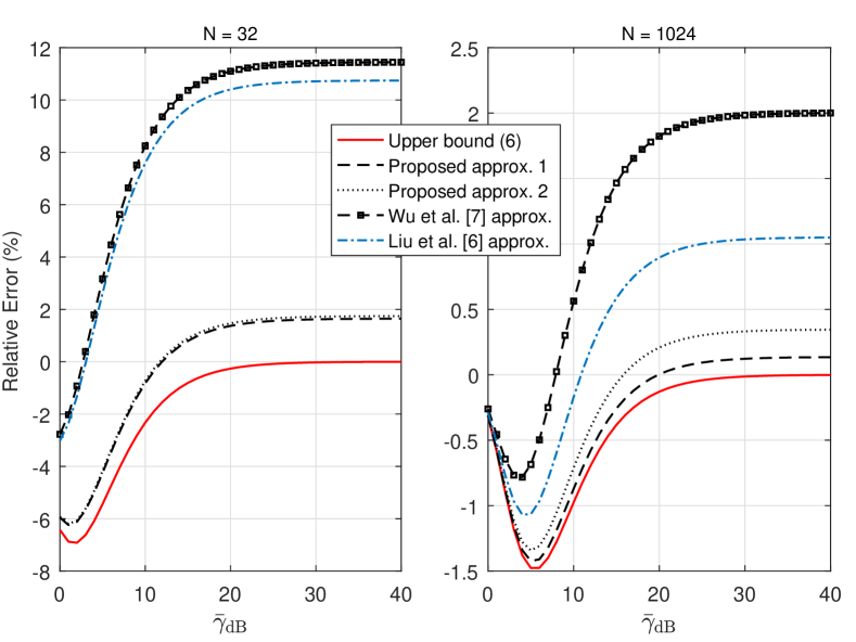
(a) 4 QAM

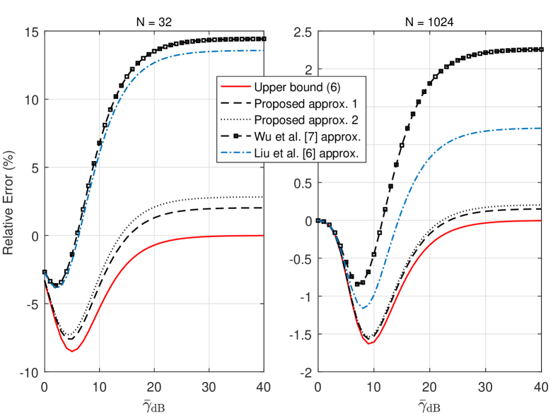
(b) 16 QAM

Figure 1: Relative error in average PER in Rayleigh fading. Approx. 1 uses $a_{N}$ and $b_{N}$ from (20) while Approx. 2 is based on (21).

We evaluate the average PER in (4) with the proposed $\omega_{m}$ approximation in (10) with the original (20) and modified (21) parameters and validate it against the numerical evaluation of PER in (3). The approximations to (4) for Rayliegh fading channel proposed in [6][7] are also analyzed. Fig. 1(a) and Fig. 1(b) show the relative error (RE) in the proposed approximation and the reference studies for 4-QAM and 16-QAM in Rayleigh fading. Similar results (not shown here) are obtained for 64-QAM. It can be observed that the RE in average PER with $\omega_{0}$ approximations (20) and (21) are quite close to the upper bound (6), which is evaluated numerically, for small to large packet lengths. In comprison, the RE of approximations in [6][7] is small at low SNR, however it increases rapidly especially for small packet lengths. We also evaluated the average PER based on $\omega_{m}$ approximations in (17) and (18) and observed the similar accuracy.

III Energy Efficient Link Optimization

III-A Energy Consumption Model

We consider minimizing energy consumption of a wireless link between a transmitter and receiver pair separated by distance $d$. The energy consumption of the signal path at the transmitter and receiver is comprised of baseband processing blocks (e.g., (de)coding and (de)modulation) and radio-frequency (RF) chain that consists of a power amplifier (PA) and other electronic components such as analog-to-digital and digital-to-analog (AD/DA) converter, low-noise amplifier (LNA), filters, mixers and frequency synthesizers. However for an energy-constrained wireless system (e.g., WSN), the energy consumption of RF chain is orders of magnitude larger than that of baseband processing components. The power consumption of PA is considered to be proportional of the transmit power $P_{t}$ such that $P_{\mathrm{PA}}=\frac{\xi}{\eta}P_{t}$, where $\eta$ is the drain efficiency of the power amplifier (PA) and $\xi$ is the peak-to-average-power-ratio (PAPR). The PAPR depends on the modulation scheme and the associated constellation size. If baseband power consumption is neglected and the power consumption of all the other components in RF chain excluding PA is denoted as $P_{c}$, a simple power consumption model is $P_{\mathrm{on}}=\frac{\xi}{\eta}P_{t}+P_{c}$. From [9], this model leads to the total energy consumption to transmit and receive a symbol as

$$E_{\mathrm{sym}}=\frac{\xi}{\eta}E_{t}+\frac{P_{c}}{R_{s}}$$ (23)

where $E_{t}$ is the average transmission energy of a symbol and $R_{s}$ the physical layer symbol rate. For FSK, BPSK and QPSK modulations $\xi=1$ , for OQPSK $\xi=2.138$, and for a square MQAM modulation $\xi=3(\sqrt{M}-\frac{1}{\sqrt{M}}+1)$ [9].

Let $E_{b}={E_{r}}/{\log_{2}M}$ be the average received energy per uncoded bit where $E_{r}$ is the average received energy per symbol and $M$ is the constellation size, then the average SNR, $\bar{\gamma}$, at the receiver is

$$\bar{\gamma}=\frac{E_{r}}{N_{0}\log_{2}M}$$ (24)

Assuming a $\kappa$th-power path-loss model, the transmission energy at distance $d$ from (24) is expressed as [9]

$$E_{t}\triangleq E_{r}G_{d}=\Big{(}\bar{\gamma}N_{0}\log_{2}M\Big{)}G_{d}$$ (25)

where $G_{d}\triangleq G_{1}d^{\kappa}M_{\ell}$ is the pathloss gain with $G_{1}$, the gain factor at unit distance, depends on the transmit and receive antenna gains and carrier frequency, and $M_{l}$ the link margin.

In packet based wireless systems, the information bits are encapsulated into packets each carrying $n_{p}$ payload and $n_{h}$ overhead bits. The number of symbols in a packet are $n_{s}=(n_{h}+n_{p})/\log_{2}M$. The average energy required to transmit and receive an information bit per packet transmission, from (23) and (25), is

$$E_{\mathrm{0}}=\frac{n_{s}}{n_{p}}E_{\mathrm{sym}}=\frac{n_{p}+n_{h}}{n_{p}}A\bar{\gamma}+B$$ (26)

where $A={\xi N_{0}G_{d}}/{\eta}$ and $B=\frac{n_{s}}{n_{p}}\cdot\frac{P_{c}}{R_{s}}=\frac{P_{c}}{R_{b}}$ with $R_{b}=W\log_{2}M$ the physical layer bit rate in bandwidth $W$.

The total energy consumption of a wireless link depends on the required retransmissions before a packet is decoded successfully at the receiver. The retransmission statistics are determined by the PER, $P_{e}\left(\bar{\gamma}\right)$, which is a function of $\bar{\gamma}$, channel fading, and other parameters as discussed earlier. The number of retransmissions $\tau$ is geometric random variable and over an uncorrelated channel between retransmissions the average number of retransmissions are $\bar{\tau}={1}/{(1-\bar{P}_{e}(\bar{\gamma}))}$. Therefore, the total average energy for a successful transmission of a bit is $E=\bar{\tau}E_{0}$, which from (26) is

$$E=\frac{1}{1-\bar{P}_{e}(\bar{\gamma})}\left(\frac{n_{p}+n_{h}}{n_{p}}A\bar{\gamma}+B\right)$$ (27)

In formulating (27), no limit on the number of retransmissions is assumed. However for a delay constrained system, a packet must be delivered within maximum number of retransmissions $\tau_{r}^{\max}$ and the packet error probability after $\tau_{r}^{\max}$ retransmissions must be less than a reliability target $\varepsilon$

$$\left[\bar{P}_{e}(\bar{\gamma})\right]^{\tau_{r}^{\max}+1}\leq\varepsilon$$ (28)

From (28), the required PER $\varepsilon_{\mathrm{req}}$ to satisfy target $\varepsilon$ is

$$\bar{P}_{e}(\bar{\gamma})\leq\varepsilon^{1/(\tau_{r}^{\max}+1)}:=\varepsilon_{\mathrm{req}}$$ (29)

If (29) is satisfied, the average number of transmissions per packet is $\bar{\tau}_{\mathrm{trunc}}={1-[\bar{P}_{e}(\bar{\gamma})]^{\tau_{r}^{\max}+1}}/{(1-\bar{P}_{e}(\bar{\gamma}))}$ and the total average energy is given by

$$E_{\mathrm{trunc}}=\frac{1-[\bar{P}_{e}(\bar{\gamma})]^{\tau_{r}^{\max}+1}}{1-\bar{P}_{e}(\bar{\gamma})}\left(\frac{n_{p}+n_{h}}{n_{p}}A\bar{\gamma}+B\right)$$ (30)

In next section, we consider minimizing energy consumption per information bit in (27) while maintaining the PER constraint in (29).

III-B Link Optimization with Minimum Energy Consumption

III-B1 Optimal Average SNR

With $n_{p}$ fixed, finding the optimal average SNR represents a case where the sensors have to send a fixed size reports. The unconstrained energy minimization problem for optimal $\bar{\gamma}$ is modeled as

$$\underset{\bar{\gamma}}{\text{minimize}} E(\bar{\gamma})$$ (31)

subject to $$\bar{\gamma}\in\left[0,\infty\right]$$

The function $E$ is a product of two functions: $\bar{\tau}(\gamma)-$ the number of retransmissions with $\bar{\tau}^{{}^{\prime}}(\gamma)\leq 0$, and $E_{0}(\gamma)-$ the average energy per transmission attempt such that $E_{0}^{{}^{\prime}}(\gamma)\geq 0$ where $\acute{x}$ denotes the first derivative. If both $\bar{\tau}(\gamma)$ and $E_{0}(\gamma)$ are convex, then $E$ is also convex [7, Lemma 1] and the optimal $\bar{\gamma}$ can be obtained by solving $\frac{\partial E}{\partial\bar{\gamma}}=0$ which yields a quadratic equation with a positive root as

$$\bar{\gamma}^{*}=\frac{\omega_{0}}{2}+\sqrt{\omega_{0}\left(\frac{\omega_{0}}{4}+\frac{B}{A}\frac{n_{p}}{n_{h}+n_{p}}\right)}$$ (32)

Under the constraints on required PER and the transmit power, the minimization of energy in (27) can be written as

$$\underset{\bar{\gamma}}{\text{minimize}} E(\bar{\gamma})$$ (33)

subject to $$\bar{\gamma}_{\min}\leq\bar{\gamma}\leq\bar{\gamma}_{\max}$$

The minimum average SNR $\bar{\gamma}_{\min}$ requirement is set by the PER bound in (29), which can be obtained from (22)

$$\bar{\gamma}_{\min}=-\frac{\gamma_{e}+\log\Big{(}\acute{c}_{m}\left(n_{h}+n_{p}\right)\Big{)}}{\acute{k}_{m}\log\left(1-\varepsilon_{\mathrm{req}}\right)}$$ (34)

Due to the hardware and regulatory constraints, the transmission power cannot exceed a limit $P_{0}$. The condition $P_{\mathrm{tx}}\leq P_{0}$ translates to $\bar{\gamma}\leq\bar{\gamma}_{\max}$ with $\bar{\gamma}_{\max}$ from (25) is

$$\bar{\gamma}_{\max}=\frac{P_{0}}{WN_{0}G_{d}\log_{2}M}$$ (35)

From (34) and (35), the required SNR, denoted as $\bar{\gamma}^{*}_{\mathrm{req}}$, relates to the SNR for unconstrained case in (31) as

$$\bar{\gamma}_{\mathrm{req}}=\begin{dcases}\bar{\gamma}_{\min},&\bar{\gamma}^{*}<\bar{\gamma}_{\min}\\ \bar{\gamma}_{\max},&\bar{\gamma}^{*}>\bar{\gamma}_{\max}\\ \,\,\bar{\gamma}^{*},&\mathrm{otherwise}\\ \end{dcases}$$ (36)

which holds for $\bar{\gamma}_{\min}<\bar{\gamma}_{\max}$. If $\bar{\gamma}_{\min}>\bar{\gamma}_{\max}$, the reliability target cannot not be satisfied for a given modulation scheme.

III-B2 Optimal Payload Size

The function $E$ in (27) is also convex in payload size $n_{p}$ and its optimal value is

$$n_{p}^{*}=\!\!\frac{n_{h}\bar{\gamma}\left(\left(\acute{k}_{m}\!-1\right)\bar{\gamma}\!+\!\sqrt{\acute{k}_{m}^{2}\bar{\gamma}^{2}\!+\!2\acute{k}_{m}\bar{\gamma}\!+\!\frac{4Bk_{m}}{A}\!+\!1}\right)}{2\Big{(}\bar{\gamma}+\frac{B}{A}\Big{)}}$$ (37)

The upper limit on the payload size ${n_{p,\max}}$ is set by the minimum SNR requirement $\bar{\gamma}_{\min}$ to satisify PER target. It is given by from (29)

$${n_{p,\max}}=-n_{h}+\frac{10^{-(\gamma_{e}+\bar{\gamma}_{\min}\acute{k}_{m}\log\left(1-\varepsilon_{\mathrm{req}}\right))}}{\acute{c}_{m}}$$ (38)

where $\bar{\gamma}_{\min}$ is given in (34).

III-B3 Joint Optimal $\bar{\gamma},n_{p},M,\tau_{r}^{\max}$

As the IoT devices will be used in diverse scenarios, it might be important in many to find the optimal SNR, payload size, modulation order and number of retransmissions for energy efficient communication. For example after deployment in harsh and inaccessible areas, the devices will optimize those parameters for the first time and then can continue with the optimal setting. The joint optimization problem can be written as

$$\underset{\bar{\gamma},n_{p},M,\tau_{r}^{\max}}{\text{minimize}} E\Big{(}\bar{\gamma},n_{p},M,\tau_{r}^{\max}\Big{)}$$ (39)

where $M\in\{\mathrm{FSK,MPSK,MQAM}\}$ and $\tau_{r}^{\max}=i,\;i\geq 1$.

Note that these devices will support only few values of $M$ and a small value of $\tau_{r}^{\max}$ is feasible for minimum energy operation [7]. As a result, the exhaustive search over the combination of $M$ and $\tau_{r}^{\max}$ will not be computationally demanding. For each combination of $M$ and $\tau_{r}^{\max}$, the joint optimum $\bar{\gamma}$ and $n_{p}$ can be found from (32) and (37) either by solving system of two non-linear equations or by iteratively invoking these equations. In either case, we need to ensure that the reliability conditions in (36) and (38) are satisfied. However, the former method requires numerical evaluation that might be computationally infeasible for hardware-constrained devices. On the other hand by iteratively invoking (32) and (37), $\bar{\gamma}$ and $n_{p}$ can efficiently converge to joint energy optimum values while satisfying the reliability conditions. It is straightforward to develop the proof of convergence of the iterative approach by following [7, Corollary 3]. Note that by initializing $n_{p}$ and $\bar{\gamma}$ to any value, this approach converges within a few iterations to optimum values. A pseudocode of the proposed joint optimization is given in Algorithm 1.

Algorithm 1 Joint Optimization with Reliability Target

0:  $\varepsilon_{\mathrm{req}},\tau_{r}^{\max},\delta$

0:  $\bar{\gamma}^{*},n_{p}^{*},\tau_{r}^{*},M^{*}$

1:  for $M\in\left[\mathrm{FSK,MPSK,MQAM}\right]$ do

2:     for $i=1$ to $\tau_{r}^{\max}$ do

3:        $n_{p}\leftarrow 0$

4:        while $\Delta>\delta$ do

5:           $\bar{\gamma}\leftarrow$ Evaluate (32), $\bar{\gamma}_{\min}\leftarrow$ Evaluate (34), $\bar{\gamma}_{\max}\leftarrow$ Evaluate (35), $n_{p,{\max}}\leftarrow$ Evaluate (38)

6:           if ($\bar{\gamma}_{\min}>\bar{\gamma}_{\max}$) then

7:              $\mathrm{break}$;

8:           else

9:              $\bar{\gamma}_{\mathrm{req}}\leftarrow$ Evaluate (36)

10:           end if

11:           $n_{p}\leftarrow$ Evaluate (37) with $\bar{\gamma}$ = $\bar{\gamma}_{\mathrm{req}}$

12:           if $(n_{p}>n_{p,{\max}})$ then

13:              ($n_{p}\leftarrow n_{p,{\max}}$)

14:           end if

15:           $E\leftarrow$ Evaluate (30) Print $E,{\gamma},n_{p},\tau_{r},M$

16:           $\Delta\leftarrow\bar{\gamma}_{\mathrm{req}}-\bar{\gamma}^{{}^{\prime}},\quad\bar{\gamma}^{{}^{\prime}}=\bar{\gamma}_{\mathrm{req}}$

17:        end while

18:     end for

19:  end for

20:  return  $\bar{\gamma},n_{p},\tau_{r},M$ yielding minimum $E$

III-C Numerical Results

The simulation parameters are taken from [9]: $N_{0}/2=-174$ dBm/Hz, $\kappa=3.5$, $G_{1}=30$dB, $M_{\ell}=40$dB, $W=10$kHz, $P_{c}^{\mathrm{\{MQAM,MPSK\}}}=310$mW, $P_{c}^{\mathrm{FSK}}=265$mW, $\eta=35\%$. Other parameters are: $n_{p}=48$ bits, $\varepsilon=0.001$ (i.e., 99.9% reliability), $P_{0}=10$mW. Fig. 2 shows an example case of minimum SNR $\bar{\gamma}_{\min}$ required at various distances. The unconstrained optimal SNR $\bar{\gamma}^{*}$ and maximum achievable SNR $\bar{\gamma}_{\max}$ are also depicted. At $d=10$, $\bar{\gamma}_{\min}$ is less than $\bar{\gamma}^{*}$, therefore $\bar{\gamma}^{*}$ is energy optimal and is preferred over $\bar{\gamma}_{\min}$. While at $d=30$, $\bar{\gamma}^{*}$ cannot satisfy the target and $\bar{\gamma}_{\min}$, though not energy optimal, is selected. At $d=70$, the reliability target is not satisfied as $\bar{\gamma}_{\min}>\bar{\gamma}_{\max}$.

In Fig. 3, energy consumption for selected modulation schemes with respect to distance when operated at optimal required SNR $\bar{\gamma}_{\mathrm{req}}$ is shown. The condition at which $\bar{\gamma}_{\min}$ cannot be satisfied at a given transmit power constraint is also depicted. In addition, for $\bar{\gamma}_{\min}>\bar{\gamma}_{\max}$, we set ${\gamma}_{\mathrm{req}}={\gamma}_{\mathrm{\max}}$ to depict the energy consumption under unlimited retransmissions. It is observed that there is an optimal modulation scheme at each distance that also satisfies the reliability target: high-order modulations at lower distance and low-order at higher distance as shown without reliability constraints in [4]. However for given transmit power limit, the distance at which the reliability target is satisfied decreases as the reliability requirement becomes tight.

In Fig. 4, one can grasp the big picture of how the parameters $\bar{\gamma},n_{p},M$ and $\tau_{r}^{\max}$ vary with distance. At very short distance high $M$ and lower $n_{p}$ are energy efficient. The reason behind lower $n_{p}$ can be explained with the smaller value of $\tau_{r}^{\max}$. As distance increases optimal $M$ becomes smaller. The payload size $n_{p}$ keeps increasing at around $7-8$m and $13-19$m region with the increase in distance keeping the $\bar{\gamma}$ almost constant, i.e., increasing transmit power with increasing packet size is optimal until next smaller $M$ becomes energy optimal. At long distances lower $M$ and $n_{p}$ are energy optimal.

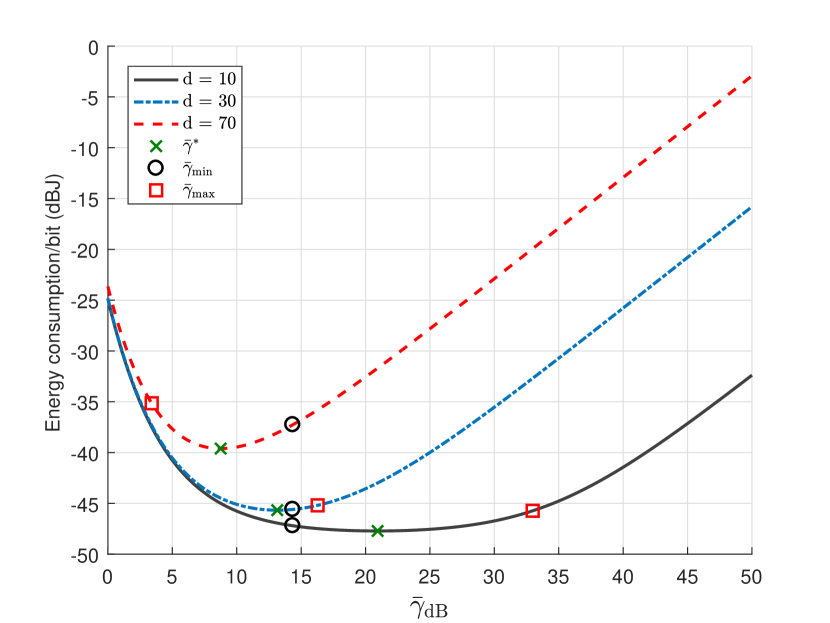
Figure 2: Optimal SNR vs required SNR for 4-QAM under reliability constraints of $\varepsilon=0.001$, $\tau_{r}^{\max}=3$ and maximum transmit power of $P_{0}=10$mW.

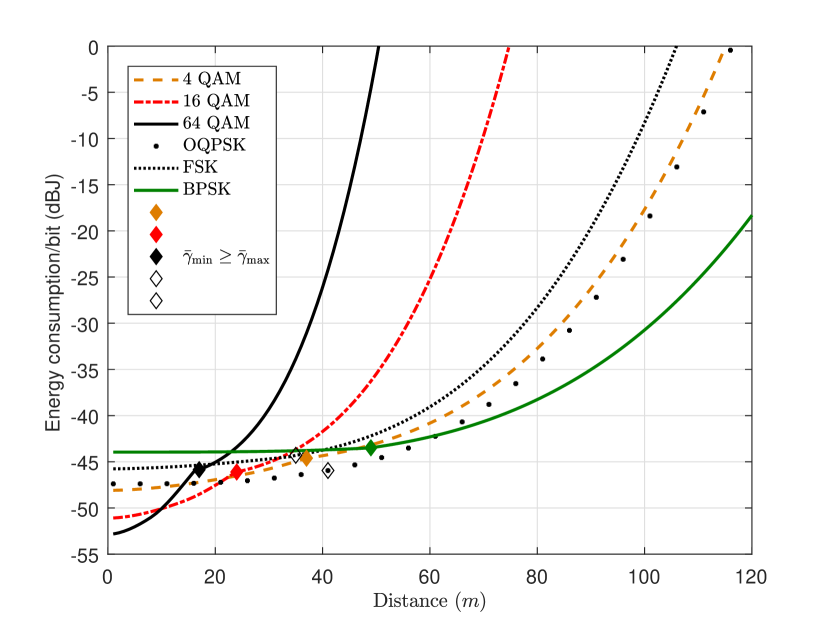
Figure 3: Energy consumption of the modulation schemes with optimal required SNR at each distance. The marked condition $\bar{\gamma}_{\min}\geq\bar{\gamma}_{\max}$ shows the distance beyond which the reliability constraints are not satisfied. Simulation parameters: $P_{0}=10$mW, $\varepsilon=0.001$, $\tau_{r}^{\max}=3$, $n_{p}=984$, $n_{h}=40$.

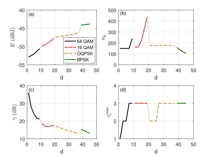
Figure 4: Optimal parameters at the output of the joint optimization algorithm: (a) energy consumption, (b) payload size (bits), (c) SNR, (d) number of retransmissions. The simulation parameters are the same as in Fig. 3.

IV Conclusions

In this paper, we studied the cross-layer link optimization while ensuring energy efficiency and reliability constraints. For cross-layer analysis, we first presented a simple approximation to average PER in block fading channels. The proposed PER approximation is in the form elementary functions, and maintains an explicit connection between the physical/link layer parameters and the packet error rate. The numerical analysis confirms the tightness of the approximation as compared to earlier studies. Later, we exploited the proposed PER approximation in the energy consumption model to find energy optimal yet reliability and hardware compliant conditions for unconstrained optimal SNR and payload size. These conditions are shown to be useful to: i) find optimal SNR for a system with fixed modulation scheme and payload size, ii) develop an holistic algorithm to jointly optimize the physical and link layer parameters.

References

- [1] G. Durisi, T. Koch, and P. Popovski, “Toward massive, ultrareliable, and low-latency wireless communication with short packets,” Proc. of IEEE, vol. 104, no. 9, pp. 1711–1726, Sept 2016.
- [2] C. E. Shannon, “A mathematical theory of communication,” Bell Syst. Tech. J., vol. 27, no. 3, pp. 379–423, 1948.
- [3] Q. Liu, S. Zhou, and G. B. Giannakis, “Cross-layer combining of adaptive modulation and coding with truncated ARQ over wireless links,” IEEE Trans. W. Commun., vol. 3, no. 5, pp. 1746–1755, 2004.
- [4] F. Rosas and C. Oberli, “Modulation and SNR optimization for achieving energy-efficient communications over short-range fading channels,” IEEE Trans. W. Commun., vol. 11, no. 12, pp. 4286–4295, 2012.
- [5] Y. Xi, A. Burr, J. Wei, and D. Grace, “A general upper bound to evaluate packet error rate over quasi-static fading channels,” IEEE Trans. W. Commun., vol. 10, no. 5, pp. 1373–1377, 2011.
- [6] S. Liu, X. Wu, Y. Xi, and J. Wei, “On the throughput and optimal packet length of an uncoded ARQ system over slow Rayleigh fading channels,” IEEE Commun. Lett., vol. 16, no. 8, pp. 1173–1175, 2012.
- [7] J. Wu, G. Wang, and Y. R. Zheng, “Energy efficiency and spectral efficiency tradeoff in type-I ARQ systems,” IEEE J. Sel. A. in Commun., vol. 32, no. 2, pp. 356–366, 2014.
- [8] A. Mahmood and R. Jäntti, “Packet error rate analysis of uncoded schemes in block-fading channels using extreme value theory,” IEEE Commun. Lett., vol. 21, no. 1, pp. 208–211, Jan 2017.
- [9] S. Cui, A. J. Goldsmith, and A. Bahai, “Energy-constrained modulation optimization,” IEEE Trans. W. Commun., vol. 4, no. 5, pp. 2349–2360, 2005.
- [10] T. Wang, W. Heinzelman, and A. Seyedi, “Minimization of transceiver energy consumption in wireless sensor networks with AWGN channels,” in 46th Conf. on Commun., Control, and Computing, 2008, pp. 62–66.
- [11] Y. Hou, M. Hamamura, and S. Zhang, “Performance tradeoff with adaptive frame length and modulation in wireless network,” in 5th Intl. Conf. on Computer and Inf. Tech. IEEE, 2005, pp. 490–494.
- [12] M. Wu et al., “New exponential lower bounds on the Gaussian Q-function via Jensen’s inequality,” in IEEE Veh. Tech. Conf., 2011.