Localized dark solitons and vortices in defocusing media with spatially inhomogeneous nonlinearity
Abstract
Recent studies have demonstrated that defocusing cubic nonlinearity with local strength growing from the center to the periphery faster than , in space of dimension with radial coordinate , supports a vast variety of robust bright solitons. In the framework of the same model, but with a weaker spatial-growth rate, with , we here test the possibility to create stable localized continuous waves (LCWs) in one- and two-dimensional (1D and 2D) geometries, localized dark solitons (LDSs) in 1D, and localized dark vortices (LDVs) in 2D, which are all realized as loosely confined states with a divergent norm. Asymptotic tails of the solutions, which determine the divergence of the norm, are constructed in a universal analytical form by means of the Thomas-Fermi approximation (TFA). Global approximations for the LCWs, LDSs, and LDVs are constructed on the basis of interpolations between analytical approximations available far from (TFA) and close to the center. In particular, the interpolations for the 1D LDS, as well as for the 2D LDVs, are based on a “deformed-tanh” expression, which is suggested by the usual 1D dark-soliton solution. The analytical interpolations produce very accurate results, in comparison with numerical findings, for the 1D and 2D LCWs, 1D LDSs, and 2D LDVs with vorticity . In addition to the 1D fundamental LDSs with the single notch, and 2D vortices with , higher-order LDSs with multiple notches are found too, as well as double LDVs, with . Stability regions for the modes under the consideration are identified by means of systematic simulations, the LCWs being completely stable in 1D and 2D, as they are ground states in the corresponding settings. Basic evolution scenarios are identified for those vortices which are unstable. The settings considered in this work may be implemented in nonlinear optics and in Bose-Einstein condensates.
pacs:
05.45.Yv, 42.65.Tg, 42.65.Jx, 03.75.LmI Introduction
It is commonly believed that the formation of localized waves (alias solitons) in uniform media is a result of the balance between diffraction and self-focusing or defocusing nonlinearity FPC . Following this concept, it has been established that defocusing nonlinearity creates dark solitons, while the self-focusing nonlinearity is necessary for the existence of bright solitons in homogeneous media.
The situation may be different in inhomogeneous media. First, inhomogeneity can be represented by spatially periodic linear potentials, induced by photonic crystals in optics PC , by gratings built into plasmonic waveguides for surface plasmon waves plasmon , and by optical lattices in atomic Bose–Einstein condensates (BECs) BEC ; BEC-Rev1 ; BEC-Rev2 or Fermi gases Fermi . Owing to the straightforward realization in a vast variety of physical systems, periodic potentials play an increasingly important role in manipulations of different kinds of waves and solitons G-Assanto ; Peli . It has been demonstrated that the periodic potentials, in a combination with the self-focusing or defocusing material nonlinearity, give rise to various species of bright solitons BEC-Rev1 ; BEC-Rev2 ; soliton-Rev1 ; soliton-Rev2 ; soliton1 ; soliton2 , including ordinary ones, residing in the semi-infinite gap of the system’s linear spectrum, and gap solitons in finite bandgaps. In particular, the formation of bright gap solitons in the system with the defocusing sign of the nonlinearity may be interpreted as a result of the reversal of the sign of the effective dispersion under the action of the periodic potential uniform-GS -Salerno .
Another possibility for the creation of bright solitons is offered by nonlinear lattices (see a review NL and references therein). These are nonlinear counterparts of linear periodic potentials, which are induced by spatially periodic modulations of the local strength and, possibly, sign of the nonlinearity. In optics, nonlinear lattices may be engineered by means of properly designed photonic-crystal structures (e.g., filling voids in photonic crystals by solid Russell or liquid phot-cryst materials with different values of the Kerr coefficient, or the coefficient accounting for the quadratic nonlinearity chi^2 ). Another possibility is to use inhomogeneous distributions of nonlinearity-enhancing dopants dopant (note, in particular, that appropriate dopants may induced defocusing on top of a self-focusing background Gaetano ). In BEC, similar nonlinearity landscapes can be induced by the Feshbach resonance in spatially nonuniform optical nonuniform-Feshbach or magnetic Feshbach-magnetic fields. In the framework of one-dimensional (1D) settings, nonlinear lattices support bright solitons under various conditions soliton-NL .
On the contrary to the commonly adopted principle that pure defocusing nonlinearities, without the help of linear potentials, cannot produce bright solitons, it was demonstrated that media with a pure self-repulsive (defocusing) spatially inhomogeneous nonlinearity, whose local strength grows from the center to the periphery at any rate faster than ( is the radial coordinate), can support a great variety of robust self-trapped modes in the space of dimension , including 1D fundamental and higher-order (dipole and multipole) solitons, 2D solitary vortices with arbitrarily high topological charges soliton-Defo1 , as well as sophisticated 3D modes, such as soliton gyroscopes Defo9 and skyrmions, i.e., vortex rings with intrinsic twist Defo8 . Such modes exist due to the balance between the spatially inhomogeneous repulsive nonlinearity and linear dispersion/diffraction. A characteristic feature of these self-trapped modes is nonlinearizability of the underlying equations for their decaying tails, in contrast to the usual bright solitons in media with uniform or periodically modulated nonlinearities, where solitons are restricted to the semi-infinite or finite bandgaps of the corresponding linear spectrum BEC-Rev1 ; BEC-Rev2 ; soliton-Rev1 ; soliton-Rev2 ; soliton1 ; soliton2 . In fact, the nonlinearizability of the tails makes the concept of the linear spectrum irrelevant for the solitons supported by repulsive nonlinearities with the spatially growing local strength.
The exploration of bright solitons and solitary vortices supported by such a scheme has been extended to a variety of physical settings, see Refs. soliton-Defo1 -Defo13 and references therein. However, all the studies in this field were, thus far, restricted to the above-mentioned condition of the steep spatial modulation of the self-defocusing, whose local strength must grow with faster than . Actually, this condition secures the convergence of the soliton’s total norm for bright solitons. Weakly localized states, possible in the presence of a more gentle modulation, with , have not been studied yet. Because their total norm diverges (they are localized too loosely for the convergence of the norm), like in the usual continuous-wave states and dark solitons dark , such spatially even (symmetric) and odd (antisymmetric) modes may be considered, respectively, as localized continuous-wave (LCW) states, and as localized dark solitons (LDSs). In particular, the LCW configurations represent the ground state in the present settings. The consideration of this system is relevant, as it may be easier to implement a gentle modulation profile in the experiment than its above-mentioned steep counterpart, and the LDS offers an essential extension of the well-elaborated concept of dark solitons in the uniform 1D space dark . This is the subject of the present work. We here focus on 1D and 2D media with the defocusing cubic nonlinearity subject to the moderate spatial modulation. In these settings, 1D LDS solutions and 2D vortex modes (localized dark vortices, LDVs) with vorticity can be obtained in an approximate analytical form, which is validated by comparison with numerical results. More complex states, such as higher-order1D solitons and vortices with , are constructed numerically.
The paper is organized as follows. In Sec. II, we introduce the model and report approximate analytical solutions. Tails of the weakly localized states are produced in a universal form, which does not depend on the spatial dimension, nor on the parity (spatial symmetry or antisymmetry) of the underlying solution, by the Thomas-Fermi approximation (TFA). For the global structure of the LCWs, LDSs, and LDVs we develop approximations based on interpolations between asymptotic forms available close to the center and far from it. In particular, a “deformed-tanh” interpolation produces quite accurate results for 1D LDS and 2D LDV with . In Sec. III, numerical results are reported for the shape and stability of 1D fundamental and higher-order LCWs and LDSs. Numerical findings for 2D states are presented in Sec. IV. The paper is concluded by Sec. V.
II The model and analytical approximations
II.1 The underlying equations
The model is based on the generalized nonlinear Schrödinger (NLS) or Gross-Pitaevskii equation for the mean-field wave function , written in the scaled form:
| (1) |
The mode is cast in the optics notation, with the evolution variable, , realized as the propagation distance (for matter waves, is replaced by time, ), being the local strength of the defocusing cubic term, which is specified below, and Laplacian acts on transverse coordinates in the bulk medium, with . Stationary solutions to Eq. (1) with real propagation constant are sought for as , where the stationary wave function (generally speaking, it may be complex) obeys its own equation:
| (2) |
Equation (2) can be derived from the respective Lagrangian,
| (3) |
The 1D model corresponds to an obvious one-dimensional reduction of Eqs. (1)-(3)
To illustrate the concept of the loosely localized solitons, we note that the 2D version of Eq. (2) with
| (4) |
which corresponds to the critical case of , gives rise to a family of weakly singular exact LDV solutions with vorticity :
| (5) |
where is the angular coordinate, and wavenumber may take any negative value.
II.2 The Thomas-Fermi approximation
In the framework of the TFA, which neglects derivatives in stationary equation (2), it gives rise to real self-trapped solutions in the form of
| (6) |
which is relevant at large , where it is asymptotically exact, i.e.,
| (7) |
soliton-Defo1 . Because the defocusing nonlinearity implies , Eq. (6) holds for , cf. exact vortex solution (5). The TFA produces universal results for the tails, which, as mentioned above, do not depend on the spatial dimension, nor on the global structure of the underlying solution [e.g., whether it is an LCW, or a fundamental LDS, or its higher-order counterpart (see below), or an LDV].
For modulation profiles which have a power-law asymptotic form at ,
| (8) |
with ( is realized as for ), Eq. (6) gives rise to slowly decaying tails in the form of
| (9) |
where the second term in the parentheses represents the first post-TFA correction, that corroborates relation (7). It follows from Eq. (9) that the critical point, , which separates states with convergent and divergent values of the norm (or integral power, in terms of optics), , is an exact one (the correction to the TFA does not affect this point).
The divergence of for can be estimated by introducing an overall size, , of a truncated version of the system, with (obviously, any physical system has a finite size). Then, Eq. (6) yields
| (10) |
for or ( is written here, as is negative), which explicitly displays the divergence at . In the limit case of , Eq. (10) is replaced by
| (11) |
where is an internal size of the mode; for instance, it is for vortex (14), see below. We note that, while the truncation, of course, determines the dependence in the case of , it does not strongly affect the shape of the modes under the consideration, if is large enough, as the shapes of the modes decays at large anyway, even if relatively slowly. This conclusion is corroborated, in particular, by the shapes displayed below in Figs. 1, 3, 6 and 8.
It is worthy to note that expressions (10) and (11) satisfy the anti-Vakhitov-Kolokolov (anti-VK) condition, , which is a necessary stability condition for localized modes supported by defocusing nonlinearities antiVK . In fact, the anti-VK condition is sufficient for the stability of ground states, but it may not be sufficient for excited states, see below.
In the 2D version of the model, LDVs states with integer vorticity are looked for as
| (12) |
with real amplitude obeying the following equation:
| (13) |
For taken as per Eq. (4), and , an exact solution of Eq. (13) is given by Eq. (5). In the general case, a solution to Eq. (13) can again be looked for by means of the TFA, neglecting the radial derivatives:
| (14) |
cf. the application of the TFA to vortex solutions in Refs. TFA ; Defo9 .
II.3 Global interpolations
The TFA is relevant for the outer zone, where the derivatives (diffraction, in the optics model, or kinetic energy, in the BEC system) may be neglected. As an attempt to construct a global approximation, we will try an interpolation which goes over into the TFA at large , and matches a correct analytical form of the solution in its inner zone. The interpolation for the LCW (the ground state), corresponding to the modulation profile (8), is based on the following simplest expression, which is compatible with the TFA asymptotic form (6) and the fact that the LCW state must be free of singularities and feature a maximum at :
| (15) |
This expression does feature spatial dimension (recall that is replaced by in 1D). However, the value of constant , which is determined by the substitution of this expression in Eq. (2) at (or , in the 1D case), depends on the :
| (16) |
In fact, interpolation (15) may be used for the bright solitons at too, although in that case it turns out to be less accurate, see below.
It is relevant to calculate the total norm of the truncated version () of expression (15) with for (for the analytical result is too cumbersome):
| (17) | |||
| (18) |
Obviously, in the limit of , expressions (17) and (18) carry over into Eqs. (10) and (11), respectively, produced by the TFA.
For the 2D LDV with vorticity , as well as for the 1D LDS, a natural form of the interpolation, that we call “deformed tanh”, is suggested by the hyperbolic-tangent solution for the usual dark soliton in the 1D uniform space:
| (19) |
where determines the radius of the LDS core, which is used below as a fitting parameter, while comparing Eq. (19) to numerical results. In the 1D geometry, in Eq. (19) is replaced by
| (20) |
while is replaced by as the argument of and .
Below, results produced by numerical computations are displayed and compared to these analytical approximations. We stress that the validity of the numerical schemes needs to be carefully checked in the present setting, as properly handling boundary conditions (b.c.) for weakly localized modes with slowly decaying tails is a known challenging problem in simulations of nonlinear partial differential equations, such as the NLS equation (1). In particular, we have inferred that the usual split-step fast Fourier transform method with periodic b.c. does not apply to the present model, and the finite-difference method with Neumann or Dirichlet b.c. is not an appropriate one either. To resolve the issue, we have developed a finite-difference method with dynamical b.c. for robust simulations of Eq. (1). These b.c. are defined as , where subscripts and pertain to the boundary point and the inner one adjacent to it (more technical details will be presented elsewhere). It is relevant to mention that our numerical codes correctly reproduce 1D and 2D bright solitons (with finite norms) for , which were found in earlier works soliton-Defo1 , Defo5 -Defo10 .
III Numerical results for one-dimensional localized modes
In this section we report numerical results for the 1D model with modulation profile (8), in which is fixed by means of rescaling. The LCW and LDS states (both fundamental and higher-order ones, in the latter case) were produced as numerical solutions of stationary equation (2). The same stationary solutions can also be found by means of integrating NLS equation (1) in imaginary time, fixing propagation constant , which is another well-known numerical method for producing stationary solutions IT . The stability of the so found solutions was then checked by means of systematic simulations of Eq. (1) for the evolution of perturbed solutions in real time, using the above-mentioned finite-difference numerical scheme with the dynamical b.c. The spatial and time steps were taken as and , using different sizes of the integration domain, which are appropriate in different cases, as specified below.
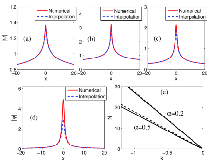
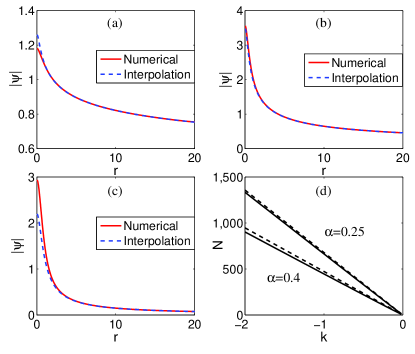
Numerical simulations reveal that the shape of 1D LCW states conspicuously change with the increase of the nonlinearity-modulation power, , featuring growth of the amplitude and decrease of the width. Naturally, the LCW states carries over into a fundamental bright soliton, with the convergent norm, at . These features are clearly seen in Figs. 1(a-d). Comparison between the numerical solutions for the 1D LCW states and the analytical approximation based on Eqs. (15) and (16) is shown in Figs. 1 too. It is seen that the LCW profiles predicted by the analytical interpolation provide a good fit to their numerical counterparts for all , and the corresponding expression (10) for the norm, calculated in the truncated domain, also well matches the numerically computed dependences, in spite of the absence of any fitting parameter in the underlying interpolation [on the contrary to the presence of parameter in Eqs. (19) and (20), which is used below in Fig. 3]. A discrepancy in the analytical and numerical shapes of the localized mode occurs at for bright solitons, although the wings are still well approximated by the analytical ansatz in Fig. 1(d), which is explained by its compliance with the asymptotically exact expression (6). In the latter case, the discrepancy is naturally explained by the fact that the smooth interpolation formula cannot accurately follow effects of the steep modulation.
Direct simulations demonstrate that all the 1D LCW states found at , as well as their bright-soliton continuation at , are completely stable, in accordance with the fact that they represent the system’s ground state. In addition, as seen in Fig. 1(e), relations at different values of obey the above-mentioned anti-VK criterion, , which provides the necessary stability condition for the localized modes in the defocusing medium; it is actually a sufficient one for ground states antiVK .
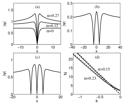
Examples of 1D fundamental (single-notch) LDSs, with different values of the modulation power , are displayed in Fig. 2(a). It is seen that the solitons’ amplitude increases, the waist shrinks, and the decaying tails sharpen with the increase of . The curves for the families of 1D fundamental LDSs, shown in Fig. 2(d), along with their TFA-predicted counterparts, given by Eq. (10), are obtained for the truncated 1D system with , covered by a grid of points, cf. Eq. (10). A (relatively small) mismatch between the numerical and TFA curves is explained by the fact that the TFA ignores the norm defect induced by the notch.
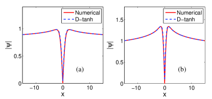
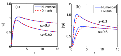
The comparison of typical numerically found profiles of the 1D fundamental LDSs with their counterparts provided by the deformed-tanh interpolation (19) is presented in Fig. 3. It shows that the approximation is very accurate, provided that the value of in ansatz (19) is selected as one which yields the best fit of the analytically predicted LDS profile to the numerical one.
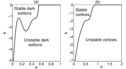
Results for the stability analysis of the fundamental LDSs, collected in Fig. 4(a), demonstrate that they are stable at
| (21) |
for values of which are not too large. Typical examples of the evolution of stable and unstable 1D fundamental LDSs are displayed in Figs. 5(a) and 5(b), respectively. As can be seen in the latter figure, the unstable fundamental LDS spontaneously loses its spatial antisymmetry (i.e., the notch, at which was originally vanishing, gets filled), and quickly evolves into an excited (oscillating) version of the LCW, i.e., a disturbed ground state, with a maximum, rather than minimum, of , at .
It is relevant to stress that the conclusions concerning the stability of the 1D LDSs, produced by the simulations performed in the domain of size , as shown in Fig. 5, are virtually the same as obtained using a smaller domain (not shown here in detail), , (which is still essentially larger than the size of the corresponding LDSs), the shape of the respective stability area remaining the same in Fig. 4(a). It is also relevant to stress that in those cases when the LDSs are unstable [Fig. 5(c,d)], the instability is clearly seen to set in the central segment of the integration domain, rather than arriving from the periphery. These findings confirm that conclusions about the stability of the LDSs in the infinite system may be based on the simulations performed in finite domains, in spite of the divergence of the total norm in the infinite system. The same conclusions are valid for the 2D setting. In particular, conclusions concerning the instability boundary and development of 2D vortices (see Fig. 9 below) are virtually the same for the domain with size and for a smaller one (not shown in detail here) of size . In the latter case, the instability remains confined too to the central core of the integration domain.
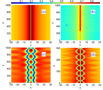
A noteworthy property of the 1D model is the existence of excited states in the form of higher-order LDSs which are defined by the number of the profile’s zero-crossings (notches), starting from the single one for the fundamental LDS. As is well known, the integrable NLS equation, corresponding to , does not give rise to higher-order dark solitons. Typical examples of the second- and third-order LDSs are displayed in Figs. 2(b) and 2(c), respectively.
All the higher-order LDSs are unstable, but the instability may be weak. As shown in Fig. 5(c) and 5(d), weakly unstable higher-order dark solitons develop regular spatially symmetric oscillations, keeping the initial number of notches. These plots clearly demonstrate that the instability of the higher-order LDSs is explained by the interaction between individual notches.
IV Numerical results for two-dimensional localized continuous-wave and dark-vortex modes
In this section we focus on 2D LCW states and 2D LDVs, the latter representing the most interesting modes in the 2D geometry. Noteworthy results are obtained for the modes of both types.
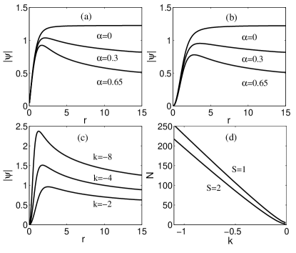
The comparison of the analytical interpolation for the LCW, based on Eqs. (15) and (16), with the numerically found solutions is shown in Fig. 6(a,b,c). Outer segments of the analytical shapes completely overlap with their numerical counterparts, while the inner ones show minor discrepancies at smaller and larger values of . Note that, similar to the 1D LCWs [see Fig. 1(a-c)], good accuracy is provided by the analytical interpolation without the use of any fitting parameter. At , the 2D LCW state carries over into the fundamental bright soliton, which was found in Ref. soliton-Defo1 . Similar to those 1D counterparts, the 2D LCW states are found to be completely stable in their entire existence region, , which is easily explained by the fact that they are ground states of the 2D setting.
Examples of LDVs with vorticities and are plotted, respectively, in Figs. 7(a) and (b). Both subplots include the standard dark vortex in the uniform space, with vortex ; TFA , for the sake of comparison. It is seen that, with the increase of , the shape of the weakly localized vortex sharpens, for both and , similar to the trend featured by the 1D LDS in Fig. 2(a). On the other hand, the amplitude of the vortex decreases, while in Fig. 2(a) it was increasing with the growth of . The deformed-tanh interpolation (19) may be accurately fitted to the numerically found shape of the LDVs with as shown in Fig. 8(a).
Results of the stability tests for perturbed LDVs with are collected in Fig. 4(b). The vortices are stable at [cf. Eq. (21)], for values of which are not too large. A stability area was also found for the LDVs with (in particular, it is bounded by ), but its exact delineation requires excessively heavy simulations.
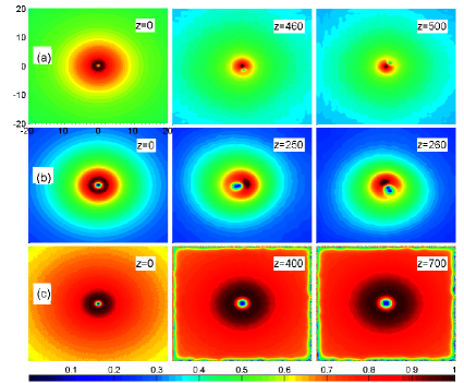
Different unstable vortices feature different scenarios of the instability development. In Fig. 9(a), an unstable LDV with transforms into an eccentric vortex, with the pivot moving along a circular trajectory. Furthermore, in Fig. 9(b) an unstable double vortex () splits into a rotating pair of unitary ones, which is typical for multiple vortices in self-defocusing media vortex . Lastly, in Fig. 9(c), the perturbed double vortex (again, the one with ) spontaneously broadens and turns into a different, apparently stable, double LDV. The latter scenario was found to be typical for the evolution of the LDVs which are unstable because their is too large.
V Conclusion
It has recently been demonstrated that, opposite to the common belief, the pure defocusing nonlinearity can support various robust bright solitons in the space of dimension , provided that the local strength of the nonlinearity increases from the center to the periphery faster than . In previous works, only bright-soliton modes were theoretically investigated in settings of this type. In this work, we have addressed loosely localized modes, with the divergent norm, hence they may be categorized as LCWs, LDSs, and LDVs (localized continuous waves, localized dark solitons, and localized dark vortices, respectively). Such modes are supported by the local nonlinearity strength growing slower than, or exactly as, . The corresponding nonlinearity landscapes may be realized for light waves in nonlinear photonic crystals or in inhomogeneously doped optical media, and for matter waves in BEC, controlled by means of the spatially inhomogeneous Feshbach resonance. The LCWs, which represent the ground state in the 1D and 2D geometries, LDSs (both fundamental and higher-order ones, characterized by multiple notches in the 1D case), and LDVs, with vorticities and , have been constructed by means of analytical approximations and numerical methods. The relevant analytical methods are the TFA (Thomas-Fermi approximation) for universal tails of all modes, and the interpolation between analytical approximations available far from and close to the center, for the LCW states in 1D and 2D, as well as for 1D LDS and 2D LDV. In particular, the interpolation based on the deformed-tanh expression provides for a very accurate fit to numerically found 1D LDS and 2D LDV profiles (the latter one fits well for ). Stability areas for these modes, and instability development scenarios for unstable ones, have been identified by means of systematic simulations of the perturbed evolution. In particular, the LCWs are completely stable in 1D and 2D alike, which is readily explained by the fact that they serve as ground states in the respective settings.
In terms of BEC, the present analysis may be extended for the 3D setting, with in Eq. (8). On the other hand, it may be interesting to extend the analysis to loosely localized states in 1D and 2D models with spatially modulated nonlocal nonlinearity, where, in particular, the stabilization of vortex solitons is also a relevant problem nonlocal .
VI Acknowledgment
We appreciate valuable discussions with G. Assanto. The work of J. Z. is supported by NSFC, China (project Nos. 61690222,61690224,11204151), by the Initiative Scientific Research Program of the State Key Laboratory of Transient Optics and Photonics, and partially by the Youth Innovation Promotion Association of the Chinese Academy of Sciences (project No. 2016357) and the CAS/SAFEA International Partnership Program for Creative Research Teams. The work of B. A. M. is supported, in part, by grant No. 2015616 from the joint program in physics between the National Science Foundation (US) and Binational (US-Israel) Science Foundation.
References
- (1) Y. S. Kivshar and G. P. Agrawal, Optical Solitons: From Fibers to Photonic Crystals (Academic, San Diego, CA, 2003).
- (2) J. D. Joannopoulos, S. G. Johnson, J. N. Winn, and R. D. Meade, Photonic Crystals: Molding the Flow of Light (Princeton University Press: Princeton, 2008).
- (3) L. Dal Negro and S. V. Boriskina, Laser Phot. Rev. 6, 178 (2012).
- (4) C. J. Pethick and H. Smith, Bose-Einstein condensate in dilute gas (Cambridge University Press: Cambridge, 2008).
- (5) V. A. Brazhnyi and V. V. Konotop, Mod. Phys. Lett. B 18, 627 (2004).
- (6) O. Morsch and M. Oberthaler, Rev. Mod. Phys. 78, 179 (2006).
- (7) H. T. C. Stoof, K. B. Gubbels, and D. B. M. Dickerscheid, Ultracold Quantum Fields (Springer: Dordrecht, 2009).
- (8) G. Assanto, A. Fratalocchi and M. Peccianti, Opt. Exp. 15, 5248 (2007); F. Lederer, G. I. Stegeman, D. N. Christodoulides, G. Assanto, M. Segev, and Y. Silberberg, Phys. Rep. 463, 126 (2008).
- (9) J. Yang, Nonlinear Waves in Integrable and Nonintegrable Systems (SIAM: Philadelphia, 2010); D. E. Pelinovsky, Localization in Periodic Potential: From Schrödinger Operators to the Gross-Pitaevskii Equation (Cambridge University Press: Cambridge, 2011).
- (10) B. A. Malomed, D. Mihalache, F. Wise, and L. Torner, J. Optics B 7, R53 (2005).
- (11) Y. V. Kartashov, V. A. Vysloukh, and L. Torner, Progress in Optics 52, 63 (ed. by E. Wolf: North Holland,Amsterdam, 2009).
- (12) B. B. Baizakov, B. A. Malomed, and M. Salerno, Europhys. Lett. 63, 642 (2003).
- (13) J. Yang and Z. H. Musslimani, Opt. Lett. 28, 2094 (2003).
- (14) D. E. Pelinovsky, A. A. Sukhorukov, and Y. S. Kivshar, Phys. Rev. E 70, 036618 (2004).
- (15) Y. V. Kartashov, B. A. Malomed, and L. Torner, Rev. Mod. Phys. 83, 247 (2011).
- (16) B. B. Baizakov, V. V. Konotop, and M. Salerno, J. Phys. B 35, 5105 (2002); E. A. Ostrovskaya and Yu. S. Kivshar, Phys. Rev. Lett. 90, 160407 (2003).
- (17) F. Luan, A. K. George, T. D. Hedley, G. J. Pearce, D. M. Bird, J. C. Knight, and P. S. J. Russell, Opt. Lett. 29, 2369 (2004).
- (18) A. Ferrando, M. Zacarés, P. Fernandez de Cordoba, D. Binosi, and J. A. Monsoriu, Opt. Express 11, 452 (2003); T. I. Larsen, A. Bjarklev, D. S. Hermann, and J. Broeng, ibid. 11, 2589 (2003); A. Fuerbach, P. Steinvurzel, J. A. Bolger, A. Nulsen, and B. J. Eggleton, Opt. Lett. 30, 830 (2005); C. R. Rosberg, F. H. Bennet, D. N. Neshev, P. D. Rasmussen, O. Bang, W. Krolikowski, A. Bjarklev, and Y. S. Kivshar, Opt. Express 15, 12145 (2007); P. Dalgaard Rasmussen, F. H. Bennet, D. N. Neshev, A. A. Sukhorukov, C. R. Rosberg, W. Krolikowski, O. Bang, and Y. S. Kivshar, Opt. Lett. 34, 295 (2009).
- (19) K. Gallo and G. Assanto, Opt. Lett. 32, 3149 (2007); K. Gallo, A. Pasquazi, S. Stivala and G. Assanto, Phys. Rev. Lett. 100, 053901 (2008).
- (20) J. Hukriede, D. Runde, and D. Kip, J. Phys. D 36, R1 (2003).
- (21) A. Piccardi, A. Alberucci, N. Tabiryan and G. Assanto, Opt. Lett. 36, 1456 (2011).
- (22) R. Yamazaki, S. Taie, S. Sugawa, and Y. Takahashi, Phys. Rev. Lett. 105, 050405 (2010); M. Yan, B. J. DeSalvo, B. Ramachandhran, H. Pu, and T. C. Killian, ibid. 110, 123201 (2013); L. W. Clark, L.-C. Ha, C.-Y. Xu, and C. Chin, ibid. 115, 155301 (2015).
- (23) S. Ghanbari, T. D. Kieu, A. Sidorov, and P. Hannaford, J. Phys. B: At. Mol. Opt. Phys. 39, 847 (2006); O. Romero-Isart, C. Navau, A. Sanchez, P. Zoller, and J. I. Cirac, Phys. Rev. Lett. 111, 145304 (2013).
- (24) Y. Sivan, G. Fibich, B. Ilan, and M. I. Weinstein, Phys. Rev. E 78, 046602 (2008); N. V. Hung, P. Ziń, M. Trippenbach, and B. A. Malomed, ibid. 82, 046602 (2010); J. Zeng and B. A. Malomed, Phys. Rev. A 85, 023824 (2012).
- (25) O. V. Borovkova, Y. V. Kartashov, L. Torner, and B. A. Malomed, Phys. Rev. E 84, 035602(R) (2011).
- (26) R. Driben, Y. V. Kartashov, B. A. Malomed, T. Meier, and L. Torner, Phys. Rev. Lett. 112, 020404 (2014).
- (27) Y. V. Kartashov, B. A. Malomed, Y. Shnir, and L. Torner, Phys. Rev. Lett. 113, 264101 (2014).
- (28) Q. Tian, L. Wu, Y. Zhang, and J.-F. Zhang, Phys. Rev. E 85, 056603 (2012).
- (29) J. Zeng and B. A. Malomed, Phys. Rev. E 86, 036607 (2012).
- (30) Y. Wu, Q. Xie, H. Zhong, L. Wen, and W. Hai, Phys. Rev. A 87, 055801 (2013).
- (31) R. Driben, Y. V. Kartashov, B. A. Malomed, T. Meier, and L. Torner, New J. Phys. 16, 063035 (2014).
- (32) D. Guo, J. Xiao, L. Gu, H. Ji, and L. Dong, Physica D 343, 1 (2017).
- (33) Y. S. Kivshar and B. Luther-Davies, Phys. Rep. 298, 81 (1998); D. J. Frantzeskakis, J. Phys. A: Math. Theor. 43, 213001 (2010).
- (34) H. Sakaguchi and B. A. Malomed, Phys. Rev. A 81, 013624 (2010).
- (35) M. L. Chiofalo, S. Succi, and M. P. Tosi, Phys. Rev. E 62, 7438 (2000); X. Antoine, W. Baoc, and C. Besse, Comp. Phys. Commun. 184, 2621 (2013).
- (36) A. L. Fetter, Rev. Mod. Phys. 81, 647 (2009); Phys. Rev. A 89, 023629 (2014).
- (37) J. C. Neu, Physica D 43, 385 (1990); G. A. Swartzlander, Jr., and C. T. Law, Phys. Rev. Lett. 69, 2503 (1992).
- (38) A. I. Yakimenko, Y. A. Zaliznyak, and Y. S. Kivshar, Phys. Rev. E 71, 065603(R) (2005); G. Assanto, A. A. Minzoni and N. F. Smyth, Opt. Lett. 39, 509 (2014); Y. V. Izdebskaya, G. Assanto and W. Królikowski, ibid. 40, 4182 (2015); Y. V. Izdebskaya, W. Królikowski, N. F. Smyth, and G. Assanto, J. Optics 18, 054006 (2016).