Thermalization of Isolated Bose-Einstein Condensates by Dynamical Heat Bath Generation

Abstract

If and how an isolated quantum system thermalizes despite its unitary time evolution is a long-standing, open problem of many-body physics. The eigenstate thermalization hypothesis (ETH) postulates that thermalization happens at the level of individual eigenstates of a system’s Hamiltonian. However, the ETH requires stringent conditions to be validated, and it does not address how the thermal state is reached dynamically from an initial non-equilibrium state. We consider a Bose-Einstein condensate (BEC) trapped in a double-well potential with an initial population imbalance. We find that the system thermalizes although the initial conditions violate the ETH requirements. We identify three dynamical regimes. After an initial regime of undamped Josephson oscillations, the subsystem of incoherent excitations or quasiparticles (QP) becomes strongly coupled to the BEC subsystem by means of a dynamically generated, parametric resonance. When the energy stored in the QP system reaches its maximum, the number of QPs becomes effectively constant, and the system enters a quasi-hydrodynamic regime where the two subsystems are weakly coupled. In this final regime the BEC acts as a grand-canonical heat reservoir for the QP system (and vice versa), resulting in thermalization. We term this mechanism dynamical bath generation (DBG).

I Introduction

Isolated quantum systems pose a challenging problem of quantum physics due to the unclear mechanism of how these systems reach thermal behavior, as was experimentally observed Trotzky2012 ; Gring2012 ; Polkovnikov2011 ; Yukalov2011 . The experimental results contradict the common knowledge that unitary time evolution of an initial pure state, $|\Psi(t)\rangle=e^{-iHt}|\Psi(0)\rangle$, prohibits entropy maximization, and as a consequence thermalizaiton should not take place. A number of quantum thermalization scenarios have been put forward.

One of the most prominent conjectures is the eigenstate thermalization hypothesis (ETH) which suggests that thermalization happens at the level of individual eigenstates Deutsch1991 ; Srednicki1994 . The ETH became very popular after its numerical verification for hard-core bosons in two-dimensional lattices Rigol2008 ; ETH_review , albeit some systems where it fails have been identified Pozsgay2014 . The ETH is typically restricted to the observation of local quantities.

The ETH has been found to be valid even in some integrable systems Alba2015 , although thermalization is known in general not to occur in such cases. The concept of thermalization was adapted to systems with non-ergodic dynamics (e.g. integrable systems), by generalized Gibbs ensembles imposing multiple conservation laws on average ETH_review . A separate branch of research has evolved around prethermalization dynamics Kollath2007 ; Kehrein2008 ; Kollar2011 ; Joerg_review which occur in nearly integrable systems with small, integrability-breaking perturbations.

We pursue a different, more generally applicable route to thermalization. If an isolated quantum system is sufficiently complex, more precisely, if the many-body Hilbert space dimension is sufficiently high, then it is not possible by any experiment to determine all quantum numbers of a state. The set of measured quantum numbers defines a subspace of the total many-body Hilbert space. This subspace will be called subsystem, while the remaining subspace of undetermined quantum numbers will serve as a thermal bath or reservoir. The subsystem is then described by a reduced density matrix with the reservoir (undetermined) quantum numbers traced out. This reduced density matrix will correspond to a statistically mixed state, since the system Hilbert space and the reservoir Hilbert space are in general entangled. This situation is identical to the canonical or grand canonical ensemble of an open subsystem coupled to the reservoir. In fact, it was shown that any such subsystem of the total system is described by the canonical thermal ensemble for the overwhelming majority of pure states of the total system Goldstein2006 ; Reimann2015 . Thus, according to the second law of thermodynamics and in spite of the unitary time evolution of the total system, the subsystem will evolve for long times to the density matrix of a (grand) canonical ensemble in thermodynamic equilibrium.

In the present article we not only study a thermalized state of a subsystem in the long-time limit, but we review how such a thermal state is reached dynamically. We show that the thermalization dynamics mentioned above is quite general, if only the Hilbert space dimension, i.e., the particle number, is large enough. The coupling between bath and subsystem need not be weak, and it is not necessary to define separate energy eigenstates of the subsystem and of the bath Goldstein2006 . No restrictions on the initial state (like narrow energy distribution) apply. Most importantly, it is even valid in cases where either the bath or the subsystem Hilbert space is initially not populated, i.e., the bath is dynamically generated by the total system’s time evolution, possibly involving multiple time scales Mauro2009 ; Mauro2015 ; Anna2016 . We thus term this thermalization dynamics “dynamical bath generation” (DBG). The DBG mechanism can be understood also as a setup where the subsystem-bath coupling evolves in time. Initially the coupling constant is zero (the "bath" is absent), whereas during the bath-generation process the coupling constant reaches its maximum and subsequently decays to small, constant values. It is in this final regime when one can refer to the total system as being separated into two subsystems, each serving as a heat reservoir for the other.

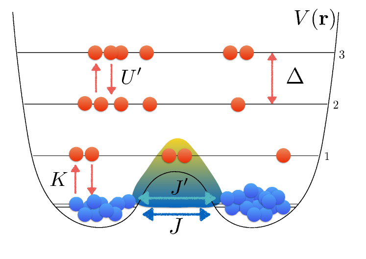
Figure 1: Schematic view of a condensate in a double well potential $V(\mathbf{r})$. The blue dots represent atoms in the condensate, while the red dots depict incoherent excitations (quasiparticles) out of the condensate. The figure visualizes the energy spacing of trap levels $\Delta$, the bare Josephson coupling $J$ as well as the quasiparticle-assisted Josephson tunnelling $J^{\prime}$ and the interaction $U$ between particles in different levels (see text for more details). Note that the single-particle levels shown are, in general, strongly renormalized by the interactions.

Cold atomic systems are favorable candidates for studying the problem of closed system thermalization as they can be sufficiently isolated from the environment and possess an unprecedented degree of tunability. They offer the possibility to realize abrupt changes of almost any of the system parameters (parameter "quenches") thus driving the system out of equilibrium in a controlled way. As a generic system we consider a Bose-Einstein condensate (BEC) of cold atoms trapped in a double-well potential (Bose Josephson junction, see Fig. 1), with initially all atoms in the two single-particle ground states of the two wells with a population imbalance $z$. We quench the Josephson coupling from $0$ to a finite value $J$ and study the resulting dynamics by non-equilibrium quantum field theory methods. Interestingly, we identify several time scales which govern the non-equilibrium physics, see Fig. 2. First, Josephson oscillations without damping can occur up to a time $t=\tau_{c}$ after the quench Mauro2009 ; Mauro2015 . During a time interval $\tau_{c}<t<\tau_{f}$ the condensate (BEC) and the quasiparticle (QP) subsystems are strongly coupled via a dynamically generated, parametric resonance, indicated by the BEC and the QP spectra being strongly correlated with each other Anna2016 . In this regime incoherent excitations are thus created out of the condensate in an avalanche-like manner. However, at a freeze-out time $\tau_{f}$ the BEC dynamics effectively decouple from the QP subsystem by virtue of total energy conservation, and the BEC and the QP spectra become uncorrelated. For $t>\tau_{f}$ slow, exponential relaxation to thermal equilibrium with a relaxation time $\tau_{th}$ occurs due to weak coupling of the QP subsystem to the BEC as a grand canonical reservoir, and vice-versa Anna2016 .

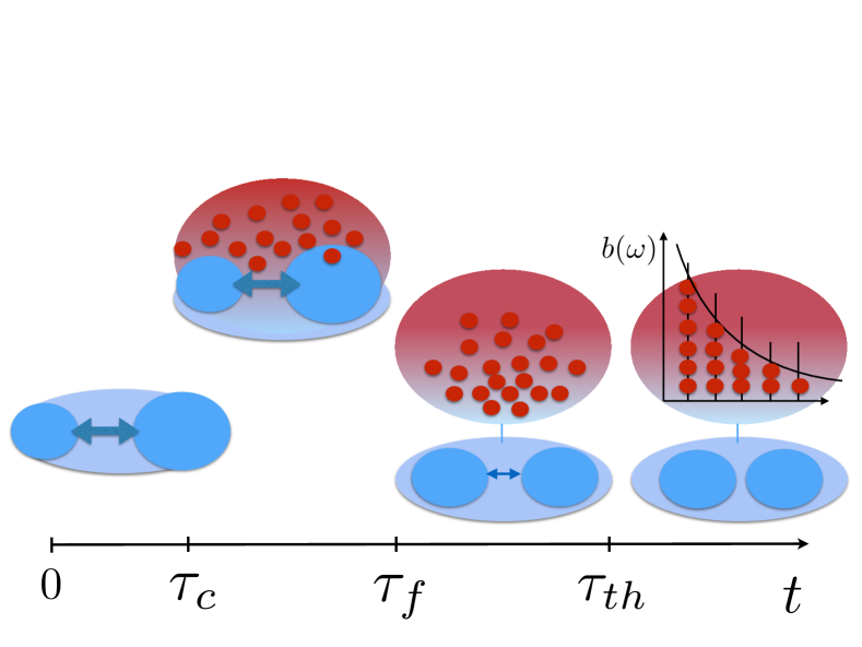
Figure 2: Different time-scales involved in the thermalization of an oscillating Bose gas trapped in a double-well potential. $\tau_{c}$ is the characteristic time scale associated with the creation of incoherent excitations which drastically influence the non-equilibrium BEC dynamics. For $\tau_{c}<t<\tau_{f}$ the BEC and QP subsystems are strongly coupled, while for $t>\tau_{f}$ an effective decoupling takes place imposed by energy conservation. Thermalization occurs with a slow relaxation rate for $t>t_{f}$ where the QP subsystem serves as an external bath for the BEC and visa versa. The oscillating BECs are depicted in blue, incoherent excitations as red dots.

The article is structured as follows. In section II we review in some detail the ETH and discuss its restrictive assumptions and resulting limitations. Section III contains the representation of the many-body model Hamiltonian of the Bose gas in the basis of trap eigenstates as well as the detailed description of the time-dependent Keldysh-Bogoliubov method used to compute the dynamics of the coupled system of BEC and incoherent excitations. The results are discussed in section IV, describing in detail the three different time regimes that are involved in the thermalization process of this system. Concluding remarks are given in section V.

II Ergodicity and the Eigenstate Thermalization Hypothesis

The ETH provides, within its realm of validity, an explanation why isolated quantum systems can behave thermally. It also constitutes an attempt at a microscopic, first-principles derivation of the ergodic theorem, the basis of equilibrium statistical mechanics. Therefore, in this section we briefly recall the ergodic theorem and then describe the line of arguments constituting the ETH. We also inspect critically the conditions that are necessary for this line of arguments to be valid.

As is well known from statistical mechanics (see e.g. Landau ), thermalization of a closed system, isolated from the environment, is rooted in the assumption of ergodicity. The ergodic theorem of classical statistical mechanics states that the statistical or ensemble average $\langle A\rangle$ of a physical observable $A$ is equivalent to its long time average $\overline{A(p,q)}$,

$$\langle A\rangle = \frac{1}{N!(2\pi\hbar)^{3N}}\int dpdq\rho(p,q)A(p,q)$$ (1)

$$= \lim_{t\rightarrow\infty}\frac{1}{t}\int_{0}^{t}dt^{\prime}A(p(t^{\prime}),q(t^{\prime}))=\overline{A}\ .$$

Here, $N$ is the number of particles in the system, $p$ and $q$ are phase space coordinates (collectively denoting the coordinates for all $N$ particles), and $\rho(p,q)$ is the distribution of the microcanonical ensemble. For the purpose of proper normalization, the quasiclassical assumption has been employed that the particles are indistinguishable and that the phase space volume per particle is equal to $(2\pi\hbar)^{3}$. A rigorous derivation of the ergodic assumption Eq. (1) has been achieved only in special cases, but a general derivation is still lacking Khinchin ; Sinai . In statistical physics the following heuristic argument is often used Landau : Consider a small but still macroscopic subsystem $S_{1}$ of a given closed system. Let $\Delta p\Delta q$ be a small volume in phase space. Then during a sufficiently long time interval $t$ the subsystem $S_{1}$ will "visit" $\Delta p\Delta q$ and will spend there some finite time $\Delta t$, so that we can always define a finite probability density

$$\Delta W=\lim_{t\rightarrow\infty}\frac{\Delta t}{t},$$ (2)

for $S_{1}$ to be found in the volume $\Delta p\Delta q$. In this case, it is plausible that Eq. (1) will be satisfied with a corresponding probability distribution of $\Delta W$, see also Birkhoff ; Neumann ; Singh .

To extend these ideas and concepts to the quantum case, consider now a quantum system described by the Hamiltonian $H$ prepared in an initial state $|\Psi(0)\rangle$. The initial state can be expanded in a complete orthonormal basis $\{|\psi_{n}\rangle\}$ of eigenstates of the Hamiltonian,

$$H|\psi_{n}\rangle = E_{n}|\psi_{n}\rangle,\$$

$$|\Psi(0)\rangle = \sum_{n}c_{n}|\psi_{n}\rangle,$$ (3)

with the normalization $\sum_{n}|c_{n}|^{2}=1$. The ETH states that for a physical observable $\hat{A}$, under certain conditions to be discussed below, the long-time avarage of the expectation value $\langle\Psi(t)|\hat{A}|\Psi(t)\rangle$ in a many-body state $|\Psi(t)\rangle$ is indistinguishable from the thermal average $\langle A\rangle_{mc}(E)$ in the microcanonical ensemble with a fixed energy $E$,

$$\overline{A}:=\lim_{t\rightarrow\infty}\frac{1}{t}\int_{0}^{t}dt^{\prime}\langle\Psi(t^{\prime})|\hat{A}|\Psi(t^{\prime})\rangle\stackrel{{\scriptstyle!}}{{=}}\langle A\rangle_{mc}(E)\ .$$ (4)

The ETH scenario proceeds as follows. For a closed system, the unitary time evolution of $|\Psi(t)\rangle$ can be expanded in the basis of energy eigenstates,

$$|\Psi(t)\rangle=\sum_{n}c_{n}e^{-\frac{i}{\hbar}E_{n}t}|\psi_{n}\rangle,$$ (5)

and the expectation value of $A$ at time $t$ reads,

$$\langle\Psi(t)|\hat{A}|\Psi(t)\rangle=\sum_{nm}c_{n}^{*}c_{m}e^{-\frac{i}{\hbar}(E_{m}-E_{n})t}A_{nm},$$ (6)

with the matrix elements $A_{nm}=\langle\psi_{n}|\hat{A}|\psi_{m}\rangle$. Assuming that (i) the vast majority of the energy eigenvalues are non-degenerate, the off-diagonal terms in Eq. (6) are oscillatory and will vanish in the long-time average. One obtains

$$\overline{A}=\lim_{t\rightarrow\infty}\frac{1}{t}\int_{0}^{t}dt^{\prime}A(t^{\prime})=\sum_{n}|c_{n}|^{2}A_{nn}.$$ (7)

In order to define a microcanonical ensemble with energy $E$ it is now necessary to assume that (ii) the distribution of the energy eigenvalues in the expansion Eq. (5) around the average $E$ is sufficiently narrow, where the width

$$\Delta E=\frac{1}{{\cal N}}\sqrt{\sum_{n}^{\cal N}(E_{n}-E)^{2}}$$ (8)

is small on a macroscopic scale, i.e., $\Delta E\ll E$, but large enough so that there is a large number of energy eigenstates $|\psi_{n}\rangle$ within $\Delta E$. As two crucial conditions, one furthermore assumes that (iii) the matrix elements $A_{nn}$ of the observable $\hat{A}$ depend continuously on the energy eigenvalues $E_{n}$ and (iv) they do essentially not depend on any other quantum numbers describing the state, see Fig. 3. If the conditions (ii), (iii) and (iv) are satisfied, then not only the energy eigenvalues $E_{n}$, but also the $A_{nn}$ have a small variation, i.e., they can be assumed constant within the set of $|\psi_{n}\rangle$ contributing to the system’s state vector $|\Psi(t)\rangle$,

$$A_{nn}\approx A_{E}+\frac{dA_{nn}}{dn}dn=A_{E}+\frac{dA_{nn}}{dn}\frac{(E_{n}-E)}{dE_{n}/dn}\approx A_{E}$$ (9)

Here, $A_{E}=\langle\psi_{E}|\hat{A}|\psi_{E}\rangle$ is the matrix element for an energy eigenstate with the energy $E$ and $|E_{n}-E|\leq\Delta E\ll E$. Thus, the time average from Eq. (7) can be written approximately as

$$\overline{A}\approx\sum_{n}|c_{n}|^{2}A_{E}=A_{E}\ .$$ (10)

Note that the right-hand side of Eq. (10) does not depend on details of the initial conditions, but only on the typical energy $E$ of the eigenstates composing $|\Psi(t)\rangle$. On the other hand, the microcanonical average of $A$ is

$$\langle A\rangle_{mc}(E)=\frac{1}{\Omega}\sum_{n:E_{n}\in[E-\Delta E/2,E+\Delta E/2]}A_{nn}$$ (11)

where $\Omega$ is the number of eigenstates in the narrow energy interval $[E,E+\Delta E]$ in the limit $\Delta E\to 0$. Combining Eqs. (9), (10) and (11) it follows that the long-time average $\overline{A}$ is equal to the quantum mechanical expectation value $A_{E}$ of one representative energy eigenstate and, hence, to the microcanonical average,

$$\overline{A}\approx A_{E}\approx\langle A\rangle_{mc}(E).$$ (12)

This is the statement of the ETH. It means that the equilibrium thermodynamics of an observable $\hat{A}$ is described by its expectation value $A_{E}$ with respect to a typical energy eigenstate or by its long-time average. If Eq. (12) holds, the system is called quantum ergodic Deutsch1991 ; Rigol2012 .

Figure 3: Visualization of the conditions necessary for the ETH to be valid. In addition to being (essentially) non-degenerate (i), the energy eigenvalues $E_{n}$ must have a narrow spread $\Delta E$ around their mean value (ii). Furthermore, within the interval $\Delta E$ the $A_{nn}$ must not vary strongly (iii), i.e., they should depend continuously on $E_{n}$, and they must be independent of other quantum numbers (iv), see text. This defines a hypersurface (blue) in the space spanned by all quantum numbers and the expectation values $A_{nn}$. It is narrow along the $E_{n}$ axis and flat along all other directions. The ETH scenario applies if the vast majority of all $A_{nn}$ lie on this hypersurface.

However, severe conditions have to be imposed in order to reach this conclusion, as seen above:

• Non-degeneracy of the vast majority of many-body eigenenergies $E_{n}$.
  

• Narrow distribution of the eigenenergies $E_{n}$ around a mean value $E$ on a macroscopic scale:
  $|E_{n}-E|\lesssim\Delta E<<E$.
  

• Within the width $\Delta E$ all diagonal matrix elements of the observable $\hat{A}$ are approximately equal: $A_{nn}\approx A_{E}$.
  

• These diagonal elements $A_{nn}$ do not depend independently on quantum numbers other than the energy eigenvalues $E_{n}$.
  

We now discuss the impact of these assumptions on the applicability of the ETH to physical systems. Conditions (i) and (ii) tend to mutually exclude each other at first sight. A narrow distribution of the $E_{n}$ is needed in order to define the microcanonical ensemble, but the eigenenergies $E_{n}$, $E_{m}$ of different states ($n\neq m$) must differ sufficiently in order for the offdiagonal terms in Eq. (6) to average out in the long-time average. One expects a relaxation time of the order of $1/\Delta E$ which can be macroscopically large. This is in contrast to the fast thermalization rates that are usually observed, unless conservation laws inhibit thermalization, and that are not controlled by $\Delta E$ but by the coupling energies of the Hamiltonian (see, e.g., Fig. 16 and Ref. Anna2016 ). Condition (ii) also restricts the type of initial states to which ETH thermalization can apply to those with a narrow energy spectrum $\Delta E$. By contrast, many types of initial states, for instance single-level occupation number eigenstates that appear naturally as the initial conditions of Josephson trap systems (see below), have a broad energy spectrum. While condition (iii) is plausible for a system without a phase transition, condition (iv) clearly imposes a serious restriction on the observables that may obey the ETH. It is difficult to specify general types of such observables.

Because of these difficulties in finding general criteria for the applicability of the ETH, it has been tested for specific systems using numerical methods, such as exact diagonalization Rigol2008 ; Roux2009 , time-dependent dynamical mean-field theory (tDMFT) Werner2014 ; Werner2015 , density matrix and renormalization group (DMRG) Schollwoeck2005 ; Kollath2007 . In addition, alternative scenarios of thermalization have been put forward, see, e.g., Yukalov2011 ; Rigol2012 or Polkovnikov2011 for a review.

III Formalism

III.1 Hamiltonian

Our goal is to describe Josephson oscillations between weakly-coupled bosonic condensates including effects of quasiparticles. The Josephson effect was originally predicted in superconductors Josephson1962 , and by now is well studied theoretically Javanainen1986 ; Smerzi1997 as well as experimentally Albiez2005 ; Levy2007 . Despite a lot of progress there still exist unresolved issues with the experimental results. For example, although in Ref. Albiez2005 several undamped Josephson oscillations were clearly observed, in other experiments Thywissen2011 the Josephson particle current was rapidly suppressed. We suggest the quasiparticle damping mechanism to play a crucial role in such a behaviour. Below we present a formalism Mauro2009 ; Mauro2015 ; Anna2016 which, when applied to specific systems, will shed light on this issue and other problems related to thermalization of isolated closed systems.

In order to describe a bosonic Josephson junction we start from a weakly interacting Bose gas in a double well potential described by the well-known Hamiltonian

$$H=\int d{\bf r}\hat{\Psi}^{\dagger}({\bf r},t)\left(-\frac{\nabla^{2}}{2m}+V_{ext}({\bf r},t)\right)\hat{\Psi}({\bf r},t)$$ (13)

$$+\frac{g}{2}\int d{\bf r}\hat{\Psi}^{\dagger}({\bf r},t)\hat{\Psi}^{\dagger}({\bf r},t)\hat{\Psi}({\bf r},t)\hat{\Psi}({\bf r},t),$$

where $\hat{\Psi}({\bf r},t)$ is a bosonic field operator, and a contact repulsive interaction is implied with the coupling constant $g=4\pi a_{s}/m$ with $a_{s}$ being the s-wave scattering length. $V_{ext}({\bf r},t)$ is the external double-well trap potential, which in our case is time dependent. We assume that the barrier between the wells is initially infinitely high, so that the Josephson tunneling between the wells is negligible. At $t=0$ the barrier is abruptly lowered down and a sizeable Josephson current will be induced as a result. Such a time dependence of the external potential corresponds to the quenching of the Josephson coupling between the wells, which we can express as

$$J(t)=J\Theta(t),$$ (14)

where $\Theta(t)$ is the Heaviside step function. The quenching of $J$ results in lowering of the ground state energy of the system by the $\Delta E=J\sqrt{N_{1}(0)N_{2}(0)}$, where $N_{1}(0)$ and $N_{2}(0)$ are initial occupation numbers of the two wells, which can be quite large. Hence, after the quench two initially separated condensates will be found in an excited state $\Delta E$ above the coupled ground state. We will show that, depending on the system parameters, this energy can suffice to excite quasiparticles out of the BECs with time-dependent BEC amplitude playing the role of a perturbation on the QP system. The QPs will be excited to higher lying discrete energy levels of the double-well potential, while the two lowest states of the potential are occupied by the BECs.

Before deriving the equations of motion for the field operators $\hat{\Psi}({\bf r},t)$ and $\hat{\Psi}({\bf r},t)^{\dagger}$, we expand the operators in terms of a complete basis $\mathds{B}=\{\varphi_{-},\varphi_{+},\varphi_{1},\varphi_{2},\dots\varphi_{M}\}$ of the exact single-particle eigenstates of the double well potential $V_{ext}({\bf r},t>0)$, i.e. just after the coupling between the wells is turned on. Note that the ground state wavefunction has a zero in the barrier between the wells, thus minimizing its energy, i.e., for a symmetric double-well, it is parity antisymmetric, while the first excited state is symmetric. Hence, we denote the ground state wavefunction of the double well by $\varphi_{-}$, the first excited state wavefunction by $\varphi_{+}$, the second excited state by $\varphi_{1}$ and so on. The field operator in the eigenbasis of the double-well potential is then

$$\hat{\Psi}({\bf r},t)=\phi_{1}({\bf r})\hat{b}_{01}(t)+\phi_{2}({\bf r})\hat{b}_{02}(t)+\sum_{n=1}^{M}\varphi_{n}({\bf r})\hat{b}_{n}(t)\ ,$$ (15)

where we have applied the transformation, $\hat{b}_{01}(t)=(\hat{b}_{-}+\hat{b}_{+})/\sqrt{2}$, $\hat{b}_{02}(t)=(\hat{b}_{-}-\hat{b}_{+})/\sqrt{2}$ on the operators $\hat{b}_{\pm}(t)$ for particles in the $\varphi_{\pm}$ subspace, with the wavefunctions $\phi_{1}({\bf r})=(\varphi_{-}({\bf r})+\varphi_{+}({\bf r}))/\sqrt{2}$ and $\phi_{2}({\bf r})=(\varphi_{-}({\bf r})-\varphi_{+}({\bf r}))/\sqrt{2}$. Since the $\varphi_{+}({\bf r})$ ($\varphi_{-}({\bf r})$) have the same (the opposite) sign in the two wells, the $\phi_{1,2}({\bf r})$ are localized in the left or right well, respectively, i.e., they approximately constitute the ground state wavefunctions of the left and right well. We now assume the Bogoliubov prescription for the operators describing condensates in each well

$$\hat{b}_{0\alpha}(t)\to a_{\alpha}(t)=\sqrt{N_{\alpha}(t)}e^{i\theta_{\alpha}(t)},$$ (16)

$\alpha=1,2$, where $N_{\alpha}$ and $\theta_{\alpha}$ are the number of particles and the phase of the condensate in the left (right) well of the potential. The field operator finally reads,

$$\hat{\Psi}({\bf r},t)=\phi_{1}({\bf r})a_{1}(t)+\phi_{2}({\bf r})a_{2}(t)+\sum_{n=1}^{M}\varphi_{n}({\bf r})\hat{b}_{n}(t).$$ (17)

The Bogoliubov substitution neglects phase fluctuations in the ground states of each of the potential wells, while the full quantum dynamics is taken into account for the excited states, $\varphi_{n}$, $n=1,\ 2,\dots,\ M$ (in the numerical evaluations we will limit the number of levels which can be occupied by the QPs to $M=5$.). This is justified when the BEC particle numbers are sufficiently large, $N_{\alpha}\gg 1$, e.g., for the experiments Albiez2005 . When the quantum dynamics due to excitations to upper levels is neglected, only the first two terms from Eq. (17) contribute, which is equivalent to a semiclassical two-mode approximation for a condensate in a double well Milburn1997 ; Smerzi1997 ; Gati2007 . The applicability of the semiclassical approximation has been discussed in detail in Refs. Zapata03 ; Zapata98 ; Pitaevskii01 and has been tested experimentally in Ref. Esteve08 .

We also note that the definition of excited single-particle states is not obvious in the case of a condensate trapped in a double-well Smerzi2003 ; Gati_diss with the width of the wave-function being in general a function of the number of particles in the well, or total number of particles. Various solutions to this problem and applicability of the approximations are discussed in detail in Ref. Ananikian2006 . This issue, however, does not play an important role for the physics we discuss in this work, and we therefore proceed with the expansion (17).

We can now derive the Hamiltonian of our setup in terms of two condensate amplitudes and quasiparticle operators $\hat{b},\hat{b}^{\dagger}$. For $t>0$ the Hamiltonian consists of three contributions

$$H=H_{coh}+H_{J}+H_{coll}.$$ (18)

$H_{coh}$ includes all local contributions, i.e. all terms which are bi-linear in the $\hat{b}_{n}$-operators and local in the well index $\alpha=1,\ 2$,

$$H_{coh}=\varepsilon_{0}\sum_{\alpha=1}^{2}a_{\alpha}^{*}a_{\alpha}+\frac{U}{2}\sum_{\alpha=1}^{2}a_{\alpha}^{*}a_{\alpha}^{*}a_{\alpha}a_{\alpha}+\sum_{n=1}^{M}\varepsilon_{n}\hat{b}_{n}^{\dagger}\hat{b}_{n}$$

$$+K\sum_{\alpha=1}^{2}\sum_{n,m=1}^{M}\left[a_{\alpha}^{*}a_{\alpha}\hat{b}_{n}^{\dagger}\hat{b}_{m}+\frac{1}{4}(a_{\alpha}^{*}a_{\alpha}^{*}\hat{b}_{n}\hat{b}_{m}+h.c.)\right],$$ (19)

where $U$ and $K$ are positive interaction constants, and $\varepsilon_{n}$ are the energies of the $M$ equidistant levels of the double well, separated by the trap frequency, $\varepsilon_{n}=n\Delta$. For simplicity we neglect hereafter a possible level-dependence of the coupling constants. We coin the part of the Hamiltonian $H_{coh}$ "coherent" since it describes only the single-particle dynamics of QPs and therefore cannot lead to a decoherence of QPs.

$H_{J}$ includes all Josephson-like terms, which are still coherent but are non-local in the well index,

$$H_{J} = -J(a_{1}^{*}a_{2}+a_{2}^{*}a_{1})+J^{\prime}\sum_{n,m=1}^{M}\left[(a_{1}^{*}a_{2}+a_{2}^{*}a_{1})\hat{b}_{n}^{\dagger}\hat{b}_{m}\right.$$ (20)

$$+ \left.\frac{1}{2}(a_{1}^{*}a_{2}^{*}\hat{b}_{n}\hat{b}_{m}+h.c.)\right]\ .$$

The terms proportional to $J$ are standard Josephson terms also known from the semiclassical approximation Gati2007 , while terms proportional to $J^{\prime}$ describe novel QP-assisted Josephson tunneling events between the wells (see Fig. 1).

The non-linear collisional terms $H_{coll}$ account for full many-body interactions,

$$H_{coll}=\frac{U^{\prime}}{2}\sum_{n,m=1}^{M}\sum_{l,s=1}^{M}\hat{b}_{m}^{\dagger}\hat{b}_{n}^{\dagger}\hat{b}_{l}\hat{b}_{s}\hskip 93.89418pt$$ (21)

$$+R\left[\sum_{\alpha=1}^{2}\sum_{n,m,s=1}^{M}a_{\alpha}^{*}\hat{b}_{n}^{\dagger}\hat{b}_{m}\hat{b}_{s}+\sum_{\alpha,\beta,\gamma=1}^{2}\sum_{n=1}^{M}a^{*}_{\alpha}a^{*}_{\beta}a_{\gamma}\hat{b}_{n}+h.c.\right]$$

We have introduced the set of parameters in the Hamiltonian (18):

$$\varepsilon_{0} = \int d{\bf r}\left[\frac{\hbar^{2}}{2m}|\nabla\phi_{1,2}({\bf r})|^{2}+\phi_{1,2}^{2}V_{ext}({\bf r})\right],$$

$$U = g\int d{\bf r}\,|\phi_{1,2}({\bf r})|^{4},$$

$$\varepsilon_{n} = \int d{\bf r}\,\varphi_{n}({\bf r})\left(-\frac{\nabla^{2}}{2m}+V_{ext}({\bf r})\right)\varphi_{n}({\bf r}),$$

$$U^{\prime} = g\int d{\bf r}\,\varphi_{n}({\bf r})\varphi_{m}({\bf r})\varphi_{l}({\bf r})\varphi_{s}({\bf r}),$$

$$J = -2\int d{\bf r}\left[\frac{\hbar^{2}}{2m}(\nabla\phi_{1}\nabla\phi_{2})+\phi_{1}\phi_{2}V_{ext}({\bf r})\right],$$

$$K = 2K_{11nm}=2K_{22nm},$$

$$J^{\prime} = 2K_{12nm}=2K_{21nm},$$

$$R = g\int d{\bf r}\phi_{\alpha}({\bf r})\varphi_{n}({\bf r})\varphi_{m}({\bf r})\varphi_{s}({\bf r}),$$ (22)

with $K_{\alpha\beta nm}=g\int d{\bf r}\,\phi_{\alpha}({\bf r})\phi_{\beta}({\bf r})\varphi_{n}({\bf r})\varphi_{m}({\bf r})$.

We will now use the standard non-equilibrium field-theoretical techniques Rammerbook ; Kadanoffbook ; Griffinbook to calculate time-dependence of the following observables: condensate population imbalance

$$z(t)=\frac{N_{1}(t)-N_{2}(t)}{N_{1}(t)+N_{2}(t)},$$ (23)

the phase difference between the BECs, $\theta(t)=\theta_{2}(t)-\theta_{1}(t)$ and the QP occupation numbers $n_{1}(t),\ n_{2}(t),\ \dots,n_{M}(t)$.

III.2 General Quantum Kinetic Equations

The time-dependence of the observables can be calculated from the kinetic equations for the Green’s functions of the interacting Bose gas within the Kadanoff-Baym framework Rammerbook ; Kadanoffbook ; Griffinbook . As usual, it is convenient to separate the non-equilibrium Green function into its classical and quantum counterparts and then derive the equations of motion (Dyson equations) for them in the standard way. The classical part ${\bf C}_{\alpha\beta}(t,t^{\prime})$ is expressed in terms of classical condensate amplitudes $a_{1}(t)$ and $a_{2}(t)$

$${\bf C}_{\alpha\beta}(t,t^{\prime})=-i\left(\begin{matrix}a_{\alpha}(t)a_{\beta}^{*}(t^{\prime})&a_{\alpha}(t)a_{\beta}(t^{\prime})\\ a_{\alpha}^{*}(t)a_{\beta}^{*}(t^{\prime})&a_{\alpha}^{*}(t)a_{\beta}(t^{\prime})\end{matrix}\right),$$ (24)

while the quantum part is written in terms of quasiparticle operators $\hat{b}_{n},\hat{b}_{n}^{\dagger}$

$${\bf G}_{nm}(t,t^{\prime}) = -i\left(\begin{matrix}\langle T_{C}\hat{b}_{n}(t)\hat{b}_{m}^{\dagger}(t^{\prime})\rangle&\langle T_{C}\hat{b}_{n}(t)\hat{b}_{m}(t^{\prime})\rangle\\ \langle T_{C}\hat{b}_{n}^{\dagger}(t)\hat{b}_{m}^{\dagger}(t^{\prime})\rangle&\langle T_{C}\hat{b}_{n}^{\dagger}(t)\hat{b}_{m}(t^{\prime})\rangle\end{matrix}\right)$$ (25)

$$= \left(\begin{matrix}G_{nm}(t,t^{\prime})&F_{nm}(t,t^{\prime})\\ \overline{F}_{nm}(t,t^{\prime})&\overline{G}_{nm}(t,t^{\prime})\end{matrix}\right).$$

Here $\hat{T}_{C}$ is time-ordering along the Keldysh contour. Note that at this stage we have already assumed that the position dependence of the Green functions is absorbed in the parameters (22) (for details see Mauro2015 ).

The general structure of the Dyson equations for these Green’s functions is the following

$$\int_{C}d\overline{t}\left[{\bf G}_{0}^{-1}(t,\overline{t})-{\bf S}^{HF}(t,\overline{t})\right]{\bf C}(\overline{t},t^{\prime})$$

$$=\int_{C}d\overline{t}\,{\bf S}(t,\overline{t}){\bf C}(\overline{t},t^{\prime}),$$ (26)

$$\int_{C}d\overline{t}\left[{\bf G}_{0}^{-1}(t,\overline{t})-{\bf\Sigma}^{HF}(t,\overline{t})\right]{\bf G}(\overline{t},t^{\prime})=\mathds{1}\delta(t-t^{\prime})$$

$$+\int_{C}d\overline{t}\,{\bf\Sigma}(t,\overline{t}){\bf G}(\overline{t},t^{\prime}).$$ (27)

The term proportional to $\delta(t-t^{\prime})$ is absent in Eq. (26) because of the classical nature of the condensate amplitudes. In the Eqs. (26) and (27) we separated the first order in interaction Hartree-Fock self-energies ${\bf S}^{HF},{\bf\Sigma}^{HF}$ from their second order collisional counterparts ${\bf S},{\bf\Sigma}$. The operator ${\bf G}_{0}^{-1}$ is defined as

$${\bf G}_{0}^{-1}(t,\overline{t})=\delta(t-\overline{t})\left[i\tau_{3}\frac{\partial}{\partial t}-\left(-\frac{1}{2m}\Delta_{1}+V_{ext}(t)\right)\mathds{1}\right],$$ (28)

where

$$\tau_{3}=\begin{pmatrix}1&0\\ 0&-1\end{pmatrix}.$$ (29)

All self-energies, including the later appearing ${\bm{\gamma}},{\bm{\Gamma}}$ and ${\bm{\Pi}}$ have the same $2\times 2$ structure in the Bogoliubov space

$${\bf S}(t,t^{\prime})=\left(\begin{matrix}S^{G}(t,t^{\prime})&S^{F}(t,t^{\prime})\\ S^{\overline{F}}(t,t^{\prime})&S^{\overline{G}}(t,t^{\prime})\end{matrix}\right),$$ (30)

where superscripts $G,F,...$ are references to the corresponding normal and anomalous Green functions in Eq. (25).

We rewrite the contour integrals in Eqs. (26) and (27) as integrals over the real time axis and get the Dyson equation for the condensate Green’s function in the form

$$\int\limits_{-\infty}^{\infty}d\overline{t}\left[{\bf G}_{0,\alpha\gamma}^{-1}(t,\overline{t})-{\bf S}^{HF}_{\alpha\gamma}(t,\overline{t})\right]{\bf C}_{\gamma\beta}(\overline{t},t^{\prime})=$$

$$-i\int\limits_{-\infty}^{t}d\overline{t}{\bm{\gamma}}_{\alpha\gamma}(t,\overline{t}){\bf C}_{\gamma\beta}(\overline{t},t^{\prime}),$$ (31)

where ${\bm{\gamma}}_{\alpha\beta}={\bm{S}}^{>}_{\alpha\beta}-{\bm{S}}^{<}_{\alpha\beta}$ (the superscripts "<" and ">" refer to the standard non-equilibrium "lesser" and "greater" self-energies Rammerbook ; Griffinbook ), and the bare propagator is given by

$${\bf G}_{0,\alpha\beta}^{-1}(t,t^{\prime})=\left[i\tau_{3}\delta_{\alpha\beta}\frac{\partial}{\partial t}-\mathds{1}E_{\alpha\beta}\right]\delta(t-t^{\prime})\ ,$$ (32)

with $E_{11}=E_{22}=\varepsilon_{0}$ and $E_{12}=E_{21}=-J$. Hereafter Greek indeces, $\alpha,\,\beta=1,\,2$, refer to the condensates in the left and right wells, and latin indices, $n,\,m=1,\,2,\,\dots,\,M$, denote the QP levels, we also imply Einstein summation.

From Eq. (27) we obtain the two equations

$$\int\limits_{-\infty}^{\infty}d\overline{t}\left[{\bf G}_{0,nl}^{-1}(t,\overline{t})-{\bf\Sigma}_{nl}^{HF}(t,\overline{t})\right]{\bf G}_{lm}^{\gtrless}(\overline{t},t^{\prime})=$$

$$-i\left[\int\limits_{-\infty}^{t_{1}}d\overline{t}\,{\bf\Gamma}_{nl}(t,\overline{t}){\bf G}_{lm}^{\gtrless}(\overline{t},t^{\prime})-\int\limits_{-\infty}^{t_{1^{\prime}}}d\overline{t}{\bf\Sigma}_{nl}^{\gtrless}(t,\overline{t}){\bf A}_{lm}(\overline{t},t^{\prime})\right],$$ (33)

with

$${\bf G}_{0,nm}^{-1}(t,t^{\prime})=\left[i\tau_{3}\frac{\partial}{\partial t}-\varepsilon_{n}\mathds{1}\right]\delta_{nm}\delta(t-t^{\prime}),$$ (34)

and

$${\bf G}^{<}(t,t^{\prime})=-i\left(\begin{matrix}\langle\hat{b}^{\dagger}(t^{\prime})\hat{b}(t)\rangle&\langle\hat{b}(t^{\prime})\hat{b}(t)\rangle\\ \langle\hat{b}^{\dagger}(t^{\prime})\hat{b}^{\dagger}(t)\rangle&\langle\hat{b}(t^{\prime})\hat{b}^{\dagger}(t)\rangle\end{matrix}\right)=$$

$$\left(\begin{matrix}G^{<}(t,t^{\prime})&F^{<}(t,t^{\prime})\\ \overline{F}^{<}(t,t^{\prime})&\overline{G}^{<}(t,t^{\prime})\end{matrix}\right),$$ (35)

$${\bf G}^{>}(t,t^{\prime})=-i\left(\begin{matrix}\langle\hat{b}(t)\hat{b}^{\dagger}(t^{\prime})\rangle&\langle\hat{b}(t)\hat{b}(t^{\prime})\rangle\\ \langle\hat{b}^{\dagger}(t)\hat{b}^{\dagger}(t^{\prime})\rangle&\langle\hat{b}^{\dagger}(t)\hat{b}(t^{\prime})\rangle\end{matrix}\right)=$$

$$\left(\begin{matrix}G^{>}(t,t^{\prime})&F^{>}(t,t^{\prime})\\ \overline{F}^{>}(t,t^{\prime})&\overline{G}^{>}(t,t^{\prime})\end{matrix}\right),$$ (36)

For practical reasons it is, however, better to work with equations for the spectral function ${{\bf A}_{nm}}=i({\bf G}_{nm}^{>}-{\bf G}_{nm}^{<})$ and the so-called statistical function (see also Berges_review ; Rey2005 )

$${{\bf F}_{nm}}=\frac{{\bf G}_{nm}^{>}+{\bf G}_{nm}^{<}}{2}=\frac{{\bf G}^{K}_{nm}}{2},$$ (37)

here ${\bf G}^{K}_{nm}$ being the Keldysh component of (25). The introduction of such symmetrized and antisymmetrized two-point correlators is not important if we were to reduce the calculation to the first-order Bogoliubov-Hartree-Fock (BHF) approximation, however, is beneficial for a more general case when second order (in interaction) contributions are taken into account. The derivation then simplifies due to symmetry relations for the propagators and their self-energies, and allows us to rewrite the terms involving higher order processes as "memory integrals".

In the Bogoliubov space these are $2\times 2$ matrices

$${\bf A}_{nm}(t,t^{\prime}) = \left(\begin{array}[]{cc}\text{A}^{G}_{nm}(t,t^{\prime})&\text{A}^{F}_{nm}(t,t^{\prime})\\ \text{A}^{\overline{F}}_{nm}(t,t^{\prime})&\text{A}^{\overline{G}}_{nm}(t,t^{\prime})\end{array}\right),$$ (40)

$${\bf F}_{nm}(t,t^{\prime}) = \left(\begin{array}[]{cc}\text{F}^{G}_{nm}(t,t^{\prime})&\text{F}^{F}_{nm}(t,t^{\prime})\\ \text{F}^{\overline{F}}_{nm}(t,t^{\prime})&\text{F}^{\overline{G}}_{nm}(t,t^{\prime})\end{array}\right).$$ (43)

For further derivations we will extensively use the following symmetry relations for the spectral and statistical functions

$$\text{A}^{\overline{G}}(t,t^{\prime}) = -\text{A}^{G}(t,t^{\prime})^{*}=-\text{A}^{G}(t^{\prime},t),$$

$$\text{A}^{\overline{F}}(t,t^{\prime}) = -\text{A}^{F}(t,t^{\prime})^{*}=\text{A}^{F}(t^{\prime},t)^{*},$$

$$\text{F}^{\overline{G}}(t,t^{\prime}) = -\text{F}^{G}(t,t^{\prime})^{*}=\text{F}^{G}(t^{\prime},t),$$

$$\text{F}^{\overline{F}}(t,t^{\prime}) = -\text{F}^{F}(t,t^{\prime})^{*}=-\text{F}^{F}(t^{\prime},t)^{*}.$$ (44)

The Dyson equations for the spectral and statistical functions are

$$\int\limits_{-\infty}^{\infty}d\overline{t}\left[{\bf G}_{0,n\ell}^{-1}(t,\overline{t})-{\bf\Sigma}_{n\ell}^{HF}(t,\overline{t})\right]{\bf A}_{\ell m}(\overline{t},t^{\prime})=$$

$$-i\int\limits_{t^{\prime}}^{t}d\overline{t}\,{\bf\Gamma}_{n\ell}(t,\overline{t}){\bf A}_{\ell m}(\overline{t},t^{\prime})$$ (45)

$$\int\limits_{-\infty}^{\infty}d\overline{t}\left[{\bf G}_{0,n\ell}^{-1}(t,\overline{t})-{\bf\Sigma}_{n\ell}^{HF}(t,\overline{t})\right]{\bf F}_{\ell m}(\overline{t},t^{\prime})=$$

$$-i\Big{[}\int\limits_{-\infty}^{t}d\overline{t}\,{\bf\Gamma}_{n\ell}(t,\overline{t}){\bf F}_{\ell m}(\overline{t},t^{\prime})$$

$$\quad\quad-\int\limits_{-\infty}^{t^{\prime}}d\overline{t}\,{\bf\Pi}_{n\ell}(t,\overline{t}){\bf A}_{\ell m}(\overline{t},t^{\prime})\Big{]},$$ (46)

where ${\bm{\Pi}}_{nm}=({\bm{\Sigma}}_{nm}^{>}+{\bm{\Sigma}}_{nm}^{<})/2$ and ${\bf\Gamma}_{nm}={\bf\Sigma}_{nm}^{>}-{\bf\Sigma}_{nm}^{<}$. As usual we separated Bogoliubov-Hartree-Fock contributions ${\bf\Sigma}_{nm}^{HF}$ from the second-order contributions describing collisions ${\bf\Sigma}_{nm}$.

Since the BHF contributions are ${\bf S}^{HF}(t,t^{\prime})={\bf S}^{HF}(t)\delta(t-t^{\prime})$, ${\bf\Sigma}^{HF}(t,t^{\prime})={\bf\Sigma}^{HF}(t)\delta(t-t^{\prime})$, we can further simplify the Dyson kinetic equations (31), (45), (46)

$$\left[i\tau_{3}\delta_{\alpha\gamma}\frac{\partial}{\partial t}-\mathds{1}E_{\alpha\gamma}-{\bf S}^{HF}_{\alpha\gamma}(t)\right]{\bf C}_{\gamma\beta}(t,t^{\prime})=$$

$$-i\int\limits_{-\infty}^{t}d\overline{t}{\bm{\gamma}}_{\alpha\gamma}(t,\overline{t}){\bf C}_{\gamma\beta}(\overline{t},t^{\prime}),$$ (47)

$$\left[i\tau_{3}\delta_{n\ell}\frac{\partial}{\partial t}-\varepsilon_{n}\delta_{n\ell}\mathds{1}-{\bf\Sigma}^{HF}_{n\ell}(t)\right]{\bf A}_{\ell m}(t,t^{\prime})=$$

$$-i\int\limits_{t^{\prime}}^{t}d\overline{t}\,{\bf\Gamma}_{n\ell}(t,\overline{t}){\bf A}_{\ell m}(\overline{t},t^{\prime}),$$ (48)

$$\left[i\tau_{3}\delta_{n\ell}\frac{\partial}{\partial t}-\varepsilon_{n}\delta_{n\ell}\mathds{1}-{\bf\Sigma}^{HF}_{n\ell}(t)\right]{\bf F}_{\ell m}(t,t^{\prime})=$$

$$-i\Big{[}\int\limits_{-\infty}^{t}d\overline{t}\,{\bf\Gamma}_{n\ell}(t,\overline{t}){\bf F}_{\ell m}(\overline{t},t^{\prime})$$

$$\quad\quad-\int\limits_{-\infty}^{t^{\prime}}d\overline{t}\,{\bf\Pi}_{n\ell}(t,\overline{t}){\bf A}_{\ell m}(\overline{t},t^{\prime})\Big{]}.$$ (49)

Eqs. (47), (48) and (49) constitute the general equations of motion for the condensate and the non-condensate (spectral and statistical) propagators. They are coupled via the self-energies which are functions of these propagators and must be evaluated self-consistently in order to obtain a conserving approximation. The higher order interaction terms on the right-hand side of the equations of motion describe inelastic quasiparticle collisions. They are, in general, responsible for quasiparticle damping, damping of the condensate oscillations and for thermalization. We consider them in detail in Section III.4.

III.3 Bogoliubov-Hartree-Fock Approximation

We now solve Eqs. (47), (48) and (49) in the first order BHF approximation only. The solutions will provide us with an interesting initial insight into the non-equilibrium dynamics of coupled condensates prior to consideration of system’s eventual relaxation to an equilibrium state. The BHF self-energies are $2\times 2$ matrices in Bogoliubov space

$${\bf S}_{\alpha\beta}^{HF}(t)=\left(\begin{matrix}S_{\alpha\beta}^{HF}(t)&W_{\alpha\beta}^{HF}(t)\\ W_{\alpha\beta}^{HF}(t)^{*}&S_{\alpha\beta}^{HF}(t)^{*}\end{matrix}\right),$$ (50)

$${\bf\Sigma}_{nm}^{HF}(t)=\left(\begin{matrix}\Sigma_{nm}^{HF}(t)&\Omega_{nm}^{HF}(t)\\ \Omega_{nm}^{HF}(t)^{*}&\Sigma_{nm}^{HF}(t)^{*}\end{matrix}\right).$$ (51)

${\bf S}^{HF}$ and ${\bf\Sigma}^{HF}$ contain contributions proportional to $U,U^{\prime},J^{\prime}$ and $K$ and describe the dynamical shift of the condensate and the single-particle levels due to time-dependence of their occupation numbers and their interactions:

$${\bf S}^{HF}_{\alpha\alpha}(t)=\frac{i}{2}U\;\mathrm{Tr}\left[{\bf C}_{\alpha\alpha}(t,t)\right]\mathds{1}+$$

$$i\frac{K}{2}\sum_{n,m=1}^{M}\left\{\frac{1}{2}\mathrm{Tr}\left[{\bf F}^{<}_{nm}(t,t)\right]\mathds{1}+{\bf F}^{<}_{nm}(t,t)\right\}$$

$${\bf S}^{HF}_{12}(t,t^{\prime})={\bf S}^{HF}_{21}(t,t^{\prime})=\quad\quad\quad\quad\quad\quad$$

$$i\frac{J^{\prime}}{2}\sum_{n,m=1}^{M}\left\{\frac{1}{2}\mathrm{Tr}\left[{\bf F}^{<}_{nm}(t,t)\right]\mathds{1}+{\bf F}^{<}_{nm}(t,t)\right\},$$ (52)

and

$${\bf\Sigma}_{nm}^{HF}(t,t^{\prime})=i\frac{K}{2}\sum_{\alpha}\left\{{\bf C}_{\alpha\alpha}(t,t)+\frac{1}{2}\mathrm{Tr}\left[{\bf C}_{\alpha\alpha}(t,t)\right]\mathds{1}\right\}$$

$$+i\frac{J^{\prime}}{2}\sum_{\alpha\neq\beta}\left\{{\bf C}_{\alpha\beta}(t,t)+\frac{1}{2}\mathrm{Tr}\left[{\bf C}_{\alpha\beta}(t,t)\right]\mathds{1}\right\}$$

$$+iU^{\prime}\sum_{\ell,s=1}^{M}\left\{{\bf F}_{\ell s}(t,t)+\frac{1}{2}\mathrm{Tr}\left[{\bf F}_{\ell s}(t,t)\right]\mathds{1}\right\}.$$

(53)

Typical diagrams of the BHF self-energies (e.g. for ${\bf\Sigma}^{HF}$ in Eq. (53)) are shown in Fig. 4.

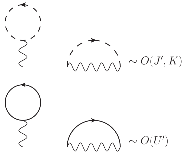
Figure 4: Typical Hartree-Fock diagrammatic contributions to the self-energy ${\bm{\Sigma}}^{HF}_{nm}$. The solid and dashed lines represent the $2\times 2$ single-particle excitation propagator ${\bf G}$ and the condensate propagator ${\bf C}$, respectively. The wavy lines denote the interactions $K,J^{\prime}$ or $U^{\prime}$, depending on which physical process of the Hamiltonian (18) is involved.

The equation of motion for the time-dependent condensate amplitude $a_{\alpha}(t)$ can be obtained by taking the upper left component of Eq. (47) and then dividing by $a_{\beta}^{*}(t^{\prime})$,

$$i\frac{\partial}{\partial t}a_{\alpha}=\left[E_{\alpha\gamma}+S^{HF}_{\alpha\gamma}(t)\right]a_{\gamma}(t)+W^{HF}_{\alpha\gamma}(t)a_{\gamma}^{*}(t).$$ (54)

Equations (48) and (49) for spectral and statistical propagators decouple in the BHF limit, it is therefore sufficient to consider only Eq. (49) in this case

$$i\tau_{3}\delta_{n\ell}\frac{\partial}{\partial t}{\bf F}_{\ell m}(t,t^{\prime})=\left[\epsilon_{n}\delta_{n\ell}\mathds{1}+{\bf\Sigma}^{HF}_{n\ell}(t)\right]{\bf F}_{\ell m}(t,t^{\prime}).$$ (55)

By taking the difference (or the sum) of Eq. (55) with its hermitian conjugate we obtain two equations

$$\begin{split}&i\left(\frac{\partial}{\partial t}\text{F}^{G}_{nm}(t,t^{\prime})+\frac{\partial}{\partial t^{\prime}}\text{F}^{G}_{nm}(t,t^{\prime})\right)=\\ &\left[\epsilon_{n}\delta_{n\ell}+\Sigma^{HF}_{n\ell}(t)\right]\text{F}^{G}_{\ell m}(t,t^{\prime})-\Omega^{HF}_{n\ell}(t)\text{F}^{F}_{\ell m}(t,t^{\prime})^{*}-\\ &\text{F}^{G}_{n\ell}(t,t^{\prime})\left[\epsilon_{m}\delta_{m\ell}+\Sigma^{HF}_{\ell m}(t^{\prime})\right]-\text{F}^{F}_{n\ell}(t,t^{\prime})\Omega^{HF}_{\ell m}(t^{\prime})^{*},\end{split}$$ (56)

and

$$\begin{split}&i\left(\frac{\partial}{\partial t}\text{F}^{F}_{nm}(t,t^{\prime})+\frac{\partial}{\partial t^{\prime}}\text{F}^{F}_{nm}(t,t^{\prime})\right)=\\ &\left[\varepsilon_{n}\delta_{n\ell}+\Sigma^{HF}_{n\ell}(t)\right]\text{F}^{F}_{\ell m}(t,t^{\prime})-\Omega^{HF}_{n\ell}(t)\text{F}^{G}_{\ell m}(t,t^{\prime})^{*}+\\ &\text{F}^{F}_{n\ell}(t,t^{\prime})\left[\varepsilon_{m}\delta_{m\ell}+\Sigma^{HF}_{\ell m}(t^{\prime})\right]+\text{F}^{G}_{n\ell}(t,t^{\prime})\Omega^{HF}_{\ell m}(t^{\prime})^{*}.\end{split}$$ (57)

The self-energies $\Sigma^{HF}_{nm}(t)$ and $\Omega^{HF}_{nm}(t)$ in these equations are given by

$$\Sigma^{HF}_{nm}(t) = K(N_{1}(t)+N_{2}(t))+J^{\prime}a_{1}^{*}(t)a_{2}(t)$$ (58)

$$+ J^{\prime}a_{2}^{*}(t)a_{1}(t)+2iU^{\prime}\sum_{s,\ell}\text{F}^{G}_{s\ell}(t,t),$$

$$\Omega^{HF}_{nm}(t) = \frac{K}{2}\sum_{\alpha=1}^{2}a_{\alpha}(t)a_{\alpha}(t)+J^{\prime}a_{1}(t)a_{2}(t)$$ (59)

$$+ iU^{\prime}\sum_{s,\ell}\text{F}^{F}_{s\ell}(t,t).$$

In order to get the final BHF equations we need to evaluate Eqs. (56) and (57) at equal times, as a result we obtain

$$\begin{split}i\frac{\partial}{\partial t}\text{F}^{G}_{nm}(t,t)&=\left[\varepsilon_{n}\delta_{n\ell}+\Sigma^{HF}_{n\ell}(t)\right]\text{F}^{G}_{\ell m}(t,t)\\ &-\text{F}^{G}_{n\ell}(t,t)\left[\varepsilon_{m}\delta_{m\ell}+\Sigma^{HF}_{\ell m}(t)\right]\\ &-\Omega^{HF}_{n\ell}(t)\text{F}^{F}_{\ell m}(t,t)^{*}-\text{F}^{F}_{n\ell}(t,t)\Omega^{HF}_{\ell m}(t)^{*},\end{split}$$ (60)

$$\begin{split}i\frac{\partial}{\partial t}\text{F}^{F}_{nm}(t,t)&=\left[\varepsilon_{n}\delta_{n\ell}+\Sigma^{HF}_{n\ell}(t)\right]\text{F}^{F}_{\ell m}(t,t)\\ &+\text{F}^{F}_{n\ell}(t,t)\left[\varepsilon_{m}\delta_{m\ell}+\Sigma^{HF}_{\ell m}(t)\right]\\ &-\Omega^{HF}_{n\ell}(t)\text{F}^{G}_{\ell m}(t,t)^{*}+\text{F}^{G}_{n\ell}(t,t)\Omega^{HF}_{\ell m}(t)^{*}.\end{split}$$ (61)

From Eq. (54) we get

$$\begin{split}i\frac{\partial}{\partial t}a_{1}(t)&=\left[\varepsilon_{0}+UN_{1}(t)+iK\sum_{n,m}\text{F}^{G}_{nm}(t,t)\right]a_{1}(t)\\ &-\left[J-iJ^{\prime}\sum_{n,m}\text{F}^{G}_{nm}(t,t)\right]a_{2}(t)\\ &+i\left[\frac{K}{2}a_{1}^{*}(t)+\frac{J^{\prime}}{2}a_{2}^{*}(t)\right]\sum_{n,m}\text{F}^{F}_{nm}(t,t)\end{split}$$ (62)

The equation for $a_{2}(t)$ is obtained from Eq.(62) by replacing $a_{1}$ by $a_{2}$ and visa versa. We solve differential Eqs. (60), (61) and (62) numerically for different parameters (22), and different initial conditions $z(0),\theta(0),N_{\textrm{tot}}=N_{1}(0)+N_{2}(0)$. We limit the number of levels which can be occupied by the QPs to $M=5$.

III.4 Collisions in Self-Consistent Second-Order Approximation

As we have mentioned, the BEC oscillations dynamically generate incoherent excitations (QPs), whose collisions, in turn, may lead to an ultimate thermalization of the system at some finite temperature $T$ controlled by $E_{BEC}(0)$. Although QP generation can be described within the first order BHF approximation, their collisions and eventual equilibration of the system can not. In this section we take into account all second order terms and derive integro-differential equations of motion, which capture the physics of thermalization. Typical second-order contributions to the quasiparticle self-energies are shown in Fig. 5. These second-order contributions will lead to a system of IPDE-s, which take into account "memory" effects which are crucial for eventual relaxation of the system.

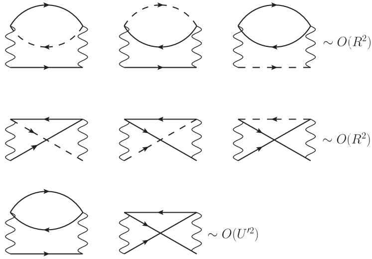
Figure 5: Typical second-order diagrammatic contributions to the QP self-energy ${\bm{\Sigma}}$ (27). The solid and dashed lines represent the $2\times 2$ single-particle excitation propagator ${\bf G}$ and the condensate propagator ${\bf C}$, respectively. The wavy lines denote the interactions $U,K,J^{\prime},U^{\prime}$ or $R$ from (22), depending on which physical processes of the Hamiltonian (18) are involved.

Specifically, we need to calculate the non-local self-energies $\gamma,{\bf\Gamma},{\bf\Pi}$ in the integral parts of Eqs. (47), (48) and (49). The self-energies are, as usual, matrices in the Bogoliubov space

$${\bf\gamma}_{\alpha\beta}(t,t^{\prime}) = \left(\begin{array}[]{cc}\gamma^{G}_{\alpha\beta}(t,t^{\prime})&\gamma^{F}_{\alpha\beta}(t,t^{\prime})\\ \gamma^{\overline{F}}_{\alpha\beta}(t,t^{\prime})&\gamma^{\overline{G}}_{\gamma\beta}(t,t^{\prime})\end{array}\right),$$ (65)

$${\bf\Gamma}_{nm}(t,t^{\prime}) = \left(\begin{array}[]{cc}\Gamma^{G}_{nm}(t,t^{\prime})&\Gamma^{F}_{nm}(t,t^{\prime})\\ \Gamma^{\overline{F}}_{nm}(t,t^{\prime})&\Gamma^{\overline{G}}_{nm}(t,t^{\prime})\end{array}\right),$$ (68)

$${\bf\Pi}_{nm}(t,t^{\prime}) = \left(\begin{array}[]{cc}\Pi^{G}_{nm}(t,t^{\prime})&\Pi^{F}_{nm}(t,t^{\prime})\\ \Pi^{\overline{F}}_{nm}(t,t^{\prime})&\Pi^{\overline{G}}_{nm}(t,t^{\prime})\end{array}\right).$$ (71)

We can now use the symmetry relations (44) and express the collisional self-energies in terms of only $\text{A}^{G},\text{A}^{F}$ and $\text{F}^{G},\text{F}^{F}$. We then obtain for $\gamma$ in (47)

$$\gamma_{\alpha\alpha^{\prime}}^{G}(t,t^{\prime})=R^{2}\sum_{nls}\sum_{n^{\prime}l^{\prime}s^{\prime}}\left(\text{F}_{nn^{\prime}}^{G}(t,t^{\prime})\left\{4\Lambda_{ss^{\prime}}^{\ell\ell^{\prime}}[\text{F},\text{F}^{*}](t,t^{\prime})\right.\right.$$

$$\left.+2\Lambda_{ss^{\prime}}^{\ell\ell^{\prime}}[\text{G},\text{G}^{*}](t,t^{\prime})\right\}$$

$$\left.+\text{A}_{nn^{\prime}}^{G}(t,t^{\prime})\left\{4\Xi_{ss^{\prime}}^{\ell\ell^{\prime}}[\text{F},\text{F}^{*}](t,t^{\prime})+2\Xi_{ss^{\prime}}^{\ell\ell^{\prime}}[\text{G},\text{G}^{*}](t,t^{\prime})\right\}\right)$$

$$\gamma_{\alpha\alpha^{\prime}}^{F}(t,t^{\prime})=R^{2}\sum_{nls}\sum_{n^{\prime}l^{\prime}s^{\prime}}\left(\text{F}_{nn^{\prime}}^{F}(t,t^{\prime})\left\{4\Lambda_{ss^{\prime}}^{\ell\ell^{\prime}}[\text{G},\text{G}^{*}](t,t^{\prime})\right.\right.$$

$$\left.+2\Lambda_{ss^{\prime}}^{\ell\ell^{\prime}}[\text{F},\text{F}^{*}](t,t^{\prime})\right\}$$

$$\left.+\text{A}_{nn^{\prime}}^{F}(t,t^{\prime})\left\{4\Xi_{ss^{\prime}}^{\ell\ell^{\prime}}[\text{G},\text{G}^{*}](t,t^{\prime})+2\Xi_{ss^{\prime}}^{\ell\ell^{\prime}}[\text{F},\text{F}^{*}](t,t^{\prime})\right\}\right).$$

In order to make the structure of our equations more transparent, we introduced the shorthand notations

$$\begin{split}\Lambda_{ss^{\prime}}^{\ell\ell^{\prime}}[\text{G},\text{F}](t,t^{\prime})&=\text{A}_{\ell\ell^{\prime}}^{G}(t,t^{\prime})\text{F}^{F}_{ss^{\prime}}(t,t^{\prime})\\ &+\text{F}_{\ell\ell^{\prime}}^{G}(t,t^{\prime})\text{A}^{F}_{ss^{\prime}}(t,t^{\prime}),\\ \Lambda_{ss^{\prime}}^{\ell\ell^{\prime}}[\text{G},\text{G}^{*}](t,t^{\prime})&=\text{A}_{\ell\ell^{\prime}}^{G}(t,t^{\prime})\text{F}^{G}_{ss^{\prime}}(t,t^{\prime})^{*}\\ &+\text{F}_{\ell\ell^{\prime}}^{G}(t,t^{\prime})\text{A}^{G}_{ss^{\prime}}(t,t^{\prime})^{*},\\ \Xi_{ss^{\prime}}^{\ell\ell^{\prime}}[\text{G},\text{F}](t,t^{\prime})&=\text{F}_{\ell\ell^{\prime}}^{G}(t,t^{\prime})\text{F}^{F}_{ss^{\prime}}(t,t^{\prime})\\ &-\frac{1}{4}\text{A}_{\ell\ell^{\prime}}^{G}(t,t^{\prime})\text{A}^{F}_{ss^{\prime}}(t,t^{\prime}),\\ \Xi_{ss^{\prime}}^{\ell\ell^{\prime}}[\text{G},\text{G}^{*}](t,t^{\prime})&=\text{F}_{\ell\ell^{\prime}}^{G}(t,t^{\prime})\text{F}^{G}_{ss^{\prime}}(t,t^{\prime})^{*}\\ &-\frac{1}{4}\text{A}_{\ell\ell^{\prime}}^{G}(t,t^{\prime})\text{A}^{G}_{ss^{\prime}}(t,t^{\prime})^{*},\end{split}$$ (73)

and so on. The remaining components of the self-energy $\gamma$ are related to $\gamma^{G}$ and $\gamma^{F}$ by the symmetry relations

$$\gamma^{G}(t,t^{\prime})^{*} = -\gamma^{\overline{G}}(t,t^{\prime})=\gamma^{G}(t^{\prime},t),$$

$$\gamma^{F}(t,t^{\prime})^{*} = -\gamma^{\overline{F}}(t,t^{\prime})=\gamma^{\overline{F}}(t^{\prime},t).$$ (74)

For the self-energy ${\bf\Gamma}$ in Eqs. (48) and (49) we get

$$\Gamma^{G}_{nn^{\prime}}(t,t^{\prime})=2iR^{2}\sum_{\alpha\ell s}\sum_{\alpha^{\prime}\ell^{\prime}s^{\prime}}\left(2a_{\alpha}^{*}(t)a_{\alpha^{\prime}}^{*}(t^{\prime})\Lambda_{ss^{\prime}}^{\ell\ell^{\prime}}[\text{G},\text{F}](t,t^{\prime})\right.$$

$$+a_{\alpha}^{*}(t)a_{\alpha^{\prime}}(t^{\prime})\Lambda_{ss^{\prime}}^{\ell\ell^{\prime}}[\text{G},\text{G}](t,t^{\prime})$$

$$-2a_{\alpha}(t)a_{\alpha^{\prime}}(t^{\prime})\Lambda_{ss^{\prime}}^{\ell\ell^{\prime}}[\text{F}^{*},\text{G}](t,t^{\prime})$$

$$-\left.2a_{\alpha}(t)a_{\alpha^{\prime}}^{*}(t^{\prime})\left\{\Lambda_{ss^{\prime}}^{\ell\ell^{\prime}}[\text{G},\text{G}^{*}](t,t^{\prime})+\Lambda_{ss^{\prime}}^{\ell\ell^{\prime}}[\text{F},\text{F}^{*}](t,t^{\prime})\right\}\right)$$

$$+(U^{\prime})^{2}\sum_{m\ell s}\sum_{m^{\prime}\ell^{\prime}s^{\prime}}\left(\text{F}^{G}_{mm^{\prime}}(t,t^{\prime})\left\{4\Lambda_{ss^{\prime}}^{\ell\ell^{\prime}}[\text{F},\text{F}^{*}](t,t^{\prime})\right.\right.$$

$$\left.+2\Lambda_{ss^{\prime}}^{\ell\ell^{\prime}}[\text{G},\text{G}^{*}](t,t^{\prime})\right\}$$

$$+\left.\text{A}^{G}_{mm^{\prime}}(t,t^{\prime})\left\{4\Xi_{ss^{\prime}}^{\ell\ell^{\prime}}[\text{F},\text{F}^{*}](t,t^{\prime})+2\Xi_{ss^{\prime}}^{\ell\ell^{\prime}}[\text{G},\text{G}^{*}](t,t^{\prime})\right\}\right)$$

and

$$\Gamma_{nn^{\prime}}^{F}(t,t^{\prime})=2iR^{2}\sum_{\alpha\ell s}\sum_{\alpha^{\prime}\ell^{\prime}s^{\prime}}\left(2a_{\alpha}^{*}(t)a_{\alpha^{\prime}}(t^{\prime})\Lambda_{ss^{\prime}}^{\ell\ell^{\prime}}[\text{G},\text{F}](t,t^{\prime})\right.$$

$$+a_{\alpha}^{*}(t)a_{\alpha^{\prime}}^{*}(t^{\prime})\Lambda_{ss^{\prime}}^{\ell\ell^{\prime}}[\text{F},\text{F}](t,t^{\prime})$$

$$-2a_{\alpha}(t)a_{\alpha^{\prime}}^{*}(t^{\prime})\Lambda_{ss^{\prime}}^{\ell\ell^{\prime}}[\text{G}^{*},\text{F}](t,t^{\prime})$$

$$-\left.2a_{\alpha}(t)a_{\alpha^{\prime}}(t^{\prime})\left\{\Lambda_{ss^{\prime}}^{\ell\ell^{\prime}}[\text{G},\text{G}^{*}](t,t^{\prime})+\Lambda_{ss^{\prime}}^{\ell\ell^{\prime}}[\text{F},\text{F}^{*}](t,t^{\prime})\right\}\right)$$

$$+(U^{\prime})^{2}\sum_{m\ell s}\sum_{m^{\prime}\ell^{\prime}s^{\prime}}\left(\text{F}^{F}_{mm^{\prime}}(t,t^{\prime})\left\{2\Lambda_{ss^{\prime}}^{\ell\ell^{\prime}}[\text{F},\text{F}^{*}](t,t^{\prime})\right.\right.$$

$$\left.+4\Lambda_{ss^{\prime}}^{\ell\ell^{\prime}}[\text{G},\text{G}^{*}](t,t^{\prime})\right\}$$

$$+\left.\text{A}^{F}_{mm^{\prime}}(t,t^{\prime})\left\{2\Xi_{ss^{\prime}}^{\ell\ell^{\prime}}[\text{F},\text{F}^{*}](t,t^{\prime})+4\Xi_{ss^{\prime}}^{\ell\ell^{\prime}}[\text{G},\text{G}^{*}](t,t^{\prime})\right\}\right).$$

While for the self-energy ${\bf\Pi}$ in Eq. (49) we have

$$\Pi^{G}_{nn^{\prime}}(t,t^{\prime})=2iR^{2}\sum_{\alpha\ell s}\sum_{\alpha^{\prime}\ell^{\prime}s^{\prime}}\left(2a_{\alpha}^{*}(t)a_{\alpha^{\prime}}^{*}(t^{\prime})\Xi_{ss^{\prime}}^{\ell\ell^{\prime}}[\text{G},\text{F}](t,t^{\prime})\right.$$

$$+a_{\alpha}^{*}(t)a_{\alpha^{\prime}}(t^{\prime})\Xi_{ss^{\prime}}^{\ell\ell^{\prime}}[\text{G},\text{G}](t,t^{\prime})$$

$$-2a_{\alpha}(t)a_{\alpha^{\prime}}(t^{\prime})\Xi_{ss^{\prime}}^{\ell\ell^{\prime}}[\text{F}^{*},\text{G}](t,t^{\prime})$$

$$-\left.2a_{\alpha}(t)a_{\alpha^{\prime}}^{*}(t^{\prime})\left\{\Xi_{ss^{\prime}}^{\ell\ell^{\prime}}[\text{G},\text{G}^{*}](t,t^{\prime})+\Xi_{ss^{\prime}}^{\ell\ell^{\prime}}[\text{F},\text{F}^{*}](t,t^{\prime})\right\}\right)$$

$$+(U^{\prime})^{2}\sum_{m\ell s}\sum_{m^{\prime}\ell^{\prime}s^{\prime}}\left(\text{F}^{G}_{mm^{\prime}}(t,t^{\prime})\left\{4\Xi_{ss^{\prime}}^{\ell\ell^{\prime}}[\text{F},\text{F}^{*}](t,t^{\prime})\right.\right.$$

$$\left.+2\Xi_{ss^{\prime}}^{\ell\ell^{\prime}}[\text{G},\text{G}^{*}](t,t^{\prime})\right\}$$

$$-\left.\frac{1}{2}\text{A}^{G}_{mm^{\prime}}(t,t^{\prime})\left\{2\Lambda_{ss^{\prime}}^{\ell\ell^{\prime}}[\text{F},\text{F}^{*}](t,t^{\prime})+\Lambda_{ss^{\prime}}^{\ell\ell^{\prime}}[\text{G},\text{G}^{*}](t,t^{\prime})\right\}\right)$$

and

$$\Pi_{nn^{\prime}}^{F}(t,t^{\prime})=2iR^{2}\sum_{\alpha\ell s}\sum_{\alpha^{\prime}\ell^{\prime}s^{\prime}}\left(2a_{\alpha}^{*}(t)a_{\alpha^{\prime}}(t^{\prime})\Xi_{ss^{\prime}}^{\ell\ell^{\prime}}[\text{G},\text{F}](t,t^{\prime})\right.$$

$$+a_{\alpha}^{*}(t)a_{\alpha^{\prime}}^{*}(t^{\prime})\Xi_{ss^{\prime}}^{\ell\ell^{\prime}}[\text{F},\text{F}](t,t^{\prime})$$

$$-2a_{\alpha}(t)a_{\alpha^{\prime}}^{*}(t^{\prime})\Xi_{ss^{\prime}}^{\ell\ell^{\prime}}[\text{G}^{*},\text{F}](t,t^{\prime})$$

$$-\left.2a_{\alpha}(t)a_{\alpha^{\prime}}(t^{\prime})\left\{\Xi_{ss^{\prime}}^{\ell\ell^{\prime}}[\text{G},\text{G}^{*}](t,t^{\prime})+\Xi_{ss^{\prime}}^{\ell\ell^{\prime}}[\text{F},\text{F}^{*}](t,t^{\prime})\right\}\right)$$

$$+(U^{\prime})^{2}\sum_{m\ell s}\sum_{m^{\prime}\ell^{\prime}s^{\prime}}\left(\text{F}^{F}_{mm^{\prime}}(t,t^{\prime})\left\{2\Xi_{ss^{\prime}}^{\ell\ell^{\prime}}[\text{F},\text{F}^{*}](t,t^{\prime})\right.\right.$$

$$\left.+4\Xi_{ss^{\prime}}^{\ell\ell^{\prime}}[\text{G},\text{G}^{*}](t,t^{\prime})\right\}$$

$$-\left.\frac{1}{2}\text{A}^{F}_{mm^{\prime}}(t,t^{\prime})\left\{\Lambda_{ss^{\prime}}^{\ell\ell^{\prime}}[\text{F},\text{F}^{*}](t,t^{\prime})+2\Lambda_{ss^{\prime}}^{\ell\ell^{\prime}}[\text{G},\text{G}^{*}](t,t^{\prime})\right\}\right).$$

The following symmetry relations apply for the collisional self-energies

$$\Gamma^{G}(t,t^{\prime})^{*} = -\Gamma^{\overline{G}}(t,t^{\prime})=\Gamma^{G}(t^{\prime},t),$$

$$\Gamma^{F}(t,t^{\prime})^{*} = -\Gamma^{\overline{F}}(t,t^{\prime})=\Gamma^{\overline{F}}(t^{\prime},t),$$

$$\Pi^{G}(t,t^{\prime})^{*} = -\Pi^{\overline{G}}(t,t^{\prime})=-\Pi^{G}(t^{\prime},t),$$

$$\Pi^{F}(t,t^{\prime})^{*} = -\Pi^{\overline{F}}(t,t^{\prime})=-\Pi^{\overline{F}}(t^{\prime},t).$$ (79)

The final equations of motion in the collisional case can be then written as follows: for the spectral function

$$i\frac{\partial}{\partial t}\text{A}^{G}_{nm}(t,t^{\prime})=(\varepsilon_{n}\delta_{n\ell}+\Sigma^{HF}_{n\ell})\text{A}^{G}_{\ell m}(t,t^{\prime})$$

$$-\Omega_{n\ell}^{HF}(t)(\text{A}^{F}_{\ell m}(t,t^{\prime}))^{*}$$

$$-i\int_{t^{\prime}}^{t}d{\overline{t}}\left[\Gamma^{G}_{n\ell}(t,{\overline{t}})\text{A}^{G}_{\ell m}({\overline{t},t^{\prime}})+\Gamma^{F}_{n\ell}(t,{\overline{t}})\text{A}^{\overline{F}}_{\ell m}({\overline{t}},t^{\prime})\right]$$

$$i\frac{\partial}{\partial t}\text{A}^{F}_{nm}(t,t^{\prime})=(\varepsilon_{n}\delta_{n\ell}+\Sigma^{HF}_{n\ell})\text{A}^{F}_{\ell m}(t,t^{\prime})$$

$$-\Omega_{n\ell}^{HF}(t)(\text{A}^{G}_{\ell m}(t,t^{\prime}))^{*}$$

$$-i\int_{t^{\prime}}^{t}d{\overline{t}}\left[\Gamma^{G}_{n\ell}(t,{\overline{t}})\text{A}^{F}_{\ell m}({\overline{t},t^{\prime}})+\Gamma^{F}_{n\ell}(t,{\overline{t}})\text{A}^{\overline{G}}_{\ell m}({\overline{t}},t^{\prime})\right].$$ (80)

For the statistical function we get

$$i\frac{\partial}{\partial t}\text{F}^{G}_{nm}(t,t^{\prime})=(\varepsilon_{n}\delta_{n\ell}+\Sigma^{HF}_{n\ell})\text{F}^{G}_{\ell m}(t,t^{\prime})$$

$$-\Omega_{n\ell}^{HF}(t)(\text{F}^{F}_{\ell m}(t,t^{\prime}))^{*}$$

$$-i\int_{0}^{t}d{\overline{t}}\left[\Gamma^{G}_{n\ell}(t,{\overline{t}})\text{F}^{G}_{\ell m}({\overline{t},t^{\prime}})+\Gamma^{F}_{n\ell}(t,{\overline{t}})\text{F}^{\overline{F}}_{\ell m}({\overline{t}},t^{\prime})\right]$$

$$+i\int_{0}^{t}d{\overline{t}}\left[\Pi^{G}_{n\ell}(t,{\overline{t}})\text{A}^{G}_{\ell m}({\overline{t},t^{\prime}})+\Pi^{F}_{n\ell}(t,{\overline{t}})\text{A}^{\overline{F}}_{\ell m}({\overline{t}},t^{\prime})\right]$$

$$i\frac{\partial}{\partial t}\text{F}^{F}_{nm}(t,t^{\prime})=(\varepsilon_{n}\delta_{n\ell}+\Sigma^{HF}_{n\ell})\text{F}^{F}_{\ell m}(t,t^{\prime})$$

$$-\Omega_{n\ell}^{HF}(t)(\text{F}^{G}_{\ell m}(t,t^{\prime}))^{*}$$

$$-i\int_{0}^{t}d{\overline{t}}\left[\Gamma^{G}_{n\ell}(t,{\overline{t}})\text{F}^{F}_{\ell m}({\overline{t},t^{\prime}})+\Gamma^{F}_{n\ell}(t,{\overline{t}})\text{F}^{\overline{G}}_{\ell m}({\overline{t}},t^{\prime})\right]$$

$$+i\int_{0}^{t}d{\overline{t}}\left[\Pi^{G}_{n\ell}(t,{\overline{t}})\text{A}^{F}_{\ell m}({\overline{t},t^{\prime}})+\Pi^{F}_{n\ell}(t,{\overline{t}})\text{A}^{\overline{G}}_{\ell m}({\overline{t}},t^{\prime})\right].$$ (81)

And, finally, for the condensate amplitudes we have

$$i\frac{\partial}{\partial t}a_{\alpha}(t)=-Ja_{\beta\neq\alpha}(t)+S_{\alpha\beta}^{HF}a_{\beta}(t)+W_{\alpha\beta}^{HF}a_{\beta}^{*}(t)$$

$$-i\int_{0}^{t}d{\overline{t}}\left[\gamma_{\alpha\beta}^{G}(t,{\overline{t}})a_{\beta}({\overline{t}})+\gamma^{F}_{\alpha\beta}(t,{\overline{t}})a^{*}_{\beta}({\overline{t}})\right],$$ (82)

with the self-energies specified at the beginning of the section. We also used the symmetry relations (44) in order to express all quantities appearing in the equations of motion with the later time argument on the left side. This implies that we only need to know the solution of the previous steps while evolving the equations in time (this is beneficial for the numerical implementation - see Appendix A). The integro-differential equations (80), (81) and (82) are then solved for different values of parameters (22) and different initial values $z(0),\theta(0),N_{\textrm{tot}}=N_{1}(0)+N_{2}(0)$.

The kinetic equations (80), (81) and (82) are derived here for the case of two weakly-coupled trapped condensates, however, since our formalism is quite general, they can be easily extended to the case of several weakly coupled condensates and to optical lattices, where non-equilibrium dynamics in the weakly interacting regime can be analysed in detail Mauro2017 .

IV Quasiparticle Creation and Thermalization Dynamics

IV.1 Results within Bogoliubov-Hartree-Fock Approximation

In this section we present numerical solutions of Eqs. (60), (61) and (62) for total number of particles $N_{\textrm{tot}}=500000$, level spacing $\Delta$, interactions $U,\,U^{\prime},\,K,\,J^{\prime}$. As initial conditions we take all particles in the condensate, $N_{1}(0)+N_{2}(0)=N_{\textrm{tot}}$, with population imbalance $z(0)$ and phase difference $\theta(0)$ between the BECs in the two wells at time $t=0$, that is,

$$a_{\alpha}(0) = \sqrt{N_{\alpha}(0)}e^{i\theta_{\alpha}(0)},\qquad\alpha=1,2$$

$$\text{F}^{G}_{nm}(0,0) = -\frac{i}{2}\delta_{nm}$$ (83)

$$\text{F}^{F}_{nm}(0,0) = 0.$$

Note that the large particle number we chose is at least two orders of magnitude larger then the number of atoms in realistic experiments Albiez2005 ; Thywissen2011 . We did it in order to make the distinction between BEC and incoherent excitation especially pronounced.

It is convenient to express all energies in units of the bare Josephson coupling $J$: $u=UN_{\textrm{tot}}/J$, $u^{\prime}=U^{\prime}N_{\textrm{tot}}/J$, $k=KN_{\textrm{tot}}/J$, $j^{\prime}=J^{\prime}N_{\textrm{tot}}/J$, $r=RN_{\textrm{tot}}/J$, whereas time $t$ is given in units of $1/J$. We emphasize that in general these parameters are determined by the trap and by the scattering length of the atoms in the trap (see Eqs. (22)). In this work we choose certain characteristic values in order to demonstrate the typical thermalization dynamics in the presence of quasiparticles. We calculate the time dependence of the condensate population imbalance $z(t)$, the phase difference $\theta(t)$, the QP occupation numbers $n_{m}(t)$ in the excited trap states, $m=1,2,..,5$, and the total occupation number

$$n_{\textrm{tot}}(t)=\sum_{m=1}^{5}n_{m}(t)=-\sum_{m=1}^{5}\left[\text{Im}\text{F}_{mm}^{G}(t,t)-\frac{1}{2}\right].$$ (84)

The QP occupation numbers are normalized by the total number of particles $N_{\textrm{tot}}$, which is conserved.

Our main finding in the BHF regime is that there exists a characteristic time scale $\tau_{c}$ associated with the creation of incoherent excitations (QPs) out of the condensate. When $J^{\prime}=K=0$, this time scale is infinite, and the system performs undamped Josephson oscillations, described by the semiclassical two-mode approximation Smerzi1997 . For non-zero interaction parameters, however, a qualitatively different dynamics sets in at the characteristic time $\tau_{c}$. At this time, QPs get excited, and the dynamics becomes dominated by fast QP Rabi oscillations between the discrete trap levels, which in turn drive the BEC oscillations Mauro2009 . We note that after the time $\tau_{c}$ inelastic QP collisions will become important and will be taken into account in section IV.2. The collisionless regime that exists up to $\tau_{c}$ and, therefore, the time scale $\tau_{c}$ itself can be described by the BHF approximation.

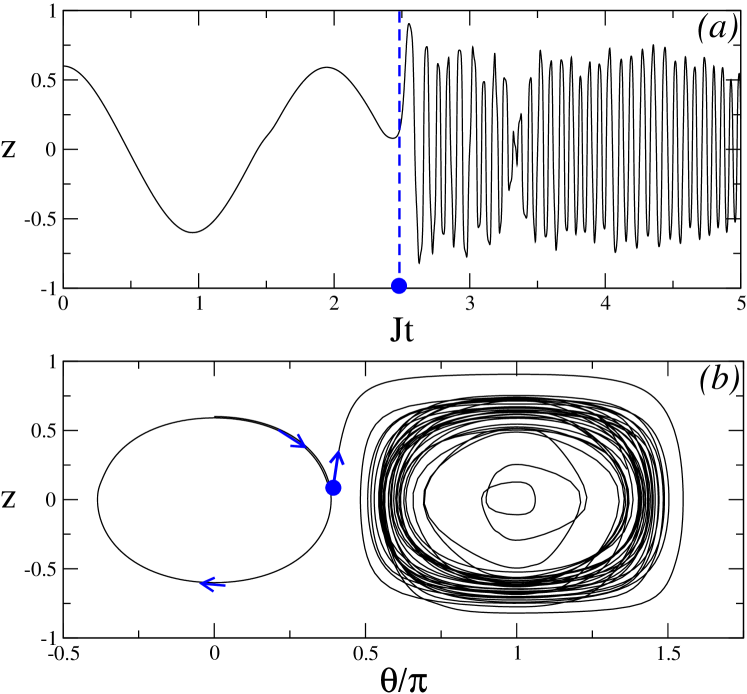
Figure 6: (a) Time-dependent population imbalance $z(t)$ and (b) phase space portrait for $\Delta=20,u=u^{\prime}=5,j^{\prime}=60,k=0$, and initial conditions $z(0)=0.6,\theta(0)=0$. The characteristic time scale $\tau_{c}$ is marked by the dashed vertical line, and $\tau_{c}$ is shown by the thick dot in both panels. The arrows indicate the clockwise direction of time evolution along the phase space trajectory.

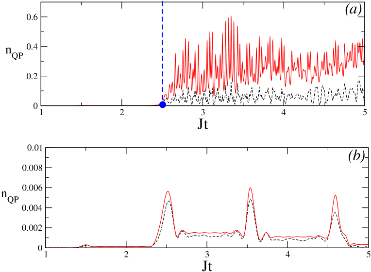
Figure 7: QP occupation numbers $n_{\text{QP}}$ (a) for the same parameters as in Fig. 6, (b) for the parameters as in Fig. 8. The dashed, black lines represent the QP occupation number of the first QP level: $n_{1}(t)$, while the solid, red lines correspond to the sum of all five levels $n_{\textrm{tot}}(t)$ (84). In (a) the dashed vertical line marks the onset of the QP dominated regime at $t=\tau_{c}$. In (b) $\tau_{c}$ is not identifiable.

In Fig. 6 we show how the QP creation sets in for a certain choice of the parameters in Eq. (22). In Fig. 6 (a) the commencement of the QP-dominated dynamics is indicated by the vertical dashed line, and $\tau_{c}$ by a thick dot. For $t<\tau_{c}$ the junction exhibits undamped Josephson oscillations with a frequency $\omega_{J}$ which can be estimated from the two-mode approximation as $\omega_{J}\approx 2J\sqrt{1+u/2}$ Smerzi1997 . At $t>\tau_{c}$ a substantial amount of QPs is abruptly created as seen in Fig. 7(a), and fast Rabi oscillations between the QP levels govern the dynamics.

It seems surprising at first sight that for a discrete spectrum $\tau_{c}$ can be non-zero. It means that QPs are not excited immediately, even though the initial state with $z(0)\neq 0$ is a highly excited state with a macroscopic excitation energy $E_{BEC}(0)$, sufficient to excite QPs. $E_{BEC}(0)$ is proportional to $z^{2}(0)N_{\textrm{tot}}J$, as derived in the next section IV.2. The reason is that the condensate oscillations act as a periodic perturbation with frequency $\omega_{J}$ on the QP subsystem. Therefore, for $\omega_{J}<\Delta_{\textrm{eff}}$ (where $\Delta_{\textrm{eff}}$ is the effective level spacing, renormalized by all interactions) QPs cannot be excited in low order time-dependent perturbation theory. QP excitations are possible only in higher orders which is a highly non-linear process and leads to the abrupt creation of QPs at $t=\tau_{c}$. For $t>\tau_{c}$, QP collisions are expected to ultimately thermalize the system, as described in section IV.2.

Figure 8: (a) Time-dependent population imbalance $z(t)$ and (b) phase space portrait for $\Delta=20,u=u^{\prime}=5,j^{\prime}=60,k=0.38$, and initial conditions $z(0)=0.6,\theta(0)=0$. $\tau_{c}$ is beyond the observation time in this case.

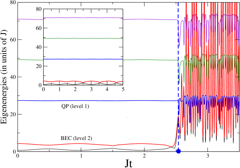
Figure 9: Renormalized single-particle levels of Hamiltonian (18) in BHF approximation for the parameters of Fig. 6: $\Delta=20,u=u^{\prime}=5,j^{\prime}=60,k=0$. The onset of the QP-dominated regime is indicated by the dashed, vertical line, and $\tau_{c}$ by the thick dot. The two lowest levels are the condensate levels (black and red), the first QP levels is marked as "level 1" (in blue). In the inset the instantaneous eigenenergies for the parameter set of Fig. 8 are shown. $\tau_{c}$ is unobservably large in this case.

Another remarkable phenomenon associated with the QP dynamics is that at $\tau_{c}$ that Josephson junction undergoes a $0-\pi$ transition, as can be seen from the phase space portrait in Fig. 6(b). Prior to $\tau_{c}$, the phase difference oscillates around $\theta(0)=0$, whereas for $t>\tau_{c}$ it oscillates around $\pi$. This behaviour can be understood recalling the analogy to a driven oscillator. While for $t<\tau_{c}$ the Josephson junction oscillates at its natural frequency $\omega_{J}$, for $t>\tau_{c}$ it is driven by the QP Rabi oscillations with frequencies $\omega_{R}\approx\Delta_{\textrm{eff}}>>\omega_{J}$ far above its resonance frequency and, thus, has a phase shift of $\pi$ with respect to the QP density as a driving force. The $0-\pi$ transition should be detectable in phase sensitive experiments Albiez2005 when QPs are excited.

The time scale $\tau_{c}$ depends strongly on the parameters of Eq. (22). Consequently, it is sensitive to details of the experimental setup, which can be realized in very dissimilar ways Albiez2005 ; Thywissen2011 ; Lappe2017 . In Fig. 8 we have chosen a different value of the BEC-QP coupling $k$, which results in a drastic suppression of QPs and therefore their negligible effect on the junction dynamics. In this case the Bose Josephson junction is well described within the semiclassical two-mode approximation Smerzi1997 , although a small density of incoherent excitations may be excited intermediately. Such a low QP density decays again, as shown in Fig. 7(b), and is not sufficient to induce fast Rabi oscillations or a $0-\pi$ transition, see Fig8(b).

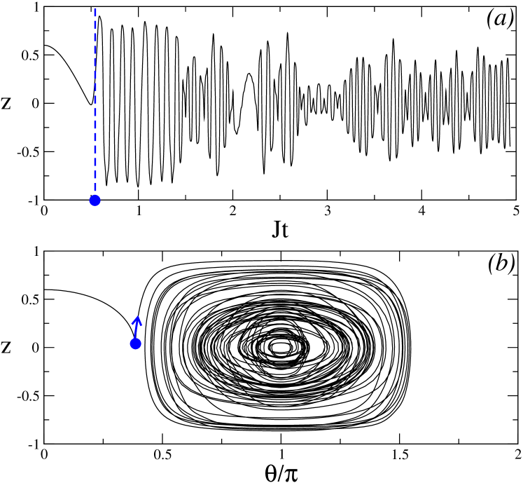
Figure 10: (a) Time-dependent population imbalance $z(t)$ and (b) phase space portrait for $\Delta=15,u=u^{\prime}=5,j^{\prime}=60,k=0$, and initial conditions $z(0)=0.6,\theta(0)=0$. The characteristic time scale $\tau_{c}$ is marked by the dashed vertical line, and $\tau_{c}$ is shown by the thick dot in both figures. The arrow indicates the direction of the time evolution along the phase space tranjectory.

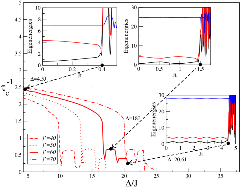
Figure 11: Dependence of the inverse characteristic time $\tau_{c}^{-1}$ on the interlevel spacing $\Delta$ for $z(0)=0.6,\theta(0)=0$ and k=0 for four values of the QP-assisted tunneling $j^{\prime}$. For three values of $\tau_{c}$ from the $j^{\prime}=60$ curve the time dependence of the energy levels are shown in the three insets as marked. The excitation of QPs is related to the level crossing discussed in the text.

In order to get a better understanding of the reasons of the abrupt QP generation, we analyzed the instantaneous single-particle levels of the Hamiltonian (18) in Bogoliubov-Hartree-Fock approximation, shown in Fig. 9 Mauro2015 . It turns out that the rapid QP production sets in when one of the condensate levels (BEC level 2 in Fig. 9) crosses or comes close to the first QP level ("QP level 1" in Fig. 9). In the case of negligible QP generation (Fig. 8) the levels never cross, as seen in the inset of Fig. 9. In view of the afore-mentioned physics it is clear that reducing interlevel spacing should accelerate QP production. This indeed happens and is demonstrated in Fig. 10. We reduce $\Delta$ by 25 $\%$, and as a result $\tau_{c}$ decreases by about 80 $\%$ compared to Fig. 6. However, an analytical parameter dependence of $\tau_{c}$ is difficult to obtain, since the transition to the QP-dominated regime is controlled by highly non-linear processes. Thus, a systematic numerical study of the inverse characteristic time $\tau_{c}^{-1}$ versus $\Delta$ for different $j^{\prime}$-s and fixed initial conditions is presented in Fig. 11. As expected, $\tau_{c}^{-1}$ generally decreases with increasing $\Delta$, but not in a monotonic way. Namely, one can distinguish two regimes of qualitatively different behavior of $1/\tau_{c}$, separated by the oscillation period $T_{12}$ of the condensate levels $\alpha=1,2$ for $t<\tau_{c}$: For $1/\tau_{c}>1/T_{12}$, $\tau_{c}$ depends on $\Delta$ in a continuous way, while for $1/\tau_{c}<1/T_{12}$ it jumps between certain discrete or plateau values. This happens because as long as $\tau_{c}$ is smaller than $T_{12}$, the condensates cannot perform a full Josephson oscillation before QPs get excited. As a result the BEC dynamics cannot be considered a periodic perturbation on the QP system, and any value of $\tau_{c}$ is possible, thus increasing continuously with $\Delta$. For larger $\Delta$, $\tau_{c}$ becomes larger than $T_{12}$, and $\tau_{c}$ takes on prefered plateau values which are related to the times when the condensate levels cross or come very close to each other and the first QP level (see insets of Fig. 11). The detailed discussion of this physics and the dependence of $\tau_{c}$ on the parameter $k$ can be found in Mauro2015 .

Finally, we comment on the self-trapped case. This regime of macroscopic self-trapping (ST) with a finite time average $\langle z(t)\rangle\neq 0$ and an unbounded phase difference $\theta(t)$ was predicted in Ref. Smerzi1997 and verified experimentally in Ref. Albiez2005 . In the preceding discussion we considered the initially delocalized regime with $\langle z(t)\rangle=0$ and oscillating $\theta(t)$. For the ST case the non-equilibrium dynamics is very similar to the delocalized case Mauro2015 . However, the values of $\Delta$ for which the QP creation time $\tau_{c}$ approaches zero are substantially greater due to the substantially greater BEC oscillation frequencies. It means that in the ST case the system is much easier to drive into the QP-dominated regime. The initial ST is always destroyed by the QP dynamics, see Fig. 12. For the initially self-trapped case we show the population imbalance dynamics only, because all other results are very similar to the delocalized case Mauro2015 . We note also, that first principle calculations on level energies and coupling constants, based on trap wave functions for realistic traps of the experiments of Ref. [34] and [36] are in preparation and will shed light on the precise mechanism of quasi-particle creation.

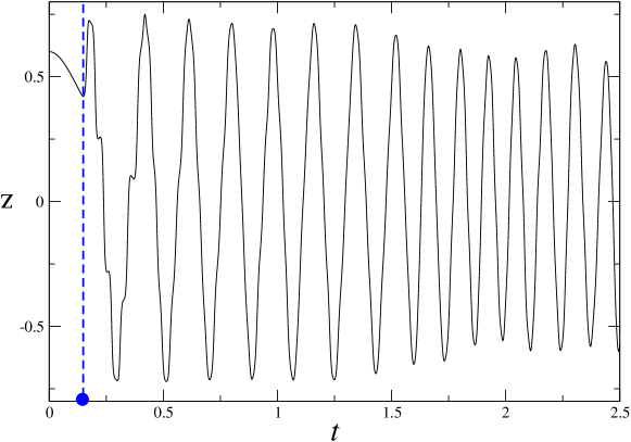
Figure 12: Time-dependent population imbalance in the initially self-trapped case $z(0)=0.6$, $\theta(0)=0$, $\Delta=20,u=u^{\prime}=22,j^{\prime}=60,k=10$. The characteristic time scale $\tau_{c}$ is marked by the dashed vertical line, and $\tau_{c}$ is shown by the thick dot.

IV.2 Thermalization by Quasiparticle Collisions

We demonstrate how the physics discussed in the previous section IV.1 is modified by inclusion of QP inelastic collisions (all second-order processes). We self-consistently solve Eqs. (80), (81) and (82) (for numerical details see Appendix A) for initially delocalized junctions.

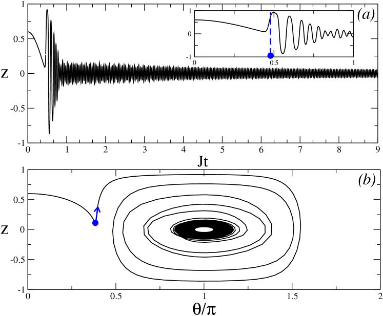
Figure 13: Time-dependent population imbalance $z(t)$ (a) and phase space portrait (b) for $\Delta=10,u=u^{\prime}=5,j^{\prime}=60,k=0,r=600$, and initial conditions $z(0)=0.6,\theta(0)=0$. The characteristic time scale $\tau_{c}$ is marked by the dashed vertical line in the inset, and $\tau_{c}$ is marked by thick dots. The arrow indicates direction of the time evolution along the phase trajectory after $\tau_{c}$.

We identify three different regimes and three time scales associated with the non-equlibrium dynamics of the Bose Josephson junction (see also Fig. 2). The regimes are the following.

1. Semiclassical regime for $0\leq t\leq\tau_{c}$.

   QPs are not excited, or their number is negligible, so that the BEC oscillations are undamped and well described within the two-mode approximation Smerzi1997 .

2. Strong coupling regime for $\tau_{c}<t<\tau_{f}$.

   As we know from section IV.1, the time $\tau_{c}\geq 0$ marks the onset of the QP dominated regime. Incoherent excitations are induced in an avalanche fashion due to a dynamically generated parametric resonance between the Josephson frequency and QP excitation energies, as shown below. The BEC and the QP subsystems are strongly coupled. This leads to a fast depletion as well as strong damping of the condensate amplitudes Anna2016 ; Yukalov2008 .

3. Weak coupling or hydrodynamic regime for $t>\tau_{f}$.

   At the "freeze-out" time $t=\tau_{f}>\tau_{c}$ the final number of excitations allowed by total energy conservation is reached. This results in an effective decoupling of the QP subsystem from the BEC oscillations and a near conservation of the total QP number. Because of this approximate conservation law, the system enters into a quasi-hydrodynamic regime which is characterized by exponential relaxation to thermodynamic equilibrium with a slow relaxation time $\tau_{th}>\tau_{f}$. The QP subsystem acts as a grand canonical reservoir for the BEC subsystem and vice versa. Remarkably, we observe that the thermalization times $\tau_{th}$ for the BEC and for the QP subsystems may be different (see below, Fig. 16).

We now illustrate this intricate non-equilibrium dynamics with our numerical results. In Fig. 13 we show an example of the population imbalance damping, and a phase portrait corresponding to the relaxation. We see that the $0-\pi$ transition survives and that the amplitude of the phase oscillations becomes smaller as one evolves in time, as expected. In Fig. 14 we compare QP occupation numbers calculated in the first-order approximation Fig. 14(a), and in full second-order Fig. Fig. 14(b). We see that compared to BHF the oscillations are strongly damped, although the average QP number can be even greater in the collisional regime. Three different regimes (semiclassical, strong coupling and weak coupling) are clearly distinguishable in Fig. 14.

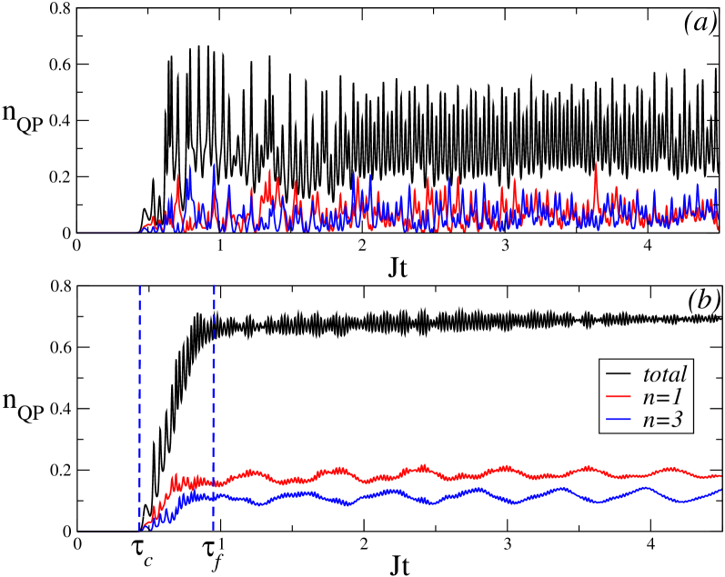
Figure 14: Time-dependent QP occupation numbers for the parameters as in Fig. 13 ($\Delta=10,u=u^{\prime}=5,j^{\prime}=60,k=0$) in (a) Bogoliubov-Hartree-Fock approximation, (b) second-order approximation including inelastic collisions ($r=300$). Red lines correspond to the occupation of the lowest QP level $n_{1}$, blue lines to the occupation of the third QP level $n_{3}$, and the black lines represent the occupation numbers summed over all 5 levels $n_{\textrm{tot}}$. Dashed vertical lines mark the time scales $\tau_{c}$ and $\tau_{f}$ discussed at the beginning of section IV.2.

Figure 15: Time-dependent population imbalance for $z(0)=0.6$, $\theta(0)=0$, $\Delta=9,u=u^{\prime}=5,j^{\prime}=40,k=0,r=300$. The inset shows small oscillations remaining in the long time limit.

To understand the origin of this behavior, we now consider a similar junction in more detail Anna2016 (see Fig. 15 for parameter values). In Fig. 16 we present logarithmic plots of (a) deviation of the running mean value $n_{\textrm{avg}}(t)$ of $n_{\textrm{tot}}(t)$ from its final value $n_{\textrm{avg}}(\infty)$; (b) $\Delta n(t)=n_{\textrm{tot}}(t)-n_{\textrm{avg}}(t)$, and (c) condensate population imbalance $z(t)$. All three logarithmic plots demonstrate the sharp crossover at $t=\tau_{f}$ from the strong to the weak coupling regimes and slow exponential relaxation for $t>\tau_{f}$.

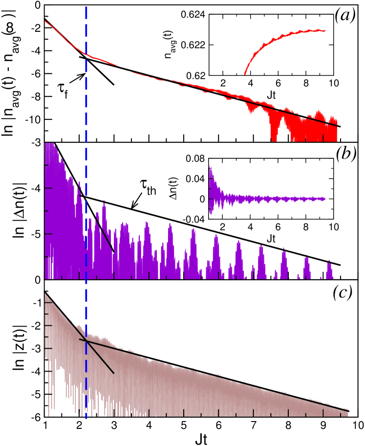
Figure 16: Logarithmic plots of the relaxation behavior of the QP subsystem (a) and (b), and of the BEC population imbalance (c) for the same parameters as in Fig. 15. The dashed vertical line marks the freeze-out time $\tau_{f}$. The thin, black lines are guides to the eye. The insets show the respective linear plots, for illustration. Anna2016 Copyright 2016 by the American Physical Society.

The physics behind the sharp crossover and the scale $\tau_{f}$ can be deduced from a spectral analysis of the non-equilibrium problem. We introduce the standard Wigner “center-of motion” (CoM) time $t=(t_{1}+t_{2})/2$ and difference time $\tau=(t_{1}-t_{2})$ and Fourier-transform the two-time Green’s functions $\text{A}^{G}(t_{1},t_{2})=\sum_{n}\text{A}_{nn}^{G}(t_{1},t_{2})$ and $\text{F}^{G}(t_{1},t_{2})=\sum_{n}\text{F}_{nn}^{G}(t_{1},t_{2})$ with respect to $\tau$. Note that away from equilibrium the Fourier-transformed functions are in general complex. We choose as the zero of the energy scale the renormalized energy $\tilde{\varepsilon}_{0}$ of the BEC in the long-time limit after the stationary state has been reached. In particular, this implies that the chemical potential in this final state is $\mu=0$. In Fig. 17 (a) and (b) we plot the frequency-dependent absolute values of $\text{A}^{G}(\omega,t)\equiv\text{A}(\omega)$ and $\text{F}^{G}(\omega,t)\equiv\text{F}(\omega)$ in the long-time regime, $t=9.01/J>\tau_{f}$. As expected, the spectra exhibit five nearly Lorentzian peaks corresponding to the renormalized QP levels. They mark the Rabi oscillation frequencies of the non-equilibrium QP system. The wiggly modulations of the Lorentzian peaks are due to a limited resolution of the Fourier transform Anna2016 . Fig. 17 (c) displays the power spectra of the BEC population imbalance $z(t)$, Fourier transformed with respect to $t$ for $\tau_{c}<t<\tau_{f}$ (red curve) and for $t>\tau_{f}$ (blue curve), respectively.

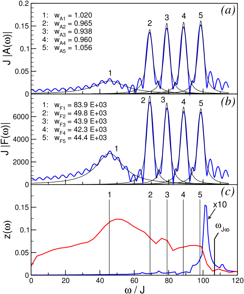
Figure 17: Absolute values of (a) spectral and (b) statistical functions, Fourier-transformed with respect to $\tau=(t_{1}-t_{2})$ for a fixed value of $t=(t_{1}+t_{2})/2=9.01/J$. The thin, black lines represent Lorentzian fits. The weights w of each of the five Lorentzians are shown in the insets. In (c) the power spectrum $z(\omega)$ of the BEC population imbalance is shown for $\tau_{c}\lesssim t\lesssim\tau_{f}$ (red line) and for $t>\tau_{f}$ (blue line). The vertical lines indicate renormalized QP energies. $\omega_{J\infty}$ is the Josephson frequency estimated for the quasi-hydrodynamic regime for $t>\tau_{f}$. Anna2016 Copyright 2016 by the American Physical Society.

The remarkable feature seen in Fig. 17 is that in the strong coupling regime, the condensate oscillation spectrum overlaps strongly with the QP spectrum $|\text{A}(\omega)|$ and has maxima approximately at renormalized Rabi frequencies. This is an indication of a dynamically generated parametric resonance which leads to an abrupt, "inflationary" QP creation. Very different behaviour is observed in the third regime (weak coupling regime). The BEC spectrum consists of essentially one sharp (compared to the broad spectrum in the strong coupling regime) peak, which has negligible overlap with the QP spectrum. Moreover, this peak is close to the eigenfrequency of the non-driven Josephson junction, which is $\omega_{J\infty}\approx 2J_{\textrm{eff}}\sqrt{1+uJ/(2J_{\textrm{eff}})}$, with $J_{\textrm{eff}}=J+n_{\textrm{tot}}(t\rightarrow\infty)J^{\prime}$ the QP-renormalized effective Josephson coupling Smerzi1997 ; Anna2016 . This manifests that the BEC performs essentially free, non-driven Josephson oscillations, i.e., the BEC and the QP subsystems are effectively decoupled in this final regime.

The emergence of the weak coupling regime can be understood from energy conservation arguments. The energy of the condensate subsystem can be calculated as the expectation value of the coherent parts of the Hamiltonian only, $H_{coh}$ and $H_{J}$. Hence, the general expression for the BEC energy in these regimes is,

$$E_{BEC} = \sum_{\alpha=1,2}\left[\varepsilon_{0}(N_{\alpha})+\frac{U}{2}(N_{\alpha}-1)N_{\alpha}\right]$$ (85)

$$- 2J\sqrt{N_{1}N_{2}}-3J^{\prime}N_{qp}\sqrt{N_{1}N_{2}}$$

where $N_{qp}$ is the particle number in the QP subsystem. $N_{1}$, $N_{2}$ and $N_{qp}$ can be expressed in terms of the total particle number $N$, the total condensate number $N_{c}$, and the population imbalance $z$ as

$$N_{1}+N_{2}=N_{c}\,,\qquad N_{1}-N_{2}=zN_{c}\,,\qquad N_{c}+N_{qp}=N\ .$$

Inserting this in Eq. (85), the BEC energy reads in terms of the reduced interaction constants $u$, $j^{\prime}$, and the condensate fraction $f=N_{c}/N$ as

$$E_{BEC} = \varepsilon_{0}fN+\left[\frac{u}{4}f\left(f-\frac{2}{N}\right)+\frac{u}{4}z^{2}f^{2}\right.$$

$$- \left.f\left(1-\frac{3}{2}j^{\prime}(1-f)\right)\sqrt{1-z^{2}}\right]NJ\ .$$

Hence, the initial-state energy at $t=0$, i.e., for $\varepsilon_{0}=0$, $f=1$, and $z=z(0)=z_{0}$, reads,

$$E_{BEC}(0)=\frac{u}{4}\left[(1+z_{0}^{2}-2/N)-\sqrt{1-z_{0}^{2}}\right]NJ\ .$$ (87)

The final-state energy for $t\to\infty$, where $\varepsilon_{0}=\varepsilon_{0}(\infty)\neq 0$ (renormalized by QP interactions), $f=f_{\infty}<1$ (finite, but decoupled QP population), and $z=0$ (BEC oscillations damped out), reads,

$$E_{BEC}(\infty) = \left[f_{\infty}\frac{\varepsilon_{0}(\infty)}{J}+\frac{u}{4}f_{\infty}\left(f_{\infty}-\frac{2}{N}\right)\right.$$

$$- \left.f_{\infty}\left(1+\frac{3}{2}j^{\prime}(1-f_{\infty})\right)\right]NJ\ .$$

The final-state parameters $\varepsilon_{0}(\infty)$ and $f_{\infty}$ can be obtained from the numerical solutions of Eqs. (80), (81) and (82).

The energy difference $\Delta E_{BEC}=E_{BEC}(0)-E_{BEC}(\infty)$ is in fact the maximum energy that can be provided to the QP subsystem by the condensate subsystem. Therefore, the energy of the QP subsystem $E_{QP}(t)$ initially increases but eventually saturates once the maximum is reached. This happens for $t>\tau_{f}$, and the number of QPs stays approximately constant thereafter. Our numerical computations show that indeed the maximum is attained at $t\approx\tau_{f}$. It means that for $t>\tau_{f}$ both $n_{\textrm{tot}}(t)$ and $E_{QP}(t)$ become approximately conserved in the grand canonical sense (particle and energy exchange between the subsystems are allowed, but time-averages do not change). Under these dynamically generated conservation laws, the system enters into a quasi-hydrodynamic regime with a slow exponential relaxation toward thermal equilibrium. Note that in this last regime, the relaxation times $\tau_{th}$ are different for the BEC oscillations, $z(t)$, and for the QP relaxation (different y-axis scales on the three panels in Fig. 16).

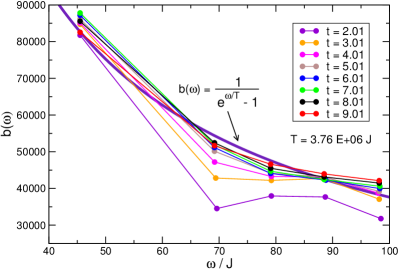
Figure 18: Distribution function $b(\tilde{\varepsilon}_{n},t)$ for different CoM times $t$. The thick purple line is a single-parameter fit of a thermal distribution to the calculated $b(\tilde{\varepsilon}_{n},t)$ for the largest time $t=9.01$, with temperatue $T$ as fit parameter. The fitted value is $T=3.76\cdot 10^{6}\ J$. Anna2016 Copyright 2016 by the American Physical Society.

To prove that the long-time state is a thermal one, we calculate the QP distribution function $b(\varepsilon_{n},t)$ for different CoM times $t$. It is defined via Keldysh Green’s functions Rammerbook by

$$F(\omega,t)=(-i/2)(2b(\omega,t)+1)A(\omega,t)$$ (89)

and is therefore obtained for each level from the Lorentzian weights $w_{A,n}$, $w_{F,n}$ of these levels (c.f. Fig. 17) as

$$b(\tilde{\varepsilon}_{n},t)=\frac{w_{F,n}}{w_{A,n}}-\frac{1}{2}\ .$$ (90)

Here $\tilde{\varepsilon}_{n}$, $n=1,\,\dots,\,M$, $(M=5)$, are the level energies, renormalized by interactions. As shown in Fig. 18, $b(\tilde{\varepsilon}_{n},t)$ continuously approaches a thermal distribution. As expected, the final-state temperature $T$ is high, since it is controlled by the initial BEC excitation energy, $\Delta E_{BEC}\sim z(0)^{2}N_{\textrm{tot}}J$, which is a macroscopically large quantity.

V Conclusions and Discussion

We demonstrated that the system of coupled, oscillating BECs and incoherent excitations thermalizes, because the condensates serve as a heat reservoir for the QP subsystem and visa versa. The QP subsystem is generated "naturally" as a result of complex non-equilibrium dynamics, in fact a parametric resonance. At a later time $\tau_{f}$ the energy of QP subsystem reaches its maximum value determined by the difference between the condensate initial and final energies, and the two subsystems become essentially decoupled in the grand canonical sense. The main reason for such a decoupling is total energy conservation and entropy maximization in the QP subsystem Anna2016 .

For times smaller than $\tau_{f}$, the condensate and the QPs are strongly coupled which is clearly seen in the resonating spectra of the two subsystems. For times $t>\tau_{f}$, BEC and incoherent excitations exhibit off-resonant behavior, confirming the decoupling. This is the essence of DBG.

In the off-resonant regime, the QP system relaxes slowly to a high-temperature thermal state with thermalization time $\tau_{th}>\tau_{f}$. The BEC freeze-out and subsequent time evolution under a conservation law are reminiscent of pre-thermalization found in low-dimensional, nearly integrable systems Joerg_review . However, our system is non-integrable, and the (approximate) conservation law is dynamically generated.

Remarkably, the non-equilibrium dynamics of the trapped Bose-gas system resembles the preheating and thermalization dynamics of inflationary models of the early universe Kofman1994 , see also Ref. Zache2017 . The Bose gas is initially prepared in a non-equilibrium state, analogous to the inflationary period of the early universe. The coherent Josephson oscillations of the BEC subsystem correspond to the the excitations of an inflaton field, postulated by the early-universe models Kofman1994 . The creation of QP excitation in the Bose gas system represents the creation of elementary particles after the inflationary period of the early universe. In both, the Bose gas system and the early universe, a parametric resonance emerges dynamically, between BEC Josephson oscillations and QP excitations on one hand, and between inflaton-field oscillations and elementary particles on the other hand. Finally, the effective decoupling of our bosonic subsystems corresponds to the inflaton decoupling due to loss of resonance by expansion of the universe. These analogies are worth further exploration Zache2017 .

Appendix A Notes on Numerical Implementation

In order to solve numerically our system of integro-differential equations, we discretize the two time arguments, $t$ and $t^{\prime}$ with a constant time-step $\Delta t$ (see Fig. 19). As a result, our spectral and statistical functions become matrices in the two-dimensional time plane. For instance,

$$\text{F}(t,t^{\prime})=\begin{pmatrix}\text{F}(0,0)&\text{F}(0,\Delta t)&\cdots&\text{F}(0,n\Delta t)\\ \text{F}(\Delta t,0)&\text{F}(\Delta t,\Delta t)&\cdots&\text{F}(\Delta t,n\Delta t)\\ \vdots&\vdots&\ddots&\vdots\\ \text{F}(n\Delta t,0)&\text{F}(n\Delta t,\Delta t)&\cdots&\text{F}(n\Delta t,n\Delta t)\end{pmatrix}$$

(91)

where both time arguments are counted from $\tau_{c}$, which is a finite time-scale at which the non-equilibrium dynamics sets in Mauro2015 , so that $\text{F}^{G}(0,0)\equiv\text{F}^{G}(\tau_{c},\tau_{c})$ etc. Both time scales go up to $t_{max}=n\Delta t$. In our case $t_{max}=10$. Fortunately, due to the symmetry relations (44) it is sufficient to calculate only half of the components of our propagators, i.e. the triangular matrix

$$\text{F}(t,t^{\prime})_{tri}=\begin{pmatrix}\text{F}(0,0)&\text{F}(0,\Delta t)&\cdots&\text{F}(0,n\Delta t)\\ 0&\text{F}(\Delta t,\Delta t)&\cdots&\text{F}(\Delta t,n\Delta t)\\ \vdots&\vdots&\ddots&\vdots\\ 0&0&\cdots&\text{F}(n\Delta t,n\Delta t),\end{pmatrix}$$

which is reflected in the time-plane grid in Fig.19. The blue points on the grid constitute additional copies of the diagonal (propagators with equal time arguments) contributions, necessary to properly perform the fourth order Runge-Kutta method. Symmetry relations for the self-energies (79) also contribute to simplifications, as we can rewrite all the integrands in Eqs. (80), (81) with time argument corresponding to later time on the left, e.g. time convolutions in the equation of motion for $F^{G}$ can be rewritten as

$$-i\int_{0}^{t}d{\overline{t}}\left[\Gamma^{G}_{n\ell}(t,{\overline{t}})\text{F}^{G}_{\ell m}({\overline{t},t^{\prime}})+\Gamma^{F}_{n\ell}(t,{\overline{t}})\text{F}^{\overline{F}}_{\ell m}({\overline{t}},t^{\prime})\right]$$

$$+i\int_{0}^{t}d{\overline{t}}\left[\Pi^{G}_{n\ell}(t,{\overline{t}})\text{A}^{G}_{\ell m}({\overline{t},t^{\prime}})+\Pi^{F}_{n\ell}(t,{\overline{t}})\text{A}^{\overline{F}}_{\ell m}({\overline{t}},t^{\prime})\right]$$

$$=i\int_{0}^{t^{\prime}}d{\overline{t}}\left[\Gamma^{G}_{n\ell}(t,{\overline{t}})\text{F}^{G}_{\ell m}(t^{\prime},{\overline{t}})^{*}+\Gamma^{F}_{n\ell}(t,{\overline{t}})\text{F}^{F}_{\ell m}(t^{\prime},{\overline{t}})^{*}\right]$$

$$-i\int_{t^{\prime}}^{t}d{\overline{t}}\left[\Gamma^{G}_{n\ell}(t,{\overline{t}})\text{F}^{G}_{\ell m}({\overline{t},t^{\prime}})-\Gamma^{F}_{n\ell}(t,{\overline{t}})\text{F}^{F}_{\ell m}({\overline{t}},t^{\prime})^{*}\right]$$

$$+i\int_{0}^{t^{\prime}}d{\overline{t}}\left[\Pi^{G}_{n\ell}(t,{\overline{t}})\text{A}^{G}_{\ell m}(t^{\prime},{\overline{t}})^{*}+\Pi^{F}_{n\ell}(t,{\overline{t}})\text{A}^{F}_{\ell m}(t^{\prime},{\overline{t}})^{*}\right]$$

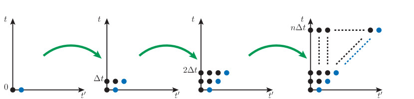
Figure 19: Evolution of the time grid in the two-time plane.

In non-equilibrium it is conventional to introduce mixed or Wigner coordinates: $\tau=t-t^{\prime}$ and $T=(t+t^{\prime})/2$ and then Fourier transform spectral functions and statistical functions with respect to the relative coordinate. In this way one can extract information about spectrum and distribution function for different values of $T$ and check if system approaches equilibrium with increasing $T$. In our case it is done by reading off the calculated spectral and statistical functions belonging to diagonals with the slope equal to $-1$ from the $t-t^{\prime}$ plane in Fig. 19. Those will be data for fixed $T$-s. We then Fourier transform them with respect to $\tau$. We checked the numerical accuracy by varying the time step $dt$ used in the differential equation solver. All the results are reproducible and independent of $dt$.

Appendix B Convolution Integrals in Equations of Motion

We use the symmetry relations (44), (74), (79) also in the convolution integrals which enter our equations of motion (80) and (81). Consider, for example, integrals in (81)

$$-\mathbbm{i}\sum_{k}\int\limits_{0}^{t}d\overline{t}[\Gamma^{G}_{ik}(t,\overline{t})\text{F}^{G}_{kj}(\overline{t},t^{\prime})+\Gamma^{F}_{ik}(t,\overline{t})\text{F}^{\overline{F}}_{kj}(\overline{t},t^{\prime})]$$ (94)

$$+\mathbbm{i}\sum_{k}\int\limits_{0}^{t^{\prime}}d\overline{t}[\Pi^{G}_{ik}(t,\overline{t})\text{A}^{G}_{kj}(\overline{t},t^{\prime})+\Pi^{F}_{ik}(t,\overline{t})\text{A}^{\overline{F}}_{kj}(\overline{t},t^{\prime})].$$

The symmetry relations allow us to split the interval of integration in such a way that we can rewrite the integrals with the arguments corresponding to the later time as first arguments. Hence we get for integral (94)

$$\mathbbm{i}\sum_{k}\int\limits_{0}^{t^{\prime}}d\overline{t}[\Gamma^{G}_{ik}(t,\overline{t})\text{F}^{G}_{jk}(t^{\prime},\overline{t})^{*}+\Gamma^{F}_{ik}(t,\overline{t})\text{F}^{F}_{jk}(t^{\prime},\overline{t})^{*}]$$ (95)

$$-\mathbbm{i}\sum_{k}\int\limits_{t^{\prime}}^{t}d\overline{t}[\Gamma^{G}_{ik}(t,\overline{t})\text{F}^{G}_{kj}(\overline{t},t^{\prime})-\Gamma^{F}_{ik}(t,\overline{t})\text{F}^{F}_{kj}(\overline{t},t^{\prime})^{*}]$$

$$+\mathbbm{i}\sum_{k}\int\limits_{0}^{t^{\prime}}d\overline{t}[\Pi^{G}_{ik}(t,\overline{t})\text{A}^{G}_{jk}(t^{\prime},\overline{t})^{*}+\Pi^{F}_{ik}(t,\overline{t})\text{A}^{F}_{jk}(t^{\prime},\overline{t})].$$

With the other integrals of Eqs. (80),(81), we proceed in analogous way and then solve the final system of equations numerically.

References

- (1) S. Trotzky, Y.-A. Chen, A. Flesch, I. P. McCulloch, U. Schollwöck, J. Eisert, I. Bloch, Nature Phys. 8, 325 (2012).
- (2) M. Gring, M. Kuhnert, T. Langen, T. Kitagawa, B. Rauer, M. Schreitl, I. Mazets, D. A. Smith, E. Demler, J. Schmiedmayer, Science 337, 1318 (2012).
- (3) A. Polkovnikov, K. Sengupta, A. Silva, M. Vengalattore, Rev. Mod. Phys. 83, 863 (2011).
- (4) V. I. Yukalov, Laser Phys. Lett. 8, 485 (2011).
- (5) J. M. Deutsch, Phys. Rev. A 43, 2046 (1991).
- (6) M. Srednicki, Phys. Rev. E 50, 888 (1994).
- (7) M. Rigol, V. Danjko, M. Olshanii, Nature 452, 854 (2008).
- (8) L. D’Alessio, Y. Kafri, A. Polkovnikov, M. Rigol, Advances in Physics 65, 239 (2016).
- (9) S. Goldstein, J. L. Lebowitz, R. Tumulka, N. Zanghi, Phys. Rev. Lett. 96, 050403 (2006).
- (10) P. Reimann, Phys. Rev. Lett. 115, 010403 (2015).
- (11) B. Pozsgay, J. of Stat. Mech.: Theory and Experiment, P09026 (2014).
- (12) V. Alba, Phys. Rev. B 91, 155123 (2015).
- (13) C. Kollath, A. Läuchli, E. Altmann, Phys. Rev. Lett. 98, 180601 (2007).
- (14) M. Moeckel, S. Kehrein, Phys. Rev. Lett. 100, 175702 (2008).
- (15) M. Kollar, F. A. Wolf, M. Eckstein, Phys. Rev. B 84, 054304 (2011).
- (16) T. Langen, T. Gansenzer, J. Schmiedmayer, Prethermalization and universal dynamics in near-integrable quantum systems, cond-mat arXiv:1603.09385 (2016).
- (17) M. Trujillo-Martinez, A. Posazhennikova, J. Kroha, Phys. Rev. Lett. 103, 105302 (2009).
- (18) M. Trujillo-Martinez, A. Posazhennikova, J. Kroha, New. J. Phys. 17, 013006 (2015).
- (19) A. Posazhennikova, M. Trujillo-Martinez, J. Kroha, Phys. Rev. Lett. 116, 225304 (2016).
- (20) L. D. Landau, E. M. Lifshits, Statistical Physics, Volume V, Elsevier (1980).
- (21) A. I. Khinchin, Mathematical foundations of statistical mechanics, Dover (1960).
- (22) Ya. G. Sinai, Introduction to Ergodic Theory, Princeton University Press (1977).
- (23) G. D. Birkhoff, Proc. Natl. Acad. Sci USA 17, 656 (1931).
- (24) J. von Neumann, Zeitschrift für Physik 57, 30 (1929).
- (25) N. Singh, Mod. Phys. Lett. B 27, 1330003 (2013).
- (26) M. Rigol, M. Srednicki, Phys. Rev. Lett. 108, 110601 (2012).
- (27) H. Aoki, N. Tsuji, M. Eckstein, M. Kollar, T. Oka, P. Werner, Rev. Mod. Phys. 86, 779 (2014).
- (28) H. U. R. Strand, M. Eckstein, P. Werner, Phys. Rev. X 5, 011038 (2015).
- (29) U. Schollwöck, Rev. Mod. Phys. 77, 259 (2005).
- (30) G. Roux, Phys. Rev. A 79, 021608(R) (2009).
- (31) B. D. Josephson, Phys. Lett. 1, 251 (1962).
- (32) J. Javanainen, Phys. Rev. Lett. 57, 3164 (1986).
- (33) A. Smerzi, S. Fantoni, S. Giovanazzi, S. R. Shenoy, Phys. Rev. Lett. 79, 4950 (1997).
- (34) M. Albiez, R. Gati, J. Fölling, S. Hunsmann, M. Cristiani, M. K. Oberthaler, Phys. Rev. Lett. 95, 010402 (2005).
- (35) S. Levy, E. Lahoud, I. Shomroni, J. Steinheuer, Nature 449, 579 (2007).
- (36) L. J. LeBlanc, A. B. Bardon, J. McKeever, M. H. T. Extavour, D. Jervis, J. H. Thywissen, F. Piazza, A. Smerzi, Phys. Rev. Lett. 106, 025302 (2011).
- (37) G. Milburn, J. Corney, E. Wright, D. Walls, Phys. Rev. A 55, 4318 (1997)
- (38) R. Gati, M. K. Oberthaler, J. Phys. B: At. Mol. Opt. Phys. 40, R61 (2007).
- (39) I. Zapata, F. Sols, A. J. Leggett, Phys. Rev. A 57, R28 (1998).
- (40) I. Zapata, F. Sols, A. J. Leggett, Phys. Rev. A 67, 021603(R) (2003).
- (41) L. Pitaevskii, S. Stringari, Phys. Rev. Lett. 87, 180402 (2001).
- (42) J. Esteve et al., Nature (London) 455, 1216 (2008).
- (43) A. Smerzi, A. Trombettoni, Phys. Rev. A 68, 023613 (2003).
- (44) R. Gati, Bose-Einstein Condensates in a Single Double Well Potential, Dissertation, 2007.
- (45) D. Ananikian, T. Bergeman, Phys. Rev. A 73, 013604 (2006).
- (46) J. Berges, "Introduction to Nonequilibrium Quantum Field Theory", AIP Conf. Proc. 739, 3 (2004).
- (47) A. M. Rey, B. L. Hu, E. Calzetta, C. W. Clark, Phys. Rev. A 72, 023604 (2005).
- (48) J. Rammer, Quantum Field Theory of Non-equilibrium States, Cambridge University Press (2007).
- (49) L. P. Kadanoff, G. Baym, Quantum Statistical Mechanics, New York: Banjamin (1968).
- (50) A. Griffin, T. Nikuni, E. Zaremba, Bose-Condensed Gases at Finite Temperatures, Cambridge University Press (2009).
- (51) M. Trujillo-Martinez, A. Posazhennikova, J. Kroha, in preparation.
- (52) T. Lappe, A. Posazhennikova, J. Kroha, in preparation.
- (53) V. I. Yukalov, E. P. Yukalova, Phys. Rev. A 78, 063610 (2008).
- (54) L. Kofman, A. Linde, A. A. Starobinsky, Phys. Rev. Lett. 73, 3195 (1994).
- (55) T. V. Zache, V. Kasper, J. Berges, arXiv:1704.02271 (2017).