Polytypism in the ground state structure of the Lennard-Jonesium

Abstract

We present a systematic study of the stability of nineteen different periodic structures using the finite range Lennard-Jones potential model discussing the effects of pressure, potential truncation, cutoff distance and Lennard-Jones exponents. The structures considered are the hexagonal close packed (hcp), face centred cubic (fcc) and seventeen other polytype stacking sequences, such as dhcp and $9R$. We found that at certain pressure and cutoff distance values, neither fcc nor hcp is the ground state structure as previously documented, but different polytypic sequences. This behaviour shows a strong dependence on the way the tail of the potential is truncated.

I Introduction

Polytypism is a special form of polymorphism, occurring in layered materials, in which the polymorphs are derived simply by varying the way in which the layers are arranged relative to each other. This means that the various stacking arrangements do not affect the chemistry of the phase as a whole, but some of the physical properties (e.g. density, Young modulus, band gap or electron mobility) can be significantly different. A large variety of materials have several different stable polytype phases Trigunayat (1991), one of the most extensively studied being SiC Jepps and Page (1983); Nakashima and Hangyo (1991). SiC has more than 200 identified polytypes, a few being more favoured in applications than the rest due to their superior electronic properties. Many materials with similar structural properties also form polytypes, such as metal sulphides and halogenides, e.g. ZnS Mardix et al. (1969); Boutaiba et al. (2014) and CdI₂ Katahama et al. (1984). The physical properties of such materials can be tuned by changing the stacking sequences, e.g. in ZnO Zagorac et al. (2015). Polytypism also occurs in the case of diamond. The common cubic form of diamond has a hexagonal polytype called Lonsdaleite, which is suggested to be a complex mixture of different stacking sequences Wen et al. (2008); Salzmann et al. (2015). Similarly, hexagonal (Ih) and cubic (Ic) ice are also polytypic structures. Some elements are also known to form polytype phases, such as lanthanum, which exists in the dhcp form Bağci et al. (2010), samarium and lithium having the $9R$ stacking sequence as the ground state structure Ellinger and Zachariasen (1953); Overhauser (1984), erbium which is stable in both dhcp and 9R stacking sequences at different pressures Samudrala et al. (2011), and bismuth, long suspected to exist in several polytypic forms Shu et al. (2016). It has been speculated that the transformation from fcc to hcp structure with increasing pressure might occur through a series of different stacking fault structures, e.g. as in the case of noble gases xenon and krypton, suggested by some experimental results Jephcoat et al. (1987); Errandonea et al. (2002), or in the case of iron at high pressure and high temperature Yoo et al. (1996); Mikhaylushkin et al. (2007). Finally, if a wider definition of polytypism is used such that structurally compatible modules are also considered, a range of minerals which include the pyroxenes, perovskites, spinelloids, chlorites and oxides form polytypic structures as well Price and Yeomans (1984).

In order to model the polytypic behaviour, the axial next-nearest-neighbour Ising (ANNNI) model, was used in the 1980s Price and Yeomans (1984); J Yeomans and G D Price (1986); J Yeomans (1988). (An overview of the ANNNI and A3NNI ground state structures are given in the Appendix.) However, the two possible layer types in ANNNI, usually marked by $\downarrow$ and $\uparrow$ are interchangeable, a phase is only defined by the number of consecutive layers of the same orientation, but not the orientation of the layer itself, thus phases $\downarrow\downarrow\uparrow$ and $\uparrow\uparrow\downarrow$ are identical. In contrast, close packed stacking structures are built up by layers in three different possible positions, usually denoted by A, B and C, forming either a hexagonal (in ABA stacking) or a cubic (in ABC stacking) layer. These two are not identical nor interchangeable, meaning that the ability of ANNNI to describe the behaviour of close packed materials is limited.

One of the most widely used models to study close-packed materials is the Lennard-Jones pair potential. It has been long known that its low temperature dominant structures are the hexagonal close packed (hcp) and the face centred cubic (fcc) Kihara and Koba (1952). Interestingly, although other structures (bcc, simple cubic, diamond) have been studied Travesset (2014), to the best of our knowledge no other polytype sequences have ever been investigated from the point of view of phase stability, only as stacking faults in relation to crystal growth defects or nucleation de Souza and Wales (2016). It is also notable that the customary finite range truncation of the potential has a significant effect on the liquid-vapour equilibrium Smit (1992); Panagiotopoulos (1994); Shi and Johnson (2001) and on the melting temperature Mastny and de Pablo (2007); Ahmed and Sadusa (2010), yet it is rarely mentioned and almost never taken into account in the discussion of the low temperature solid phases, causing an apparent inconsistency in the literature with regard to the lowest energy structure: some works refer to the fcc de Souza and Wales (2016); van der Hoef (2000), others to hcp van de Waal (1991); Travesset (2014) as the global minimum of the Lennard-Jones model. An exception is an article by Jackson et. al Jackson et al. (2002) showing that the ground state can be either fcc or hcp depending on the cutoff distance and method of truncation.

Our aim in this work is to provide a systematic study of the ground state structure of the Lennard-Jones potential considering different polytypic stacking sequences, and fill the gap in the literature regarding its dependence on pressure, potential truncation and potential parameters. The rich diversity of structures we find serve as a reminder that complex material behaviour can result from comparatively simple models, and that implementation details can have a strong effect on phase stability when modelling materials.

II Computational details

A generalised form of the Lennard-Jones potential can be given by

$$U_{\mathrm{LJ}}(r)=\frac{p}{(p-q)(\frac{q}{p})^{q/(p-q)}}\epsilon\bigg{[}\Big{(}\frac{\sigma}{r}\Big{)}^{p}-\Big{(}\frac{\sigma}{r}\Big{)}^{q}\bigg{]}.$$ (1)

The values $p=12$ and $q=6$ are most common, in which case one obtains

$$U_{\mathrm{LJ}}(r)=4\epsilon\bigg{[}\Big{(}\frac{\sigma}{r}\Big{)}^{12}-\Big{(}\frac{\sigma}{r}\Big{)}^{6}\bigg{]},$$ (2)

where $\epsilon$ is the depth of the potential well, $\sigma$ is the size of the repulsive core and $r$ is the distance between two particles. This potential is usually truncated at a cut-off distance, $r_{c}$, and to avoid the discontinuity at this point, the potential can be shifted. The energy-shifted LJ potential is a continuous ($C^{0}$) function,

$$U_{\mathrm{LJ}-C^{0}}(r)=\begin{cases}U_{\mathrm{LJ}}(r)-U_{\mathrm{LJ}}(r_{c})&r\leq r_{c}\\ 0&r>r_{c}.\\ \end{cases}$$ (3)

In order to obtain continuous forces at the cut-off distance, and thus make the potential function differentiable, it can be force-shifted, which leads to

$$U_{\mathrm{LJ}-C^{1}}(r)=\begin{cases}\!\begin{aligned} U_{\mathrm{LJ}}(r)&-U_{\mathrm{LJ}}(r_{c})-\\ &-(r-r_{c})U^{\prime}_{\mathrm{LJ}}(r_{c})\end{aligned}&r\leq r_{c}\\ 0&r>r_{c}.\\ \end{cases}$$ (4)

In order to make also the second derivatives continuous at $r_{c}$ (i.e. create a $C^{2}$ function), the potential can be further shifted by a third term,

$$U_{\mathrm{LJ}-C^{2}}(r)=\begin{cases}\!\begin{aligned} U_{\mathrm{LJ}}(r)-U_{\mathrm{LJ}}(r_{c})&\\ -(r-r_{c})U^{\prime}_{\mathrm{LJ}}(r_{c})&\\ -{\textstyle\frac{1}{2}}(r-r_{c})^{2}U^{\prime\prime}_{\mathrm{LJ}}(r_{c})&\end{aligned}&r\leq r_{c}\\ 0&r>r_{c}.\\ \end{cases}$$ (5)

Alternatively, a sigmoidal shaped function, $f_{s}(r)$, can be used to ”smooth out” the force shifted potential within a distance $r_{s}$ of the cutoff,

$$U_{\mathrm{LJ}-C^{1}-\mathrm{smoothed}}(r)=f_{s}(r)U_{\mathrm{LJ}-C^{1}}(r).$$ (6)

For $f_{s}(r)$ we used an infinitely differentiable ($C^{\infty}$) function,

$$f_{s}(r)\begin{cases}1&r\leq(r_{c}-r_{s})\\ 1-\frac{e^{(-1/x)}}{e^{(-1/x)}+e^{(-1/(1-x))}}&(r_{c}-r_{s})<r\leq r_{c}\\ 0&r>r_{c},\\ \end{cases}$$ (7)

where $x=[r-(r_{c}-r_{s})]/r_{s}$).

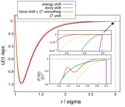
Figure 1: Shape of the Lennard-Jones potential of exponents $p=12$ and $q=6$, with different cutoff schemes. All functions were used with cutoff distance $r_{c}=3.0\sigma$ and in case of the smoothed force-shifted potential, $r_{s}=1.0\sigma$ smoothing range has been used. The top inset shows the functions at the vicinity of the cutoff, while the bottom inset shows the second derivative at the potentials.

Table 1: Different stacking variants studied, listed with both their hc and ABC notation. Alternative names and Ramsdell notations are shown for specific stacking sequences in parenthesis.

stacking	min. number	physical stacking of the layers
variants	of layers
c (fcc, $3C$)	3	$[ABC]_{n}$
h (hcp, $2H$)	2	$[AB]_{n}$
hc (dhcp,$4H$)	4	$[ABCB]_{n}$
hcc (thcp,$6H_{1}$)	6	$[ABCACB]_{n}$
hccc	8	$[ABCABACB]_{n}$
hcccc	10	$[ABCABCBACB]_{n}$
hccccc	12	$[ABCABCACBACB]_{n}$
hhc ($9R$)	9	$[ABACACBCB]_{n}$
hhcc	12	$[ABACBCBACACB]_{n}$
hhccc	5	$[ABACB]_{n}$
hhcccc	18	$[ABACBACACBACBCBACB]_{n}$
hhhc	8	$[ABABCBCB]_{n}$
hhhcc	10	$[ABABCACACB]_{n}$
hhhccc	12	$[ABABCABABACB]_{n}$
hhhhc	15	$[ABABACACACBCBCB]_{n}$
hhhhcc	18	$[ABABACBCBCBACACACB]_{n}$
hhhhhc	12	$[ABABABCBCBCB]_{n}$
hchcc ($15R$)	15	$[ABCBACABACBCACB]_{n}$
hchhc	10	$[ABCBCACBCB]_{n}$

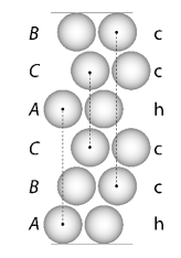
Figure 2: An example snapshotLi (2003) of the $\langle\mathrm{hcc}\rangle$ sequence. Layers at the same lateral position are connected by dashed lines.

Nineteen different stacking sequences were considered (shown in Table 1), all variations up to five stacking layers, and some of the possible six layer arrangements. The notation used to mark the sequences is that layers with fcc surroundings (the two neighbouring layers occupy different positions) is marked “c” as cubic, while the layers with hcp surrounding (sandwiched between two layers occupying the same position) is marked “h” as hexagonal. An example structure, with associated notation, is shown in Figure 2.

The geometry optimisations were performed with the QUIP package qui , with the conjugate gradient method and double-checked with the steepest descent method for several cases. The minimisation tolerance was set to $10^{-6}\epsilon/\sigma$ for the norm of the forces, which corresponds to $10^{-15}\epsilon/\mathrm{atom}$ accuracy in the energy calculation. Hydrostatic pressure was applied. The minimisations were started from configurations where atoms were placed $1.0\sigma$ distance from each other, and during the minimisation the atomic positions and all the lattice parameters were allowed to relax. The calculations were done with different shifted and smoothed versions of the potential to compare their effects within the truncation range $2.0\sigma\leq r_{c}\leq 6.0\sigma$, in $0.05\sigma$ intervals.

III Results: ground state phase diagrams of the Lennard-Jones potential

During the minimisation process configurations retained their stacking order, and the atoms forming the stacking plane also stayed perfectly in the plane. Lattices remained orthorhombic, but the lattice height corresponding to the stacking direction changed with respect to the other two, as expected. To be able to identify the ground state structures and draw the phase diagrams, the enthalpies of the minimised configurations were calculated and compared. These enthalpy curves were individually checked and more calculations were performed with a finer pressure scale whenever it was necessary, thus we believe that no phases have been missed. A set of example enthalpy curves can be seen on Figure 3.

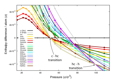
Figure 3: Enthalpy difference of different polytypes relative to that of the fcc structure as a function of pressure. The potential is force shifted and cutoff is $r_{cut}=2.7\sigma$. The arrows show the location of the two phase transitions where the enthalpy of several polytypes are almost equal due to the relatively short cutoff, thus the phase boundary between $\langle\mathrm{c}\rangle$ and $\langle\mathrm{hc}\rangle$ is close to being a multiphase boundary with $\langle\mathrm{hc}^{k}\rangle$ and $\langle\mathrm{hchcc}\rangle$ type polytypes, while the boundary between $\langle\mathrm{h}\rangle$ and $\langle\mathrm{hc}\rangle$ is degenerate with $\langle\mathrm{h}^{k}\mathrm{c}\rangle$ and $\langle\mathrm{hchhc}\rangle$ type sequences. This behaviour becomes less prominent as the cutoff increases.

Truncation distance vs. pressure phase diagrams of the Lennard-Jones type potentials with different cutoff schemes are shown on Figures 4, 5 and 6. The coloured regions show the series of phases found to be the most stable at a given truncation length and in a given pressure range. Dark grey colour corresponds to the fcc and light grey to hcp structures, with other colours representing different stacking variants (yellow and red shades represent stackings with a single “h” layer in the repeated subunit, green shades are polytypes with two consecutive “h” layers, while blues and purples correspond to three and four consecutive “h” layers, respectively).

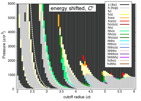
Figure 4: Lennard-Jones ground state structures as a function of cut-off radius and pressure. The potential is $C^{0}$, i.e. energy shifted. The colours represent the different stacking sequences, dark grey is pure fcc and light grey is pure hcp. The white dashed line demonstrates one of the boundaries along which a new shell of atoms gets inside the cutoff sphere.

It is clear from all the phase diagrams, that the hcp structure tends to be the most favourable stacking variant at lower pressure values, while for every value of the cutoff there is a pressure above which the fcc is the most stable polytype. In order to see whether one of the studied polytypes becomes the ground state again at even higher pressures, the structures were minimised up to $p=6\times 10^{5}\epsilon/\sigma^{3}$ for a few randomly chosen cutoffs: fcc remained the lowest enthalpy structure in every case.

However, the most striking result is that at the boundary between the ground state regions of fcc and hcp structures, several other stacking variants are found to be more stable. This means that, in contrast with the common belief, the (truncated) Lennard-Jones potential exhibits a wide range of different global minima depending on the fine details of the potential.

The boundary between the fcc and hcp regions appear to have a “wave”-like pattern for all the potential function variants we used. The shape of these waves reflect how the distance of atomic shells decreases as the density increases with increasing pressure. (The white dashed graph in Figure 4 represents the curve along which the number of atoms within the cutoff radius jumps from 177 to 201 in the fcc crystal.) As different polytypes have different numbers of neighbours in each shell, their relative energy will be different depending on which shells lie within the cutoff radius. As the pressure increases the atoms get closer, farther shells appear within the smaller cutoff radii, causing the phase boundary to be shifted towards smaller cutoffs.

At small cutoff values, fewer polytypes appear along the fcc-hcp boundary and these remain the same as the pressure increases. As the number of shells are increased using larger cutoffs, this is no longer true, due to the fact that the distance between the layers of fcc and hcp can be different depending on the pressure, thus the neighbour shells will no longer be isotropic. Finally, with increasing cutoff, the energy contribution of the outmost shells gets smaller, the “waves” gradually flatten out.

Figure 4 shows the phase diagram of the simple energy shifted Lennard-Jones function (see eq. 3). At smaller cutoff values, only one phase is found to be stable other than fcc and hcp, the $\langle\mathrm{hc}\rangle$ phase. As the cutoff increases, first the $\langle\mathrm{hhc}\rangle$ and $\langle\mathrm{hhcc}\rangle$ phases appear, than other sequences with longer repeated subunits as well.

Applying additional shifts to the potential, such as force-shift and second-derivative shift, the “wave” like pattern of the phase diagram becomes significantly less pronounced (see the first two panels of Figure 5), but the order in which the more complex polytypes appear on the phase diagram remains similar. For example $\langle\mathrm{hhc}\rangle$ and $\langle\mathrm{hhcc}\rangle$ phases appear on the second “wave”, the same two and $\langle\mathrm{hc}\rangle$ on the two sides of the third “wave” and then $\langle\mathrm{hcccc}\rangle$ first appears on the tip of the fourth “wave” in all three phase diagrams. Although we are unable to offer a rigorous explanation for the flattening trend of the “waves”, we speculate that it is due to the fact that a non-smooth cut-off mechanism leads to large variations in energy as new neighbour shells cross the interaction range. Since different polytypes have different neighbour shells, significant changes in energy differences can therefore occur.

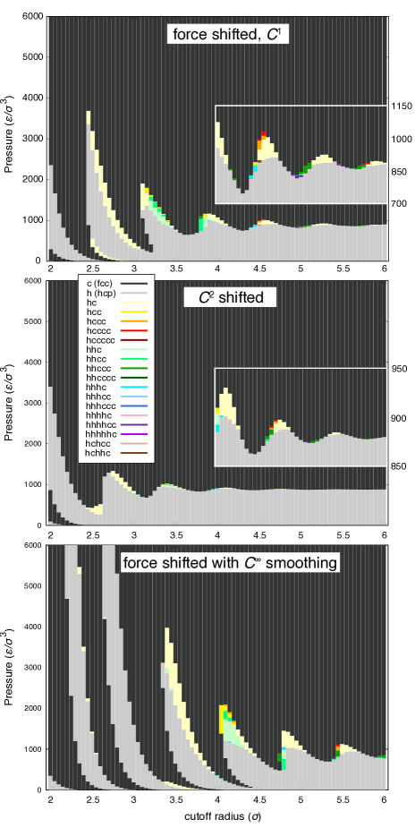
Figure 5: Lennard-Jones ground state structures as a function of cut-off radius and pressure. In the top panel the potential is force shifted, the middle panel shows the $C^{2}$ shifted potential (see eq. 5), while the bottom panel shows the force shifted potential with a $C^{\infty}$ smoothing function (see e.q. 7) applied in the $1.0\sigma$ range of the cutoff. The colours represent the different stacking sequences. The insets show the phase boundaries between cutoffs $4.0\sigma$ and $6.0\sigma$ enlarged, the different pressure scale shown on the right.

Using a smoothing function to obtain a completely smooth potential, $U_{{\rm LJ}-C^{\infty}}$ has seemingly the opposite effect, while the width of the stability region of the $\langle\mathrm{hc}\rangle$ phase becomes significantly narrower, especially at shorter cutoffs, the magnitude of the “waves” increases (see Figure 5). The explanation for this effect is that $U_{\rm LJ-C^{\infty}}$ is only qualitatively smooth but not quantitively. Indeed we observe in Figure 1 that its second derivative has rapid variations in the interval where the cut-off is applied. It also has to be noted that the exact effect of the smoothing will also depend on the widths of the smoothing region.

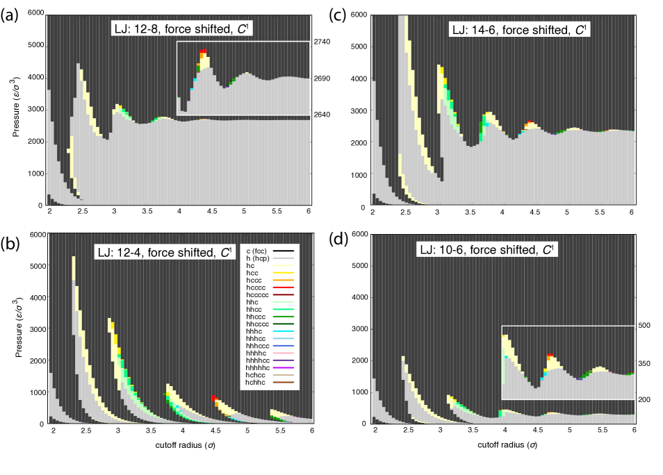
Figure 6: Ground state structure of Lennard-Jones potential with different exponents (a) $p=12$ and $q=8$, (b) $p=12$ and $q=4$, (c) $p=14$ and $q=6$, (d) $p=10$ and $q=6$ as a function of cut-off radius (in sigma units) and pressure. The potential is force shifted. The colours represent the different stacking sequences, dark grey is pure fcc and light grey is pure hcp. The insets show the phase boundaries between cutoffs $4.0\sigma$ and $6.0\sigma$ enlarged, the different pressure scale shown on the right.

In order to study the effect of the Lennard-Jones exponents, thus the shape of the pair potential on the ground state phase diagram, we repeated our calculations on the force shifted potential with the following different $p$ and $q$ exponents: 12 and 8, 12 and 4, 14 and 6, 10 and 6. The phase diagrams are shown in Figure 6. It is clear from these figures that changing the exponents does not notably change the order in which the polytypic phases appear to be stable, thus the same stacking variants appear at the same cutoff values, but the corresponding pressure of the phase transitions are significantly different. As a general rule, if either of the exponents are increased, the pressure above which the fcc phase is the most stable increases as well.

IV Other interatomic potentials

IV.1 Power law potential

A simple repulsive power law potential with the exponent set to 12,

$$U_{\mathrm{pl}}(r)=4\epsilon\Big{(}\frac{\sigma}{r}\Big{)}^{12},$$ (8)

was also tested to see whether polytypic phases are stable in this case. A force-shift was applied here as well. The results indicate that the ground state structure is fcc at every pressure and cutoff studied.

IV.2 Morse potential

In order to see how another simple pair potential with an attractive term behave we also tested the Morse potential,

$$U_{\mathrm{M}}(r)=D_{e}\Big{(}e^{-2a(r-r_{e})}-2e^{-a(r-r_{e})}\Big{)},$$ (9)

with parameters $D_{e}=1.0$, $r_{e}=1.0$ controlling the depth and location of the minimum, respectively, and $a=4.0$. (We chose the value for parameter $a$ so that the pair potential is similar in shape to the Lennard-Jones potential.) The potential was force shifted. The Morse phase diagram (see Figure 7) shows some stacking fault structures too: $\langle\mathrm{hc}\rangle$, $\langle\mathrm{hhc}\rangle$ and $\langle\mathrm{hhcc}\rangle$, similarly to the LJ potential, but only at small cutoffs. Above $r_{cut}=3.6r_{e}$ the fcc is the only stable phase. This fast decay of the “waves” can be explained by the exponential decay of the potential function, but the fact that polytypes other than fcc and hcp are found to be ground states also in case of the Morse potential indicates that the results we obtained for Lennard-Jones potentials in the previous sections might be generic for truncated pair potentials.

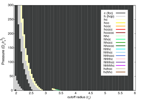
Figure 7: Morse potential ground state structures as a function of cut-off radius (in $r_{e}$ units) and pressure. The potential is force shifted. The colours represent the different stacking sequences, dark grey is pure fcc and light grey is pure hcp. (Note: the pressure axis is different to that of the LJ one to show the low pressure region in more details.)

V Conclusion

We have systematically studied the global minimum structure of the bulk Lennard-Jones model as a function of pressure and the details of potential truncation. Our results demonstrate that its ground state structures are far more complex than previously reported, the stable phases including not only fcc and hcp but a wide range of more complex stacking sequences. Most notably we obtained $\langle\mathrm{hc}\rangle$ and $\langle\mathrm{hhc}\rangle$ phases, the two polytypes most often observed in real materials (as dhcp and 9R) other then hcp and fcc. This suggests that well-known pair potentials might be useful models of polytypism and can help us to understand and predict polytypic behaviour.

The relative stability of polytypes was found to be especially sensitive to the degree of smoothness of the potential around the cutoff. This shows that the effect of truncation and the way the derivative of the potential is treated should not be underestimated when using pair potentials. Further work is still needed, however, to obtain a clear theoretical explanation for the polytypism that we observed, e.g. to construct potentials with prescribed polytypes, as well as to confirm analogous effects in case of more complex model systems.

Appendix A Stable structures of the ANNNI and A3NNI models

One of the simplest nontrivial models exhibiting periodically ordered phases, is the axial next-nearest-neighbour Ising model, ANNNI Elliott (1961); Fisher and Selke (1980), which is a variant of the Ising model with a two-state spin on each lattice site. Interactions are between nearest neighbours, together with a second-neighbour interaction along one lattice direction (this is the axial direction, $z$). The model is defined by the Hamiltonian

$$H=-\frac{1}{2}J_{0}\sum_{ijj^{\prime}}{S_{i,j}S_{i,j^{\prime}}}-J_{1}\sum_{ij}{S_{i,j}S_{i+1,j}}-J_{2}\sum_{ij}{S_{i,j}S_{i+2,j}}$$ (10)

where $S_{ij}$ is the two-state spin on each lattice site, and $i$ denotes the layers perpendicular to the axial direction and $j$ and $j^{\prime}$ are nearest neighbour spins within the layer.

The ANNNI model is considered a prototype for polytypism Price and Yeomans (1984); J Yeomans and G D Price (1986), since its phase diagram contains sequences of long-wavelength-modulated phases, hence showing that short-range competing interactions are sufficient to stabilise long periodic structures as ground states.

Within ANNNI, the layers building up the polytypes can be characterised by two signs, $\downarrow$ and $\uparrow$. In these models $\cdots\uparrow\uparrow\uparrow\cdots$ and $\cdots\downarrow\downarrow\downarrow\cdots$ are identical, and often simply marked as $\langle\infty\rangle$ (this is called the Zhdanov notation where the numbers in the brackets show the band widths, i.e. the number of layers with the same spin, e.g. $\langle 2\rangle$=(2,2) means $\cdots\uparrow\uparrow\downarrow\downarrow\cdots$).

The ground state phase diagram of ANNNI can be easily determined  Price and Yeomans (1984), see Figure 8. There are three main stable phases at 0 K, $\langle 1\rangle$, $\langle 2\rangle$ and $\langle\infty\rangle$, but the two dashed lines mark regions where the ground state is highly degenerate: along the line between $\langle 1\rangle$ and $\langle 2\rangle$ all phases containing only 1 and 2 bands have equal energy (e.g. $\langle 12\rangle$, $\langle 12^{2}\rangle$,…etc.), and along the line between $\langle 2\rangle$ and $\langle\infty\rangle$ all phases which contain no 1-bands have the same energy (e.g. $\langle 23\rangle$, $\langle 2^{2}4\rangle$, etc.). Note, that the boundary between $\langle 1\rangle$ and $\langle\infty\rangle$ is not degenerate! This means in particular that there are several phases missing from this phase diagram, e.g. $\langle 13\rangle$, $\langle 14\rangle$, and so forth, are not ground states at any value of $J_{1}$ or $J_{2}$.

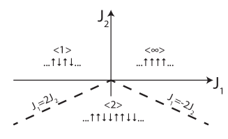
Figure 8: Ground states of the ANNNI model. Dashed lines mark multiphase boundaries.

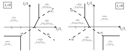
Figure 9: Ground states of the A3NNI model, in case $J_{1}<0$ (left hand side) and $J_{1}>0$ (right hand side). Dashed lines mark multiphase boundaries and correspond to the following structure groups; $(A)$: $\langle 2(12)^{k}\rangle$ and $\langle 2(12)^{k}2(12)^{k+1}\rangle$ for $J_{2}/J_{1}<0$ and for $J_{2}/J_{1}>0$ also $\langle(12)^{k}112(12)^{k-1}\rangle$, $(B)$: $\langle 2(12)^{k}\rangle$ and $\langle 2(12)^{k}2(12)^{k+1}\rangle$, $(D)$: phases containing 1 and 2 bands, $(E)$: $\langle 23^{k}\rangle$ and $\langle 23^{k}23^{k+1}\rangle$, $(F)$: $\langle 3^{k}4\rangle$ and for $J_{2}>0\langle 3^{k}43^{k+1}4\rangle$

In order to see how longer range interactions effect the stability of phases, the third neighbour Ising model, A3NNI has been studied too and discussed as a model for polytypism J Yeomans (1988); Muraoka et al. (1998); Salje et al. (1987). If the third neighbour interactions are also taken into account, the ground state phase diagram becomes more complicated and two additional structures appear as possible ground states phases compared to ANNNI, the $\langle 12\rangle$ and $\langle 3\rangle$ with several additional phases along the multiphase lines J Yeomans (1988); Salje et al. (1987); see Figure 9.

Many of the polytypic structures found in different materials resemble the phases seen in the ANNNI and A3NNI models. For example, PbI₂ has a reversible phase transition between the phases $\langle\infty\rangle$ and $\langle 1\rangle$, with the phases $\langle 2\rangle$ and $\langle 12\rangle$ being observed under different growth conditions only Salje et al. (1987). Same is true for ZnS and AgI. Phase transitions between $\langle 1\rangle-\langle 2\rangle-\langle\infty\rangle$ are found in MgSiO₃, and $\langle 1\rangle-\langle\infty\rangle-\langle 3\rangle-\langle 23\rangle$ are seen in case of SiC Jepps and Page (1983). However, there are also polytypic structures seen in experiments, e.g. $\langle 13\rangle$ in spinelloids, which do not occur in the ANNNI model.

At temperatures slightly above 0 K, the phase diagram remains similar but at the vicinity of the multiphase lines sequences of $\langle 12^{k}\rangle$ and $\langle 2^{k}3\rangle$ appear, and even more new phases at higher temperatures (though the proportion of disordered layers increase too) Fisher and Selke (1980).

References

- Trigunayat (1991) G. C. Trigunayat, Solid State Ionics 48, 3 (1991).
- Jepps and Page (1983) N. W. Jepps and T. F. Page, J. Cryst. Growth Charact. 7, 259 (1983).
- Nakashima and Hangyo (1991) S. Nakashima and M. Hangyo, Solid State Comm. 80, 21 (1991).
- Mardix et al. (1969) S. Mardix, I. Kiflawi, and Z. H. Kalman, Acta Crystallogr. B B25, 1586 (1969).
- Boutaiba et al. (2014) F. Boutaiba, A. Belabbes, M. Ferhat, and F. Bechstedt, Phys. Rev. B 89, 245308 (2014).
- Katahama et al. (1984) H. Katahama, S. Nakashima, M. Hangyo, A. Mitsuishi, and B. Palosz, Solid State Commun. 49, 547 (1984).
- Zagorac et al. (2015) D. Zagorac, J. C. Schön, J. Zagoracab, and M. Jansena, RSC Advances 5, 25929 (2015).
- Wen et al. (2008) B. Wen, J. Zhao, M. J. Bucknum, P. Yao, and T. Li, Diam. Relat. Mater. 17, 356 (2008).
- Salzmann et al. (2015) C. G. Salzmann, B. J. Murray, and J. J. Shephard, Diam. Relat. Mater. 59, 69 (2015).
- Bağci et al. (2010) S. Bağci, H. M. Tütüncü, S. Duman, and G. P. Srivastava, Phys. Rev. B. 81, 144507 (2010).
- Ellinger and Zachariasen (1953) F. H. Ellinger and W. H. Zachariasen, J. Am. Chem. Soc. 75, 5650 (1953).
- Overhauser (1984) A. W. Overhauser, Phys. Rev. Lett. 53, 64 (1984).
- Samudrala et al. (2011) G. K. Samudrala, S. A. Thomas, J. M. Montgomery, and Y. K. Vohra, J. Phys. Condens. Matter 23, 315701 (2011).
- Shu et al. (2016) Y. Shu, W. Hu, Z. Liu, G. Shen, B. Xu, Z. Zhao, J. He, Y. Wang, Y. Tian, and D. Yu, Sci. Rep. 6, 20337 (2016).
- Jephcoat et al. (1987) A. P. Jephcoat, H. K. Mao, L. W. Finger, D. Cox, R. J. Hemley, and C. S. Zha, Phys. Rev. Lett. 59, 2670 (1987).
- Errandonea et al. (2002) D. Errandonea, B. Schwager, R. Boehler, and M. Ross, Phys. Rev. B 65, 214110 (2002).
- Yoo et al. (1996) C. Yoo, P. Söderlind, J. Moriarty, and A. Cambell, Phys. Lett. A 214, 65 (1996).
- Mikhaylushkin et al. (2007) A. S. Mikhaylushkin, S. I. Simak, L. Dubrovinsky, N. Dubrovinskaia, B. Johansson, and I. A. Abrikosov, Phys. Rev. Lett. 99, 165505 (2007).
- Price and Yeomans (1984) G. D. Price and J. Yeomans, Acta Crystallogr. B 40, 448 (1984).
- J Yeomans and G D Price (1986) J Yeomans and G D Price, B. Minéral. 109, 3 (1986).
- J Yeomans (1988) J Yeomans, Solid State Phys. 41, 151 (1988).
- Kihara and Koba (1952) T. Kihara and S. Koba, J. Phys. Soc. Jpn. 7, 348 (1952).
- Travesset (2014) A. Travesset, The Journal of Chemical Physics 141 (2014).
- de Souza and Wales (2016) V. K. de Souza and D. J. Wales, Journal of Statistical Mechanics: Theory and Experiment 7, 074001 (2016).
- Smit (1992) B. Smit, J. Chem. Phys 96, 8639 (1992).
- Panagiotopoulos (1994) A. Z. Panagiotopoulos, Int. J. Thermophys. 15, 1057 (1994).
- Shi and Johnson (2001) W. Shi and J. K. Johnson, Fluid Phase Equilibr. 187–188, 171 (2001).
- Mastny and de Pablo (2007) E. A. Mastny and J. J. de Pablo, J. Chem. Phys 127, 104504 (2007).
- Ahmed and Sadusa (2010) A. Ahmed and R. J. Sadusa, J. Chem. Phys 133, 124515 (2010).
- van der Hoef (2000) M. A. van der Hoef, J. Chem. Phys. 113, 8142 (2000).
- van de Waal (1991) B. W. van de Waal, Phys. Rev. Lett. 67, 3263 (1991).
- Jackson et al. (2002) A. N. Jackson, A. D. Bruce, and G. J. Ackland, Phys. Rev. E 65, 036710 (2002).
- Li (2003) J. Li, Model. Simul. Mater. Sci. Eng. 11, 173 (2003), we used the enhanced version of the AtomEye atomistic configuration viewer, provided by James Kermode at http://www.jrkermode.co.uk.
- (34) “libAtoms package,” http://www.libatoms.org.
- Elliott (1961) R. J. Elliott, Phys. Rev. 124, 346 (1961).
- Fisher and Selke (1980) M. E. Fisher and W. Selke, Phys. Rev. Lett. 44, 1502 (1980).
- Muraoka et al. (1998) Y. Muraoka, M. Kanemaru, and T. Idogaki, J. Magn. Magn. Mater. 177, 773 (1998).
- Salje et al. (1987) E. Salje, B. Palosz, and B. Wruck, J. Phys. C Solid State 20, 4077 (1987).