Recursive Integral Method with Cayley Transformation

Abstract

Recently, a non-classical eigenvalue solver, called RIM, was proposed to compute (all) eigenvalues in a region on the complex plane. Without solving any eigenvalue problem, it tests if a region contains eigenvalues using an approximate spectral projection. Regions that contain eigenvalues are subdivided and tested recursively until eigenvalues are isolated with a specified precision. This makes RIM an eigensolver distinct from all existing methods. Furthermore, it requires no a priori spectral information. In this paper, we propose an improved version of RIM for non-Hermitian eigenvalue problems. Using Cayley transformation and Arnoldi’s method, the computation cost is reduced significantly. Effectiveness and efficiency of the new method are demonstrated by numerical examples and compared with ’eigs’ in Matlab.

1 Introduction

We consider the non-Hermitian eigenvalue problem

$$Ax=\lambda Bx,$$ (1)

where $A$ and $B$ are $n\times n$ large sparse matrices. Here $B$ can be singular. Such eigenvalue problems arise in many scientific and engineering applications [6, 11, 13] as well as in emerging areas such as data analysis in social networks [8].

The problem of interest in this paper is to find (all) eigenvalues in a given region $S$ on the complex plane $\mathbb{C}$ without any spectral information, i.e., the number and distribution of eigenvalues in $S$ are not known.

In a recent work [2], we developed an eigenvalue solver RIM (recursive integral method). RIM, which is essentially different from all the existing eigensolvers, is based on spectral projection and domain decomposition. Briefly speaking, given a region $S\subset\mathbb{C}$ whose boundary $\Gamma:=\partial S$ is a simple closed curve, RIM computes an indicator $\delta_{S}$ using spectral projection $P$ defined by a Cauchy contour integral on $\Gamma$. The indicator is used to decide if $S$ contains eigenvalue(s). When the answer is positive, $S$ is divided into sub-regions and indicators for these sub-regions are computed. The procedure continues until the size of the region is smaller than the specified precision $\epsilon$ (e.g., $\epsilon=10^{-6}$). The centers of the regions are the approximations of eigenvalues.

To be specific, for $z\in\mathbb{C}$, the resolvent of the matrix pencil $(A,B)$ is defined as as

$$R_{z}(A,B):=(A-zB)^{-1}.$$ (2)

Let $\Gamma$ be a simple closed curve lying in the resolvent set of $(A,B)$ on $\mathbb{C}$. Spectral projection for (1) is given by

$$P(A,B)=\dfrac{1}{2\pi i}\int_{\Gamma}(A-zB)^{-1}dz.$$ (3)

Given a random vector ${\boldsymbol{f}}$, it is well-known that $P$ projects ${\boldsymbol{f}}$ onto the generalized eigenspace associated with the eigenvalues enclosed by $\Gamma$. Clearly, $P{\boldsymbol{f}}$ is zero if there is no eigenvalue(s) inside $S$, and nonzero otherwise.

RIM differs from classical eigensolvers [6] and recently developed integral based methods[5, 4]. It simply computes an indictor of a region using the approximation to $P{\boldsymbol{f}}$,

$$P{\boldsymbol{f}}\approx\dfrac{1}{2\pi i}\sum_{j=1}^{W}\omega_{j}{\boldsymbol{x}}_{j},$$ (4)

where $\omega_{j}$’s are quadrature weights and ${\boldsymbol{x}}_{j}$’s are the solutions of the linear systems

$$(A-z_{j}B){\boldsymbol{x}}_{j}={\boldsymbol{f}},\quad j=1,\ldots,W.$$ (5)

Recall that if there is no eigenvalue inside $\Gamma$, then $P{\boldsymbol{f}}={\bf 0}$ for all ${\boldsymbol{f}}\in\mathbb{C}^{n}$.

In practice, one needs a threshold to distinguish between $|P{\boldsymbol{f}}|\neq 0$ and $|P{\boldsymbol{f}}|=0$. The indicator needs to be robust enough to treat the following problems:

• The randomly selected ${\boldsymbol{f}}$ may have only a small component in the range of $P$ (which we write as ${\mathcal{R}}(P)$), in which case $|P{\boldsymbol{f}}|$ may be small even when there are eigenvalues in $S$;

• Since a quadrature rule is used to approximate $|P{\boldsymbol{f}}|$, the indicator will not be zero (and may not even be very small) when there is no eigenvalue in $S$.

The strategy of RIM in [2] selects a small threshold $\delta_{0}=0.1$ based on substantial experimentation, i.e., $S$ contains no eigenvalue if $\delta_{S}<\delta_{0}$. This choice of threshold for discarding a region systematically leans towards further investigation of regions that may potentially contain eigenvalues. Of course, such a strategy leads to more computation cost.

To understand the first problem, consider an orthonormal basis $\{{\boldsymbol{\phi}}_{j},j=1,\ldots,M\}$ for ${\mathcal{R}}(P)$, which coincides with the eigenspace associated with all the eigenvalues within $S$. For a random ${\boldsymbol{f}}$,

$$|P{\boldsymbol{f}}|=\left|{\boldsymbol{f}}|_{{\mathcal{R}}(P)}\right|=\left|\sum_{j=1}^{M}a_{j}{\boldsymbol{\phi}}_{j}\right|=\left(\sum_{j=1}^{M}a^{2}_{i}\right)^{1/2},$$ (6)

where $a_{j}=({\boldsymbol{f}},{\boldsymbol{\phi}}_{j})$. Since ${\boldsymbol{f}}$ is random, $|P{\boldsymbol{f}}|$ could be very small. The solution in [2] is to normalize $P{\boldsymbol{f}}$ and project again. The indicator $\delta_{S}$ is set to be

$$\delta_{S}:=\left|P\left(\frac{P{\boldsymbol{f}}}{|P{\boldsymbol{f}}|}\right)\right|.$$ (7)

Analytically, $P^{2}{\boldsymbol{f}}=P{\boldsymbol{f}}$. But numerical approximations to $P^{2}{\boldsymbol{f}}$ and $P{\boldsymbol{f}}$ may differ significantly.

The following is the basic algorithm for RIM:

• RIM$(A,B,S,\epsilon,\delta_{0},{\boldsymbol{f}})$

• Input: matrices $A,B$, region $S$, precision $\epsilon$, threshold $\delta_{0}$, random vector ${\boldsymbol{f}}$.

• Output: generalized eigenvalue(s) $\lambda$ inside $S$

• Compute ${\delta_{S}}$ using (7).

• Decide if $S$ contains eigenvalue(s).

  • If $\delta_{S}<\delta_{0}$, then exit.

  • Otherwise, compute the size $h(S)$ of $S$.

    • If $h(S)>\epsilon$,

      • partition $S$ into subregions $S_{j},j=1,\ldots N$.

      • for $j=1:N$

      •       RIM$(A,B,S_{j},\epsilon,\delta_{0},{\boldsymbol{f}})$.

      • end

    • If $h(S)\leq\epsilon$,

      • set $\lambda$ to be the center of $S$.

      • output $\lambda$ and exit.

To compute $\delta_{S}$, one needs to solve many linear systems

$$(A-z_{j}B){\boldsymbol{x}}_{j}={\boldsymbol{f}}$$ (8)

parameterized by $z_{j}$. In [2], the Matlab linear solver ‘\’ is used to solve (8). This is certainly not efficient!

In this paper, we propose a new version of RIM, called RIM-C, to improve the efficiency. The contributions include: 1) Cayley transformation and Arnoldi’s method to speedup linear solves for the parameterized system (8); and 2) a new indicator to improve the robustness and efficiency. The rest of the paper is arranged as follows. In Section 2, we present how to incorporate Cayley transformation and the Arnoldi’s method into RIM. In Section 3, we introduce a new indicator to decide if a region contains eigenvalues. Section 4 contains the new algorithm and some implementation details. Numerical examples are presented in Section 5. We end up the paper with some conclusions and future works in Section 6.

2 Cayley Transformation and Arnoldi’s Method

2.1 Cayley transformation

The computation cost of RIM mainly comes from solving the linear systems (8) to compute the spectral projection $P{\boldsymbol{f}}$. In particular, when the method zooms in around an eigenvalue, it needs to solve linear systems for many close $z_{j}$’s. This is done one by one in the first version of RIM [2]. It is clear that the computation cost will be greatly reduced if one can take the advantage of the parametrized linear systems of same structure.

Without loss of generality, we consider a family of linear systems

$$(A-zB){\boldsymbol{x}}={\boldsymbol{f}},$$ (9)

where $z$ is a complex number. When $B$ is nonsingular, multiplication of $B^{-1}$ on both sides of (9) leads to

$$(B^{-1}A-zI){\boldsymbol{x}}=B^{-1}{\boldsymbol{f}}.$$ (10)

Given a matrix $M$, a vector ${\boldsymbol{b}}$, and a non-negative integer $m$, the Krylov subspace is defined as

$$K_{m}(M;{\boldsymbol{b}}):=\text{span}\{{\boldsymbol{b}},M{\boldsymbol{b}},\ldots,M^{m-1}{\boldsymbol{b}}\}.$$ (11)

The shift-invariant property of Krylov subspaces says that

$$K_{m}(aM+bI;{\boldsymbol{b}})=K_{m}(M;{\boldsymbol{b}}),$$ (12)

where $a$ and $b$ are two scalars. Thus the Krylov subspace of $B^{-1}A-zI$ is the same as $B^{-1}A$, which is independent of $z$.

The above derivation fails when $B$ is singular. Fortunately, this can be fixed by Cayley transformation [9]. Assume that $\sigma$ is not a generalized eigenvalue and $\sigma\neq z$. Multiplying both sides of (9) with

$$(A-\sigma B)^{-1},$$ (13)

one obtains that

$$(A-\sigma B)^{-1}{\boldsymbol{f}} = (A-\sigma B)^{-1}(A-zB){\boldsymbol{x}}$$

$$= (A-\sigma B)^{-1}(A-\sigma B+(\sigma-z)B){\boldsymbol{x}}$$

$$= (I+(\sigma-z)(A-\sigma B)^{-1}B){\boldsymbol{x}}.$$

Let $M=(A-\sigma B)^{-1}B$ and ${\boldsymbol{b}}=(A-\sigma B)^{-1}{\boldsymbol{f}}$. Then (9) becomes

$$(I+(\sigma-z)M){\boldsymbol{x}}={\boldsymbol{b}}.$$ (14)

From (12), the Krylov subspace $(I+(\sigma-z)M)$ is the same as $K_{m}(M;{\boldsymbol{b}})$.

2.2 Analysis of the pre-conditioners

Now we look at the connection between two pre-conditioners $B^{-1}$ and $(A-\sigma B)^{-1}$. Assume that $B$ is non-singular. Let $\lambda$ be an eigenvalue of $B^{-1}A$. Then $\theta=\dfrac{\lambda-z}{\lambda-\sigma}$ is an eigenvalue of

$$(A-\sigma B)^{-1}(A-zB).$$

The spectrum of $B^{-1}A$ might spread over the complex plane such that Krylov subspace based iterative methods may not converge. However, after Cayley transformation, when $\lambda$ becomes large, $\theta$ will cluster around $1$ (see Fig. 1 for matrices $A$ and $B$ of Example 1 in Section 5). Similar result holds when $B$ is singular. Note that when $\lambda$ approaches $\sigma$, $\theta$ will be very large in magnitude. When $\lambda$ approaches $z$, $\theta$ goes to zero. When $\lambda$ is away from $\sigma$ and $z$, $\theta$ is $O(1)$. The key here is that the spectrum of (2.1) has a cluster of eigenvalues around $1$ and only a few isolated eigenvalues, which favors fast convergence in Krylov subspace.

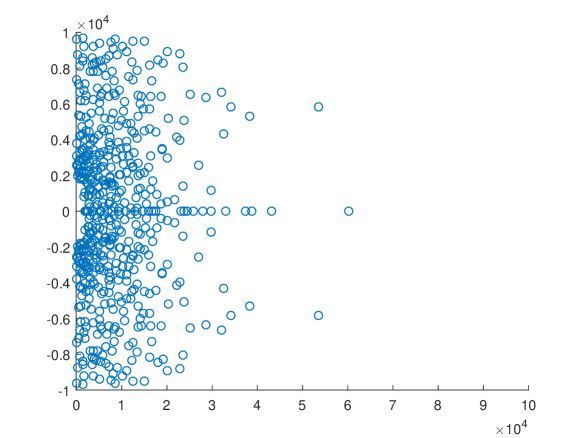
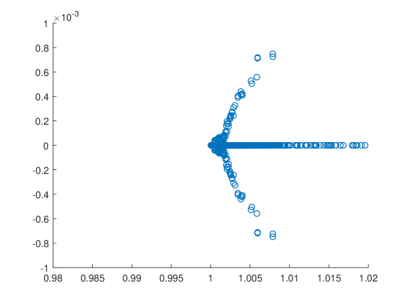
Figure 1: Matrices $A$ and $B$ are from Example 1 in Section 5. Left: Spectrum of original problem. Right: Spectrum after Cayley transformation.

2.3 Arnoldi Method for Linear Systems

The computation cost can be significantly reduced by exploiting (14). Consider the orthogonal projection method for

$$M{\boldsymbol{x}}={\boldsymbol{b}}.$$

Let the initial guess be ${\boldsymbol{x}}_{0}={\boldsymbol{0}}$. One seeks an approximate solution ${\boldsymbol{x}}_{m}$ in $K_{m}(M;{\boldsymbol{b}})$ of dimension $m$ by imposing the Galerkin condition [10]

$$({\boldsymbol{b}}-M{\boldsymbol{x}}_{m})\perp K_{m}(M;{\boldsymbol{b}}).$$ (15)

The basic Arnoldi’s process (Algorithm 6.1 of [11]) is as follows.

• Choose a vector ${\boldsymbol{v}}_{1}$ of norm $1$

• for $j=1,2,\ldots,m$

  • $h_{ij}=(M{\boldsymbol{v}}_{j},{\boldsymbol{v}}_{i}),\quad i=1,2,\ldots,j$,

  • ${\boldsymbol{w}}_{j}=M{\boldsymbol{v}}_{j}-\sum_{i=1}^{j}h_{ij}{\boldsymbol{v}}_{i}$,

  • $h_{j+1,j}=\|{\boldsymbol{v}}_{j}\|_{2}$, if $h_{j+1,j}=0$ stop

  • ${\boldsymbol{v}}_{j+1}={\boldsymbol{w}}_{j}/h_{j+1,j}$.

Let $V_{m}$ be the $n\times m$ orthogonal matrix with column vectors ${\boldsymbol{v}}_{1},\ldots,{\boldsymbol{v}}_{m}$ and $H_{m}$ be the $m\times m$ Hessenberg matrix whose nonzero entries $h_{i,j}$ are defined as above. From Proposition 6.6 of [11], one has that

$$MV_{m}=V_{m}H_{m}+{\boldsymbol{v}}_{m+1}{h}_{m+1,m}{\boldsymbol{e}}^{T}_{m}$$ (16)

such that

$$\text{span}\{\mathrm{col}(V_{m})\}=K_{m}(M;{\boldsymbol{b}}).$$

Let ${\boldsymbol{x}}_{m}=V_{m}{\boldsymbol{y}}$. The Galerkin condition (15) becomes

$$V^{T}_{m}{\boldsymbol{b}}-V^{T}_{m}MV_{m}{\boldsymbol{y}}={\boldsymbol{0}}.$$ (17)

Since $V_{m}^{T}MV_{m}=H_{m}$ (see Proposition 6.5 of [10]), the following holds:

$$H_{m}{\boldsymbol{y}}=V^{T}_{m}{\boldsymbol{b}}.$$

From the construction of $V_{m}$, ${\boldsymbol{v}}_{1}=\dfrac{{\boldsymbol{b}}}{\|{\boldsymbol{b}}\|_{2}}$. Let $\beta=\|{\boldsymbol{b}}\|_{2}$. Then

$${\boldsymbol{y}}=\beta H_{m}^{-1}{\boldsymbol{e}}_{1}.$$ (18)

Consequently, the residual of the approximated solution ${\boldsymbol{x}}_{m}$ can be written as

$$\|{\boldsymbol{b}}-M{\boldsymbol{x}}_{m}\|_{2}={h}_{m+1,m}|{\boldsymbol{e}}_{m}^{T}{\boldsymbol{y}}|.$$ (19)

Due to the shift invariant property, one has that

$$\{I+(\sigma-z)M\}V_{m}=V_{m}(I+(\sigma-z)H_{m})\\ +(\sigma-z){\boldsymbol{v}}_{m+1}{h}_{m+1,m}{\boldsymbol{e}}^{T}_{m}.$$ (20)

By imposing a Galerkin condition similar to (15), we have that

$$V^{T}_{m}{\boldsymbol{b}}-V^{T}_{m}\{I+(\sigma-z)M\}V_{m}{\boldsymbol{y}}=0,$$ (21)

which implies

$$\{I+(\sigma-z)H_{m}\}{\boldsymbol{y}}=\beta{\boldsymbol{e}}_{1}.$$ (22)

From (19), one has that

$$\|b-\{I+(\sigma-z)M\}{\boldsymbol{x}}_{m}\|_{2}=(\sigma-z){h}_{m+1,m}|{\boldsymbol{e}}_{m}^{T}{\boldsymbol{y}}|.$$ (23)

Matrix $M$ is an $n\times n$ matrix and $H_{m}$ is an $m\times m$ upper Hessenberg matrix such that $m\ll n$. Once $H_{m}$ and $V_{m}$ are constructed by Arnoldi’s process, they can be used to solve (22) for different $z$’s with residual given by (23). The residual can be monitored with a little extra cost.

Next we explain how the Arnoldi’s process is incorporated in RIM. To solve (8) for quadrature points $z_{j}$’s, one chooses a proper shift $\sigma$. Following (14), one has that

$$(I+(\sigma-z_{j})M){\boldsymbol{x}}_{j}={\boldsymbol{b}},$$ (24)

where $M=(A-\sigma B)^{-1}B$ and ${\boldsymbol{b}}=(A-\sigma B)^{-1}{\boldsymbol{f}}$.

From (20) and (22),

$${\boldsymbol{y}}_{j} = \beta(I+(\sigma-z_{j})H_{m})^{-1}{\boldsymbol{e}}_{1},$$ (25)

$${\boldsymbol{x}}_{j} \approx V_{m}{\boldsymbol{y}}_{j},$$

$$P{\boldsymbol{f}} \approx \dfrac{1}{2\pi i}\sum w_{j}V_{m}{\boldsymbol{y}}_{j}.$$ (26)

Hence the Krylov subspace for $M=(A-\sigma B)^{-1}B$ can be used to solve many linear systems associated with $z_{j}$’s close to $\sigma$.

3 An Efficient Indicator

Another critical problem of RIM is to how to define the indicator $\delta_{S}$. As seen above, the indicator in [2] defined by (7) is to project a random vector twice. One needs to solve linear systems with different right hand sides, i.e., ${\boldsymbol{f}}$ and $P{\boldsymbol{f}}/|P{\boldsymbol{f}}|$. Consequently, two Krylov subspaces, rather than one, are constructed for a single shift $\sigma$.

In this section, we propose a new indicator that avoids the construction of two Krylov subspaces. The indicator stills needs to resolve the two problems (P1 and P2) in Section 1. The idea is to approximate $|P{\boldsymbol{f}}|$ with different sets of trapezoidal quadrature points by taking the advantage of the Cayley transformation and Arnoldi’s method discussed in the previous section.

Let $P{\boldsymbol{f}}|_{n}$ be the approximation of $P{\boldsymbol{f}}$ with $n$ quadrature points. It is well-known that trapezoidal quadratures of a periodic function converges exponentially [14, Section 4.6.5], i.e.,

$$\left|P{\boldsymbol{f}}-P{\boldsymbol{f}}|_{n}\right|=O(e^{-Cn}),$$

where C is a constant depending on ${\boldsymbol{f}}$. The spectral projection satisfies

$$P{\boldsymbol{f}}|_{n}\begin{cases}\neq{\boldsymbol{0}}&\text{if there are eigenvalues inside }S,\\ \approx{\boldsymbol{0}}&\text{no eigenvalue inside }S.\end{cases}$$

For a large enough $n_{0}$, one has that

$$\dfrac{\left|P{\boldsymbol{f}}|_{2n_{0}}\right|}{\left|P{\boldsymbol{f}}|_{n_{0}}\right|}=\begin{cases}\dfrac{|P{\boldsymbol{f}}|+O(e^{-C2n})}{|P{\boldsymbol{f}}|+O(e^{-Cn})}&\text{if there are eigenvalues inside }S,\\ \dfrac{O(e^{-C2n})}{O(e^{-Cn})}=O(e^{-Cn})&\text{no eigenvalue inside }S.\end{cases}$$

The new indicator is set to be

$$\delta_{S}={|P{\boldsymbol{f}}_{2n_{0}}|}/{|P{\boldsymbol{f}}_{n_{0}}|}.$$ (27)

A threshold value $\delta_{0}$ is also needed to decide if there exists eigenvalue in $S$ or not. If $\delta_{S}>\delta_{0}:=0.2$, $S$ is said to be admissible, i.e., there exists eigenvalue(s) in $S$. The value $0.2$ is chosen based on numerical experimentation. Due to (25) - (26), the computation cost to evaluate the new indicator is not expensive.

4 The New Algorithm

Now we are ready to give the algorithm in detail. It starts with several shifts $\sigma$’s distributed in $S$ uniformly. The associated Krylov subspaces $K_{m}(M;{\boldsymbol{b}})$ are constructed and stored. For a quadrature point $z$, the algorithm first attempts to solve the linear system (9) using the Krylov subspace with shift $\sigma$ closest to $z$. If the residual is larger than the given precision $\epsilon$, a Krylov subspace with a new shift $\sigma$ is constructed, stored and used to solve the linear system. Briefly speaking, the algorithm constructed some Krylov subspaces with different $\sigma$’s. These subspaces are then used to solve the linear system for all quadrature points $z_{j}$’s. From (25) and (26), instead of solving a family of linear systems of size $n$, the algorithm solves linear systems of reduced size $m$ for most $z_{j}$’s. This is the key idea to speed up RIM. We denote this improved version of RIM by RIM-C (RIM with Cayley transformation).

Given a search region $S$ and a normalized random vector ${\boldsymbol{f}}$, we compute the indicator $\delta_{S}$ using (27). Without loss of generality, $S$ is assumed to be a square. We set $n_{0}=4$ in (27). If $\delta_{S}>0.2$, $S$ is divided uniformly into $4$ regions. The indicators of these regions are computed. This process continues until the size of the region is smaller than $d_{0}$.

1. Algorithm RIM-C:

2. RIM-C$(A,B,S,{\boldsymbol{f}},d_{0},\epsilon,\delta_{0},m,n_{0})$

3. Input:

   • $A,B$: $n\times n$ matrices

   • $S$: search region in $\mathbb{C}$

   • ${\boldsymbol{f}}$: a random vector

   • $d_{0}$: precision

   • $\epsilon$: residual threshold

   • $\delta_{0}$: indicator threshold

   • $m$: size of Krylov subspace

   • $n_{0}$: number of quadrature points

4. Output:

   • generalized eigenvalues inside $S$

1. Choose several $\sigma$’s uniformly in $S$ and construct Krylov subspaces

2. Compute $\delta_{S}$ using (27).

   • Let $z$ be a quadrature point.

   • Check if the linear system can be solved using the existing Krylov subspaces with residual less than $\epsilon$.

   • Otherwise, choose a new $\sigma$, construct a new Krylov subspace to solve the linear system.

3. Decide if each $S$ contains eigenvalues(s).

   • If $\delta_{S}=\dfrac{|P{\boldsymbol{f}}|_{2n_{0}}|}{|P{\boldsymbol{f}}|_{n_{0}}|}<\delta_{0}$, exit.

   • Compute the size of $S$, $h(S)$.

   • If $h(S)>\epsilon_{0}$, uniformly partition $S_{i}$ into subregions $S_{j},j=1,\ldots 4$

     • for $j=1$ to $4$

     • call RIM-C$(A,B,S_{j},{\boldsymbol{f}},d_{0},\epsilon,\delta_{0},m,n_{0})$

     • end

   • Otherwise, output the eigenvalue $\lambda$ and exit.

5 Numerical Examples

In this section, RIM-C (implemented in Matlab) is employed to compute all the eigenvalues in a given region. To the authors’ knowledge, there exists no eigensolver doing exactly the same thing. We compare RIM-C with ‘eigs’ in Matlab (IRAM: Implicitly Restarted Arnoldi Method [12]). Although the comparison seems to be unfair to both methods, it gives some idea about the performance of RIM-C.

The matrices for Examples 1-5 come from a finite element discretization of the transmission eigenvalue problem [7, 3] using different mesh size $h$. Therefore, the spectra of these problems are similar. For Matlab function ‘eigs(A,B,K,SIGMA)’, ‘K’ and ‘SIGMA’ denote the number of eigenvalues to compute and the shift, respectively. For RIM-C, the size of Krylov space is set to be $m=50$, $d_{0}=10^{-9}$, $\epsilon=10^{-10}$, $\delta_{0}=0.2$, and $n_{0}=4$. All the examples are computed on a Macbook pro with 16 Gb memory and 3 GHz Intel Core i7.

Example 1: The matrices $A$ and $B$ are $1018\times 1018$ (mesh size $h\approx 0.1$). The search region $S=[1,11]\times[-1,1]$. For ‘eigs’, the ‘shift’ is set to be $5.5$. For this problem, it is known that there exist $5$ eigenvalues in $S$. Therefore, ‘K’ is set to be $5$. Note that RIM-C does not need this information. The results are shown in Table 1. Both RIM-C and ‘eigs’ compute $5$ eigenvalues and they are consistent. ‘eigs’ uses less time than RIM-C.

Table 1: Eigenvalues computed and CPU time by RIM-C and ‘eigs’ for Example 1.

	RIM-C	‘eigs’
Eigenvalues	3.994539018848445	3.994539018856096
	6.939719143800903	6.939719143804773
	6.935053985873570	6.935053985844678
	10.654665853490588	10.654665853441946
	10.658706024650019	10.658706024609756
CPU time	0.284922s	0.247310s

Example 2: Matrices $A$ and $B$ are $4066\times 4066$ (mesh size $h\approx 0.05$). Let $S=[20,30]\times[-6,6]$. For ‘eigs’, ‘shift’ is set to be $25$. Again, it is known in advance that there are $3$ eigenvalues in $S$. Hence ‘K’ is set to be $3$. The results are shown in Table 2. Both methods compute same eigenvalues and ‘eigs’ is faster.

Table 2: Eigenvalues computed and CPU time by RIM-C and ‘eigs” for Example 2.

	RIM-C	‘eigs’
Eigenvalues	23.803023938395199	23.803023938403236
	$\pm$ 5.682304314876092i	$\qquad\pm$ 5.682304314840053i
	24.737027497006540	24.737027497003453
	24.750959635036583	24.750959635022376
	25.278145187465789	25.278145187457707
	25.284501515028143	25.284501515036474
CPU time	0.558687s	0.333513s

Example 3: Matrices $A$ and $B$ are $16258\times 16258$ matrices (mesh size $h\approx 0.025$). Let $S=[0,20]\times[-6,6]$. There are $10$ eigenvalues in $S$. It is well-known that the performance of ‘eigs’ is highly dependent on ‘shift’. In Table 3, we show the time used by RIM-C and ‘eigs’ with different shifts ‘shift =5, 10, 15’. Notice that when the shift is not good, ‘eigs’ uses much more time. In practice, good shifts are not known in advance.

Table 3: CPU time used by RIM and ‘eigs’ with different shifts for Example 3.

	RIM-C	‘eigs’ shift=5	‘eigs’ shift=10	‘eigs’ shift=15
CPU time	2.571800s	0.590186	7.183679s	0.392902s

Example 4: We consider a larger problem: $A$ and $B$ are $260098\times 260098$. Let $S=[0,20]\times[-6,6]$ (mesh size $h\approx 0.00625$). There are $17$ eigenvalues in $S$. The results are in Table 4. This example, again, shows that for larger problems without any spectrum information, the performance of RIM-C is quite stable and consistent. However, the performance of ‘eigs’ varies a lot with different ‘shifts’.

Table 4: CPU time used by RIM and ‘eigs’ with different shifts for Example 4.

	RIM-C	‘eigs’ shift=5	‘eigs’ shift=10
CPU time	104.228413s	1696.703477s	272.506573s

Example 5: This example demonstrates the effectiveness and robustness of the new indicator. The same matrices in Example 3 ($16258\times 16258$) are used. Consider three regions $S_{1},S_{2}$ and $S_{3}$. $S_{1}=[18.4,18.8]\times[-0.2,0.2]$ has one eigenvalue inside. $S_{2}=[14.6,14.8]\times[-0.1,0.1]$ has two eigenvalues inside. $S_{3}=[19.7,19.9]\times[-0.1,0.1]$ contains no eigenvalue. Table 5 shows the indicators of these three regions computed using (27). It is seen that the indicator is different when there are eigenvalues inside the region and when there are no eigenvalues.

Table 5: Indictors: $S_{1}$ and $S_{2}$ contain at least one eigenvalue, $S_{3}$ contains no eigenvalue.

number of quadrature points	$P{\boldsymbol{f}}_{S_{1}}$	$P{\boldsymbol{f}}_{S_{2}}$	$P{\boldsymbol{f}}_{S_{3}}$
4	0.021036161440	0.000256531878	0.001173702609
8	0.020981705584	0.000258504259	0.000044238403
$\delta_{S}$	0.997411	0.992370	0.037691

Table 6 shows the means, minima, maxima, and standard deviations of indicators of these three regions computed using $100$ random vectors. The indicators are consistent for different random vectors.

Table 6: Means, minima, maxima, and standard deviations of indicators using $100$ random vectors.

$S$	mean	min.	max.	std. dev.
$S_{1}$	0.99848393687	0.66250246918	1.43123449889	0.08740952445
$S_{2}$	0.99926772105	0.92600650392	1.14648387384	0.01788832121
$S_{3}$	0.03763601782	0.03734608324	0.03775912970	0.00010228556

Example 6: The last example shows the potential of RIM-C to treat large matrices. The sparse matrices are of ${\bf 15,728,640\times 15,728,640}$ arising from a finite element discretization of localized quantum states in random media [1]. RIM-C computed $136$ real eigenvalues in $(2,3)$, shown in the right picture of Fig. 2.

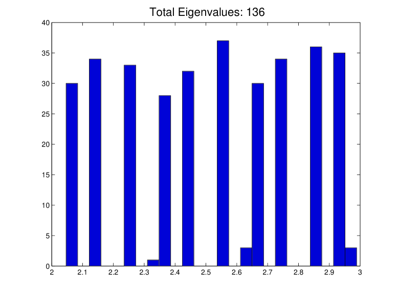
Figure 2: Distribution of eigenvalues in $(2,3)$ for Example 6.

6 Conclusions and Future Works

This purposes of this paper is to compute (all) the eigenvalues of a large sparse non-Hermitian problem in a given region. We propose a new eigensolver RIM-C, which is an improved version of the recursive integral method using spectrum projection. RIM-C uses Cayley transformation and Arnoldi method to reduce the computation cost.

To the authors’ knowledge, RIM-C is the only eigensolver for this particular purpose. As we mentioned, the comparison of RIM-C and ‘eigs’ is unfair to both methods. However, the numerical results do show that RIM-C is effective and has the potential to treat large scale problems.

Currently, the algorithm is implemented in Matlab. A parallel version using C++ is under development. For the time being, RIM-C only computes eigenvalues, which is good enough for some applications. However, adding a component to give the associated eigenvectors is necessary for other applications. It would also be useful to provide the multiplicity of an eigenvalue. These are our future works to make RIM-C a robust efficient eigensolver.

References

- [1] D.N. Arnold, G. David, D. Jerison, S. Mayboroda and M. Filoche, Effective confining potential of quantum states in disordered media. Physical Review Letters, 116(5), 2016, 056602.
- [2] R. Huang, A. Struthers, J. Sun and R. Zhang, Recursive integral method for transmission eigenvalues. Journal of Computational Physics, Vol. 327, 830 - 840, 2016.
- [3] J. Sun, Iterative methods for transmission eigenvalues. SIAM J. Numer. Anal., 49(5),1860-1874, 2011.
- [4] E. Polizzi, Density-matrix-based algorithms for solving eigenvalue problems. Phys. Rev. B., 79, 115112, 2009.
- [5] T. Sakurai and H. Sugiura, A projection method for generalized eigenvalue problems using numerical integration. J. Comput. Appl. Math, 159(1), 119-128, 2003.
- [6] G.H. Golub and H.A. van der Vorst, Eigenvalue computation in the 20th century. J. Comput. Appl. Math, 123(1-2), 35-65, 2000.
- [7] X. Ji, J. Sun and T. Turner, A mixed finite element method for Helmholtz Transmission eigenvalues. ACM Trans. Math. Software, 38(4), Article No. 29, 2012.
- [8] S. Boccaletti, V. Latora, Y. Moreno, M. Chavez, D.U. Hwang, Complex Networks: Structure and Dynamics. Physics Reports, 424(4-5), 175-308, 2006.
- [9] K. Meerbergen, The Solution of Parametrized Symmetric Linear Systems. SIAM Journal on Matrix Analysis and Applications, 24(4),1038-1059, 2003.
- [10] Y. Saad, Iterative Methods for Sparse Linear Systems, 2nd Ed., Society for Industrial and Applied Mathematics, 2003.
- [11] Y. Saad, Numerical Methods for Large Eigenvalue Problems, 2nd Ed., Society for Industrial and Applied Mathematics, 2011.
- [12] R.B. Lehoucq, D.C. Sorensen and C. Yang, ARPACK User’s Guide – Solution of Large-Scale Eigenvalue Problems with Implicitly Restarted Arnoldi Methods, Society for Industrial and Applied Mathematics, Philadelphia, PA, 1998.
- [13] J. Sun and A. Zhou, Finite Element Methods for Eigenvalue Problems, Chapman and Hall/CRC, 2016.
- [14] P.J. Davis and P. Rabinowitz, Methods of Numerical Integration, 2nd Ed., Academic Press, Inc., Orlando, FL, 1984.