Emerging Dynamics Arising From Coarse-Grained Quantum Systems
Abstract
The purpose of physics is to describe nature from elementary particles all the way up to cosmological objects like cluster of galaxies and black holes. Although a unified description for all this spectrum of events is desirable, an one-theory-fits-all would be highly impractical. To not get lost in unnecessary details, effective descriptions are mandatory. Here we analyze what are the dynamics that may emerge from a full quantum description when one does not have access to all the degrees of freedom of a system. More concretely, we describe the properties of the dynamics that arise from quantum mechanics if one has only access to a coarse grained description of the system. We obtain that the effective maps are not necessarily of Kraus form, due to correlations between accessible and non-accessible degrees of freedom, and that the distance between two effective states may increase under the action of the effective map. We expect our framework to be useful for addressing questions such as the thermalization of closed quantum systems, as well as the description of measurements in quantum mechanics.
pacs:
03.65.Ta, 03.67.-a, 03.65.YzI Introduction
It is widely accepted that quantum mechanics provides currently the best desciption we have of the physical world. However, the description of systems in our daily lives does not require the whole framework arising from quantum mechanics. In fact, our everyday life experiences heavily rely on effective (macroscopic) descriptions which are far less complex than their underlying intricate quantum characterization. For example, to describe the behavior of a macroscopic object, like the thermal expansions or compressions of a rail line, we do not need to specify the quantum states of all atoms composing such an object. In this situation we resort to the theory of thermodynamics Callen (1985), which is probably the clearest example of effective theories. Although the systems treated within this theory are composed by many quantum interacting particles, macroscopic variables –such as temperature, volume, and pressure– describe the systems well enough, allowing, for instance, for the design of thermal machines.
The idea of different scales is central in physics. But, how does the description in one scale emerge from the description in a deeper scale? Different ways of coarse graining the description of a system are often employed Zwanzig (1961); Mori (1965); Castiglione et al. (2008); Gell-Mann and Hartle (2014); Grabert (1982) in order to “zoom out” from one level and obtain an effective description. Coarse grainings frequently appear in statistical physics Grabert (1982), and are arguably the central tool in the renormalization method developed by Kadanoff and Wilson Kadanoff (1966); Wilson (1975). Nevertheless, some of these early methods are sometimes based on not so well controlled approximations or on projections, leading thus to ill-defined and/or probabilistic effective dynamics when applied to quantum systems.
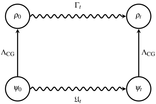
In the last decades, with the birth of the quantum information field, various tools were developed to deal with many-body quantum systems Nielsen and Chuang (2000). In particular, the theory of completely positive linear maps Watrous (2006); Wilde (2017); Wolf (2012), which aims at describing the most general transformations that can be applied to a system (including the most general time evolution), became well established. This has been accompanied and supported by the formalization and development of a theory for quantum correlations Horodecki et al. (2009), and by efficient descriptions of many-body quantum states Perez-Garcia et al. (2007); Orús (2014). The goal of the present contribution is to employ some of these tools in order to obtain effective descriptions of quantum systems and their dynamics. More concretely, see Fig. 1, given a system in the state represented by a density operator evolving by the unitary map ; what is the dynamics induced by a coarse graining ? What types of dynamics might emerge when we departure from a full quantum description of the systems?
In what follows we present a framework to address these questions. Its construction is closely related to that of open quantum systems Breuer and Petruccione (2002); Carteret et al. (2008); Štelmachovič and Bužek (2001); Ángel Rivas et al. (2014). In fact, concepts like the correlation between system and environment, and maps divisibility will play an important role here as well. Nevertheless, our framework encompasses and generalizes this previous formalism, as ours can be used in many other situations. It can, for instance, be used to describe closed systems from which just partial information is available, what might play a significant role in the thermalization of closed quantum systems Eisert et al. (2015); Faist (2016). Our work is also related to recent articles by Kofler and Brukner Kofler and Brukner (2007, 2008). In these articles the authors analyze the effect of coarse-grained measurements in order to explain the emergence of the classical word. Their approach, however, is not dynamical, and that is exactly the gap we want to fill out.
Our article is organized as follows: In Section II we introduce two different characterizations of completely positive and trace preserving (CPTP) linear maps, which will allow us to describe generalized quantum dynamics and the coarse graining maps. In this contribution, a coarse graining map will simply be a CPTP linear map that reduces the dimension of the system. Such maps were recently used to obtain a sufficient criteria for the entanglement of high-dimensional bipartite states Saideh et al. (2016). After that, in Section III, we obtain the effective dynamics induced by the coarse graining , underlying evolution , and initial state . The properties of the effective map are discussed in Section IV. In Section V we show that the distance between two effective states may increase under the action of the same effective map . This is in contrast with the usual contractive property of CPTP linear maps Nielsen and Chuang (2000). Finally, in Section VI we draw some final conclusions and hint to some possible applications of the developed formalism.
II CPTP linear maps: general dynamics and coarse graining
In order to define the coarse graining operations, which are the ones we are interested here, we will first briefly review some properties of CPTP linear maps. Comprehensive expositions can be found, for example, in Watrous (2006); Wilde (2017); Wolf (2012); Nielsen and Chuang (2000).
Let be the Hilbert space assigned to a -dimensional quantum system. We define as the set of all linear operators acting on , and the convex set containing all the possible states of the system. Let be a linear map which abides by two constraints: i) it is trace preserving, meaning that we have ; and ii) it is completely positive, i.e., for all positive operators , with an arbitrary finite dimensional Hilbert space, the linear map is such that Wolf (2012). The first imposition guarantees that probabilities are conserved through the map action, while the completely positivity condition ensures that states are mapped into states even if the map acts only on a subsystem of the whole system. The following well-known theorem gives a very useful characterization of CPTP linear maps.
Theorem 1 (Nielsen and Chuang (2000); Wolf (2012)).
A linear map is completely positive and trace-preserving if and only if there exists a finite set of linear operators , with each known as a Kraus operator, such that :
It is worth noticing that CPTP linear maps generalize the evolution of a quantum system, with the unitary evolution being a particular linear map with a single Kraus operator, namely the unitary itself. In general, the number of Kraus operators is unlimited, but it is always possible to characterize a CPTP linear map with a set of Kraus operators with at most elements Nielsen and Chuang (2000), as this is the number of generators for the map. Moreover, the set of Kraus operators describing a given CPTP linear map is not unique. Given the two sets and , with , they represent the same CPTP linear map if, and only if, there exists a unitary such that (where, if necessary, we pad the smallest set with zeros) Nielsen and Chuang (2000); Wolf (2012).
This more general type of evolution allows for describing processes where there is a loss of information about the system, with pure states evolving to mixed ones. That is the case, for instance, when one is dealing with open quantum systems Breuer and Petruccione (2002).
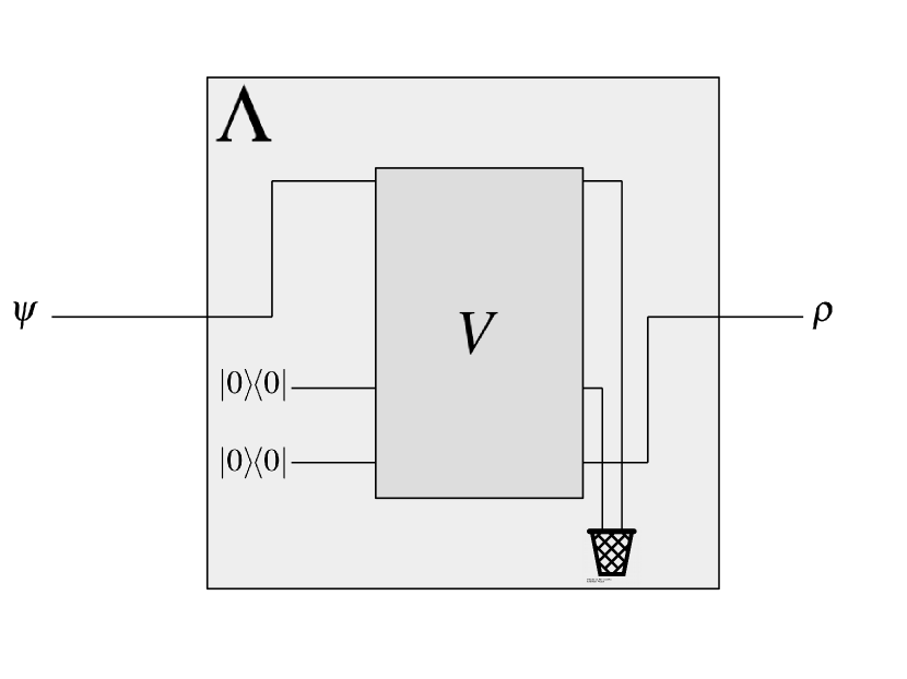
For the coarse graining operations we are going to employ below, the following (see Fig. 2) operational way to describe CPTP linear maps will turn handy.
Theorem 2 (Wolf (2012)).
Let be a CPTP linear map. Then there exists an auxiliary Hilbert space , with dimension , and a unitary acting on such that
Operationally, this theorem means that we can interpret CPTP linear maps as a unitary interaction among three systems, and further discarding of the first two parties. See Fig. 2. This interpretation is reminiscent of open quantum systems, where the system interacts unitarily with the environment, with the latter being discarded as we have no control about, or interest in, it. Here, however, the roles of system and environment are not so well delineated. As we want to allow for maps with different input-output dimensions, the partial trace is taken over the auxiliary system and also over the factor encoding the initial system state.
The theorems above provide equivalent characterization of CPTP linear maps, hence we will use them interchangeably. In fact, it is easy to relate them by setting . This connection shows that the auxiliary system is necessary as to accommodate CPTP linear maps which require a number of Kraus operators bigger than . We should stress that for a CPTP linear map with a set of Kraus operators , we take the dimension of as , and must find an equivalent set of Kraus operators with elements, . Hence, whenever the auxiliary dimension will be greater than one.
We are finally in position to establish the coarse graining operations. Roughly speaking, descriptions are named coarse-grained when some fine details of the underlying model are smoothed out, or replaced by average behaviors. In order to get valid descriptions of states after the coarse graining, we define it as a CPTP linear map that reduces the dimension of the system:
When one is not able to resolve the system in full detail, the coarse graining map gives an effective state for the system.
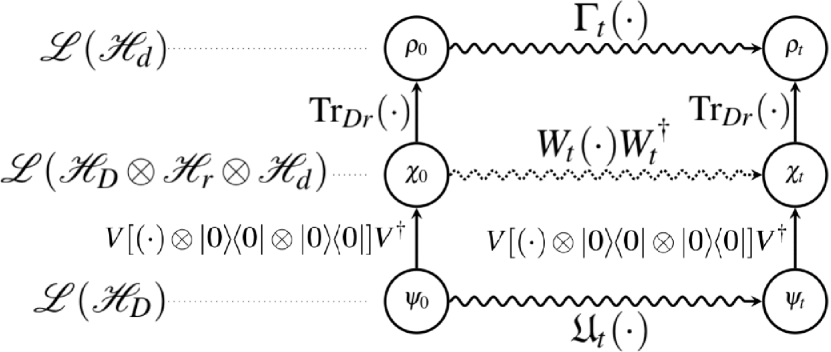
Resorting to the characterization of CPTP linear maps in Theorem 2, we know that there exists an auxiliary space and a unitary , such that
Operationally, what the unitary accomplishes is to "write" the accessible degrees of freedom into the party in , while the unaccessible degrees of freedom are left in to be later discarded. See Fig. 3. The intermediate states and , which live in , are virtual states, in the sense that they are mathematical abstractions. In this level the two contributions of degrees of freedom, accessible and non-accessible are split, but may be correlated.
II.1 Example: a blurred and saturated detector
In order to give a concrete example, let us consider a typical optical lattice experiment herson et al. (2010); Fukuhara et al. (2015); Preiss et al. (2015). In these experiments a periodic oscillating potential is constructed by counter-propagating light beams, and individual atoms are trapped in each potential minimum. In the deep Mott insulator regime two hyperfine levels of each atom act as a qubit, and neighboring qubits interact with each other via a Heisenberg-like Hamiltonian. The measurement of each atom is made via a fluorescence technique: the atoms are shone with a laser in way that if an atom is in the state, say, , light is scattered by the atom, whereas if its state is no light is scattered. To resolve the light coming from each atom a powerful lens is necessary, and only recently a single-atom resolution was accomplished Kuhr (2016).
To simplify, consider the case with only two atoms. Suppose that the lens available is not good enough as to resolve the light coming from each individual atom. In this situation the states and cannot be distinguished. Moreover, imagine that the amount of light coming from a single atom is already sufficient to saturate the detector. Then, having two excitations, , or one excitation, or , leads to the same signal. In such conditions to describe the experiment with two atoms is superfluous, and an effective description becomes handy. These experimental conditions suggest the coarse graining presented in Table 1.
Note that as the detector does not distinguish between the states , , and there can be no coherence in this subspace. Furthermore, the factors are necessary to make a CPTP linear map. This signals that coherences in the effective description might decrease, but they do not necessarily vanish Faist (2016). This can be readily seen by evaluating the action of over a general two-qubits pure state , with , which gives:
This effective state accounts for the statistics of all possible measurements that can be carried out by the detector here modeled. It is thus the description that really matters for this experimental condition, not carrying unaccessible information.
The Kraus operators for this map can be easily obtained by a quantum process tomography Nielsen and Chuang (2000), and are given by:
As we have four Kraus operators, , and the dimension of the underlying system is also four, , then the auxiliary system in can be taken as 1-dimensional and as such can be ignored. With the above Kraus operators, and neglecting the system in , one can immediately obtain the corresponding unitary for this example:
III Coarse Graining Induced Dynamics
Now we address the central question of this contribution: what are the dynamics that might emerge from a fully quantum description if we are not able to resolve the system in all its details? More concretely, we look for an effective map which makes the diagram in Fig. 1 consistent, i.e, in a way that , with . The induced dynamics then emerges from a coarse grained description of the underlying dynamics.
To obtain the induced dynamics acting on the effective state , we generalize the procedure suggested by Štelmachovič and Bužek in Štelmachovič and Bužek (2001). There they proposed to write the state of the system and environment as the tensor product of its local parts plus a correlation term. Despite the fact that here we do not have such a splitting between system and environment, the action of the unitary , see Fig. 3, suggests the following decomposition:
| (1) |
where , , . Note that is a state in . Equation (1) is equivalent to Štelmachovič and Bužek decomposition in the abstract level , with the last term now representing the correlation between the degrees of freedom which can be accessed and those that cannot. As is unitary, we can equivalently write:
| (2) |
From the left hand side of Eq. (2) we get the evolved effective state by applying the underlying evolution map onto the first tensor factor, followed by the application of and further partial trace of the two first tensor factors:
The last equality comes from demanding consistence of the diagram in Fig. 1. Accordingly, assuming the underlying evolution map of the form , from the right hand side of Eq. (1) we get the effective evolution:
| (3) |
where is the unitary evolution operator in the level , i.e., . See Fig 3.
The above evolution equation can be rewritten in a more meaningful way as
| (4) |
with , where we employed the spectral decomposition . This is the dynamics that emerges if one is not able, or does not wish, to resolve all the details of the underlying system.
The expression in Eq. (4) is composed by two contributions: the first one displays a Kraus form (see Theorem 1), with the corresponding set of effective Kraus operators; the second one represents the evolution of the correlations between accessible and non-accessible degrees of freedom. This second term can be more clearly appreciated by evoking the Bloch representation of :
| (5) | ||||
where is a vector whose components are the generalized Pauli matrices, is the Bloch vector of , is the Bloch vector of , and the coefficients fix the correlation between accessible and non-accessible degrees of freedom. Defining the correlation matrix , the evolution of the coarse grained state can be written as:
| (6) |
It can be easily verified that , and that as is unitary and the (generalized) Pauli matrices are traceless. These conditions guarantee that for all times. The structure of this type of evolution is very similar to the one describing open quantum systems when system and environment are initially correlated Carteret et al. (2008); Štelmachovič and Bužek (2001).
III.1 Example: effective dynamics as seen by a blurred and saturated detector
Consider again the situation described in subsection II.1: two atoms in neighboring wells of an optical lattice being observed by a blurred and saturated detector. Suppose now that the atoms interact as specified by the Hamiltonian , with a coupling constant in units of frequency. In such situation, an initial two-qubit pure state evolves to:
The evolution of the effective state can then be easily evaluated via , to give:
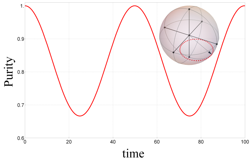
As a concrete example, the effective evolution of a state with all coefficients equal, for , is shown in the inset of Fig. 4. Figure 4 also shows how the purity, , oscillates with time, exhibiting the alternation between pure and mixed state in the effective level. This is in clear contrast with the complete description of the system, where the system is pure for all times.
It is interesting to notice that the coefficients of define the state , but also enter in the definition of the effective map . In the above example this can be verified by evaluating , which will also depend on the coefficients . That in turn, means that the effective Kraus operators will also change with the – thus by changing the map may change. The same is true for the correlation matrix . This interdependence of the parameters is treated in the next section, where the properties of are analyzed.
IV Properties of
The effective map is generated by the underlying evolution , the coarse graining map , and the state . Equation (6), however, does not make explicit how the map depends on the elemental state . For instance, how do we change the effective map for a fixed input state ? Or, how to change the effective input state keeping fixed? In what follows we address these and other questions making use of the Bloch representation for :
| (7) |
where is the Bloch vector of .
IV.1 Fix , change
Fixed the coarse graining map, the Bloch vector of is obtained from by the linear relations:
| (8) |
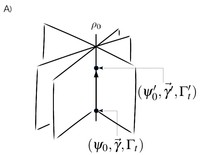
In the dimensional space of Bloch vectors of , these constraints represent hyperplanes whose intersection depicts the effective state . It is important to notice that since , the set of linear equations for the coefficients is under-determined, meaning that various states lead to the same effective state . Geometrically, in the “-space”, this many-to-one mapping is visualized as an hyper-surface of possible solutions.
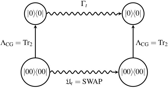
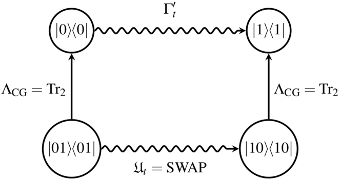
Now, with this geometric perspective in mind, a fixed coarse graining and a fixed underlying evolution, it can be seem that changes in , that move parallel to the hyper-planes within the solution hyper-surface will not affect the effective state . Nevertheless, such change can induce modifications in or in , and as such will change. A simple example is presented in Fig. 5, and an abstract representation of the -space and the change in can be seen in Fig. 6.
 |
 |
 |
 |
IV.2 Fix , change : the domain of
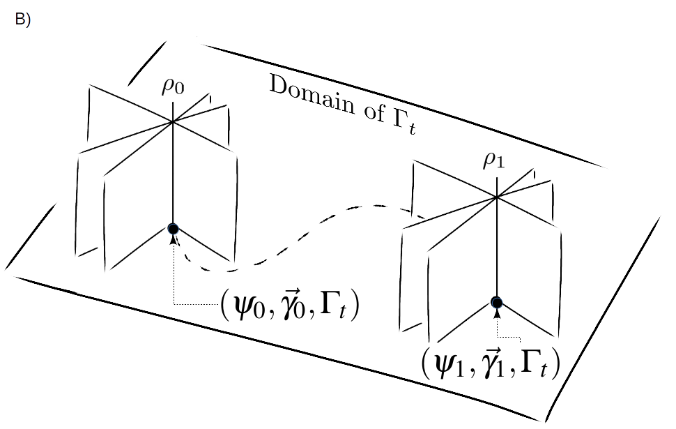
To change the effective state we must change the value of the ’s. Geometrically this is represented by moving the hyperplanes, defined in Eq. (8), in the -space. After the hyper-planes displacement, a new intersection is obtained representing now another effective state, say, . As moving parallel to the hyper-planes changes the map, this time we must move perpendicular to the hyper-planes. This guarantees that only the effective state is changing. See Fig. 6A).
It is important to notice that this change might in fact modify or . This, however, comes only because of the change in the effective input state, as these quantities might be functions of . Putting it differently, the effective Kraus operators might change, but this is only due to the change in the input of the effective map . The dynamical equation (6) can be rewritten as to make this dependence explicit:
| (9) |
where .
We can now determine the domain of a given . An effective map is generated by an elemental state , an underlying evolution map , and a coarse graining map . This information already gives the first element in the domain of , namely, . The coarse graining fixes the hyper-planes in the -space through Eq.(8). Let be the normal vector for the -th hyper-plane, and be the Bloch vector of . The domain of is then given by all generated from with Bloch vector for which there exists coefficients such that . The latter condition guarantees that the Bloch vector of all states in the domain of can be reached from by moving it perpendicular to the hyper-planes in Eq. (8), and as such not changing the effective map.
This immediately implies that the domain of is convex: Let and be in the domain of . This means that there exists coefficients and such that the Bloch vectors of and can be written as and , respectively. There are many states in which after the coarse graining lead to the convex combination , with . In particular, the state is such that and it has Bloch vector . Therefore the convex combination is also in the domain of .
IV.3 Effective positivity and complete-positivity of
Equation (9) clearly shows that in general is not of “Kraus” form, like shown in Theorem 1. This means that if is taken as a map between states from to itself, then is not completely positive, possibly not even positive.
However, as we have just seen, the domain of a given is not necessarily all the states in . Restricting the action of to its domain guarantees the positivity of the map. This can be immediately verified by the simple consistence of the diagram in Fig. 3, which demands
As the right most part of this equation is a composition of positive maps, then the positivity of the first term is also guaranteed.
The same line of thought can be used as to argument for the complete positivity of . Indeed, as we are constructing our framework upon quantum mechanics, no contradiction with it can be obtained. However this argument should not go through without a caveat: not all extensions of effective states in the domain of a given into , with the Hilbert space of an auxiliary system, are possible. The possible extensions for are those that can be obtained from states such that , which guarantees that , and that generates the map (together with the underlying evolution ). We call such a family of states as the set of effective complete positivity for . Physically this constraint comes from the fact that if one does not have control of all the degrees of freedom of a system, then not all the states can be generated. In another perspective, the entanglement that can be created in the fundamental level is, in general, decreased by the action of the coarse graining map Saideh et al. (2016).
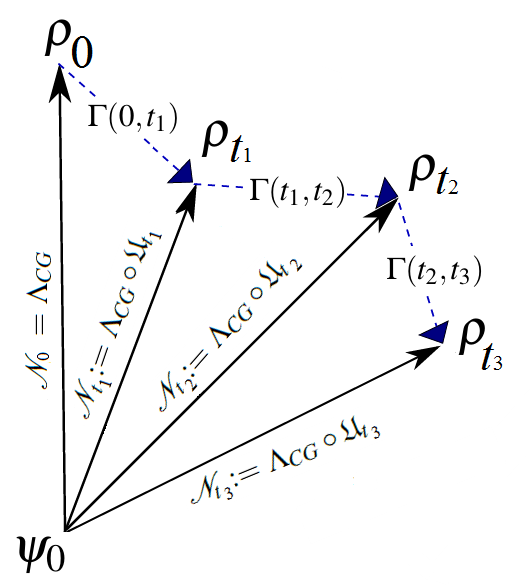
Strict complete positivity can be re-obtained if we demand that the composite map to be CP-divisible Buscemi and Datta (2016). If that is the case, the definition of CP-divisible maps requires for all , with , the effective evolution map for the time interval , completely positive (see Fig. 7). This shows a connection between the theory of coarse grained maps and the theory of non-Markovian maps Buscemi and Datta (2016); Ángel Rivas et al. (2014).
V Consequence: Effective distance increase by
A common property of CPTP linear maps (1), is that the distance between two input states cannot increase. Mathematically, let be a CPTP linear map and and be states in . Then , where the 1-norm is defined as . Physically, this means, for instance, that the discrimination between two unknown quantum states cannot be improved by any further processing of the states Nielsen and Chuang (2000).
The effective map , as discussed in the previous section, is not in general of Kraus form. Can then the distance between two effective states increase? As argued before, no contradiction with quantum mechanics can arise. In fact, it is simple to check that the distance between two effective states is upper-bounded, for all times, by the distance between the underlying initial states. Let and be effective states in with respective evolved states and . Then
| (10) | ||||
| (11) |
The last inequality turns into an equality in the case of a unitary mapping , i.e, for some unitary .
This, however, does not imply that a distance increasing between effective states is not allowed. In fact, it is possible to have an increase in distance between the effective states undergoing the same effective map. Take for example the coarse graining describing the blurred-saturated detector (II.1), the underlying dynamics given by the Hamiltonian (III.1), and select two states and which generate the same effective map IV.2. Figure 8A) shows the distance evolution between the two effective states and . A clear oscillation of the distance is observed. In this example, nevertheless, we have that for all times.
Now, switch on a transversal field, turning the Hamiltonian into , and take initial states , and in a way to have the same effective map. The evolution of the distance between the effective states is shown in Fig. 8B). In this case we see that the distance can go beyond for some specific times.
A)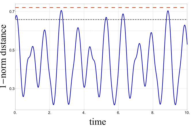
B)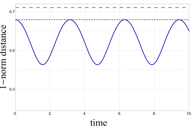
VI Conclusion
When dealing with complex many-body quantum systems, the full description of the system and of its dynamics is prohibitive. Even in principle, it assumes that one has access to all the system’s exponentially (in the number of constituents) many degrees of freedom. A “simple" system composed of qubits, would require in general the measurement of about observables to be fully characterized – even if each measurement is performed in one femtosecond, this would take more than 3000 times the age of the universe to be accomplished. This is only for the state, the characterization of the dynamics is far more complex. Effective descriptions are thus mandatory in order to perceive macroscopic systems.
Pursuing the direction of effective descriptions, here we investigated what types of dynamics may emerge from a full quantum description when one does not have access to, or is not interested in, all the degrees of freedom of a given system. The presented formalism generalizes the theory of open quantum systems, as it works also for closed systems. Here the split between system and environment is substituted by the split between accessible and non-accessible degrees of freedom. The possibility of correlations between these two types of degrees of freedom may generate effective dynamics that are not of Kraus form – without violating any principle of quantum mechanics. This, in turn, allowed for the distance between two effective states to increase under the action of a fixed effective map – in contrast to what is achievable in the underlying quantum description.
Other aspects of this effective dynamics can be further explored. Most notably, the fact that the "Kraus operators" may depend on the state the map is acting on. This suggests a possible way to explain how non-linear dynamics may emerge from the quantum linear description: if one looks at the system only at time intervals for which the term quantifying correlations between accessible and non-accessible degrees of freedom, in Eq. (9), vanishes, i.e., for a coarse grained time Bernardes et al. (2017), then the non-linearity of the first term may become apparent. This (possible) non-linearity, together with the distance increase between effective states undergoing the same effective map may be the key to explain how chaotic systems arise from the underlying quantum mechanical description.
Lastly, we hope that the formalism here presented can shed some light on the quantum-to-classical transition: the higher the "zoom out" (stronger coarse graining, in the sense of larger difference between and ), the more simplified becomes the description of the system and its dynamics, with quantum features fading away. We believe that these ideas can be of interest for areas as quantum thermodynamics – which tries to explain the thermalization of closed quantum systems Eisert et al. (2015); Faist (2016) –, and even to address the measurement problem in quantum mechanics Brukner (2015).
Acknowledgements.
Special thanks goes to Fred Brito, for countless discussions, and careful reading of the manuscript. We also thank R. C. Drumond, D. Jonathan, and R. L. de Matos Filho for stimulating discussions. This work is supported by the Brazilian funding agencies CNPq and CAPES, and it is part of the Brazilian National Institute for Quantum Information.References
- Callen (1985) H. B. Callen, Thermodynamics and an Introduction to Thermostatistics, 2nd ed. (Wiley, 1985).
- Zwanzig (1961) R. Zwanzig, Phys. Rev. 124, 983 (1961).
- Mori (1965) H. Mori, Progress of Theoretical Physics 33, 423 (1965).
- Castiglione et al. (2008) P. Castiglione, M. Falcioni, A. Lesne, and A. Vulpiani, Chaos and Coarse Grainings in Statistical Mechanics (Cambridge University Press, 2008).
- Gell-Mann and Hartle (2014) M. Gell-Mann and J. B. Hartle, Phys. Rev. A 89, 052125 (2014).
- Grabert (1982) H. Grabert, Projection Operator Techniques in Nonequilibrium Statistical Mechanics (Springer Verlag, 1982).
- Kadanoff (1966) L. P. Kadanoff, Physics 2, 263 (1966).
- Wilson (1975) K. G. Wilson, Rev. Mod. Phys. 47, 773 (1975).
- Nielsen and Chuang (2000) M. A. Nielsen and I. L. Chuang, Quantum Computation and Quantum Information (Cambridge University Press, 2000).
- Watrous (2006) J. Watrous, “Theory of quantum information. lecture notes.” (2006), available on-line at https://cs.uwaterloo.ca/watrous/LectureNotes.html.
- Wilde (2017) M. M. Wilde, Quantum Information Theory (Cambridge University Press, 2017).
- Wolf (2012) M. M. Wolf, “Quantum channels & operations,” (2012), available at https://www-m5.ma.tum.de/foswiki/pub/M5/Allgemeines/MichaelWolf/.
- Horodecki et al. (2009) R. Horodecki, P. Horodecki, M. Horodecki, and K. Horodecki, Rev. Mod. Phys. 81, 865 (2009).
- Perez-Garcia et al. (2007) D. Perez-Garcia, F. Verstraete, M. Wolf, and J. Cirac, Quantum Inf. Comput. 7, 401 (2007).
- Orús (2014) R. Orús, Annals of Physics 349, 117 (2014).
- Breuer and Petruccione (2002) H. P. Breuer and F. Petruccione, The Theory of Open Quantum Systems (Oxford University Press, 2002).
- Carteret et al. (2008) H. A. Carteret, D. R. Terno, and K. Zyczkowski, Phys. Rev. A 77, 042113 (2008).
- Štelmachovič and Bužek (2001) P. Štelmachovič and V. Bužek, Phys. Rev. A 64, 062106 (2001).
- Ángel Rivas et al. (2014) Ángel Rivas, S. F. Huelga, and M. B. Plenio, Reports on Progress in Physics 77, 094001 (2014).
- Eisert et al. (2015) J. Eisert, M. Friesdorf, and C. Gogolin, Nat. Phys. 11, 124 (2015).
- Faist (2016) P. Faist, Quantum Coarse-Graining: An Information-Theoretic Approach to Thermodynamics, Ph.D. thesis, ETH Zurich (2016), eprint: arXiv:1607.03104.
- Kofler and Brukner (2007) J. Kofler and C. Brukner, Phys. Rev. Lett. 99, 180403 (2007).
- Kofler and Brukner (2008) J. Kofler and C. Brukner, Phys. Rev. Lett. 101, 090403 (2008).
- Saideh et al. (2016) I. Saideh, S. Felicetti, T. Coudreau, P. Milman, and A. Keller, Phys. Rev. A 94, 032312 (2016).
- herson et al. (2010) J. F. herson, C. Weitenberg, M. Endres, M. Cheneau, I. Bloch, and S. Kuhr, Nature 467, 68 (2010).
- Fukuhara et al. (2015) T. Fukuhara, S. Hild, J. Zeiher, P. Schauß, I. Bloch, M. Endres, and C. Gross, Phys. Rev. Lett. 115, 035302 (2015).
- Preiss et al. (2015) P. M. Preiss, R. Ma, M. E. Tai, A. Lukin, M. Rispoli, P. Zupancic, Y. Lahini, R. Islam, and M. Greiner, Science 347, 1229 (2015), http://science.sciencemag.org/content/347/6227/1229.full.pdf .
- Kuhr (2016) S. Kuhr, National Science Review 3, 170 (2016).
- Buscemi and Datta (2016) F. Buscemi and N. Datta, Phys. Rev. A 93, 012101 (2016).
- Bernardes et al. (2017) N. K. Bernardes, A. R. R. Carvalho, C. H. Monken, and M. F. Santos, Phys. Rev. A 95, 032117 (2017).
- Brukner (2015) C. Brukner, in Quantum [Un]Speakables II: 50 Years of Bell’s Theorem (2015).