Reversal of thermoelectric current in tubular nanowires

Abstract

We calculate the charge current generated by a temperature bias between the two ends of a tubular nanowire. We show that in the presence of a transversal magnetic field the current can change sign, i.e., electrons can either flow from the hot to the cold reservoir, or in the opposite direction, when the temperature bias increases. This behavior occurs when the magnetic field is sufficiently strong, such that Landau and snaking states are created, and the energy dispersion is nonmonotonic with respect to the longitudinal wave vector. The sign reversal can survive in the presence of impurities. We predict this result for core/shell nanowires, for uniform nanowires with surface states due to the Fermi level pinning, and for topological insulator nanowires.

A temperature gradient across a conducing material induces an energy gradient, which in turn results in particle transport. In an open circuit, where no net current flows, a voltage is then generated when two ends of a sample are maintained at different temperatures — this is the Seebeck effect and the linear voltage response is known as thermopower. The hotter particles have larger average kinetic energy, and the net particle flow is therefore generally from the hot to the cold side. The thermopower and thermoelectric current can be positive or negative, depending on the type of charge carriers, i.e., electrons or holes.

In comparison to this macroscopic case, the thermopower at the nanoscale has special characteristics. For example, if the energy separation between the quantum states of the system is larger than the thermal energy the thermopower may alternate between positive and negative values, depending on the position of the Fermi level relatively to a resonant energy, which can be controlled with a gate voltage. These oscillations were predicted a long time ago Beenakker and Staring (1992), and subsequently experimentally observed in quantum dots Staring et al. (1993); Dzurak et al. (1993); Svensson et al. (2012), and in molecules Reddy et al. (2007). A sign change in the thermopower can also be obtained by increasing the temperature gradient and thus the population of the resonant level Svensson et al. (2013); Sierra and Sánchez (2014); Stanciu et al. (2015); Zimbovskaya (2015). In these examples the charge carriers are electrons and the sign change of the thermopower means that they travel from the cold side to the hot side, which may appear counterintuitive. Other nonlinear effects can occur if the characteristic relaxation length of electrons and or phonons exceeds the sample size Sánchez and López (2016), because the energy of electrons and/or phonons is no longer controlled by the temperature of the bath, but by the generated electric bias, including Coulomb interactions Torfason et al. (2013); Sierra et al. (2016).

Observing such negative thermopower at the nanoscale is difficult for at least two reasons: the currents tend to be small and it is hard to maintain a constant temperature difference across such short distances. Here we argue that a generic class of tubular nanowires, to be defined in more detail below, are ideal systems for both realizing and observing negative thermopower. Semiconductor nanowires are versatile systems with complex phenomenology attractive for nanoelectronics. In particular the thermoelectric current increases due to the lateral confinement compared to the values in the bulk material Hicks and Dresselhaus (1993). At the same time the thermal conductivity can be strongly suppressed in nanowires with a diameter below the phonon mean free path Boukai et al. (2008); Zhou et al. (2011). These effects together lead to an increased thermoelectric conversion efficiency in the quasi-one-dimensional geometry.

In the tubular nanowires we are interested in, the conduction takes place only in a narrow shell at the surface, and not through the bulk. This is realized both in so-called core/shell nanowires (CSNs) and topological insulator nanowires (TINs). In CSNs this is a consequence of the structure, the wires being radial heterojunctions of two different materials, a core and a shell. When the shell is a conductor and the core is an insulator, because of the narrow diameter and thickness, typically 50-100 nm and 5-10 nm, respectively, quantum interference effects are present, which have been observed as Aharonov-Bohm magnetoconductance oscillations in longitudinal Gül et al. (2014) and transversal Heedt et al. (2016) magnetic fields, and explained with ballistic transport calculations Rosdahl et al. (2014, 2015); Manolescu et al. (2016). A tubular conductor can also be achieved with nanowires based on a single material, but with surface states radially bound due to the pinning of the Fermi energy Heedt et al. (2016). In the case of TINs, the bulk material is an insulator, but with a topologically nontrivial band structure, that requires a robust metallic state at the surface Hasan and Moore (2011); Bardarson and Moore (2013). Magnetoresistance oscillations, both in longitudinal and transversal fields, were recently reported for TINs made of BiTeSe  Bäßler et al. (2015); Peng et al. (2010); Xiu et al. (2011); Dufouleur et al. (2013); Cho et al. (2015); Jauregui et al. (2016); Dufouleur et al. (2017).

In this paper, then, we consider electrons constrained to move on a cylindrical surface, in the presence of a uniform magnetic field transversal to the axis of the cylinder, and a longitudinal temperature bias. We demonstrate that in these systems a sign reversal of the thermoelectric current is obtained when varying the magnetic field or the temperature bias. Contrary to the cases of molecules and quantum dots, where the sign change of the current is a result of resonant states, in these tubular nanowires the effect is a consequence of a nonmonotonic energy dispersion of electrons vs. momentum. We further show that the sign reversal survives in the presence of a moderate concentration of impurities.

The predicted sign reversal of the thermoelectric current should be detectable in the above mentioned realizations of tubular conductors, but the magnitude of the anomalous current will depend on the specific system parameters. Considering tubular nanowires of 30 nm radius, infinite length, and magnetic fields of 2-4 T, we estimate the magnitude of the anomalous (negative) thermoelectric current as tens of nA. Thermoelectric transport in CSNs has been already studied in a couple of experimental papers. One recent work was the characterization of GaAs/InAs nanowires by thermovoltage measurements in those situations when electrical conductance does not provide information Gluschke et al. (2015). Another study demonstrated enhanced thermoelectric properties in Bi/Te CSNs via strain effects Kim et al. (2017).

Electrons constrained to a cylindrical surface, in the presence of a uniform magnetic field transversal to the axis of the cylinder, have two types of states: $i$) cyclotron orbits at the top and bottom of the cylinder, in the direction of the field, where the radial component of the field is nearly constant, and $ii$) snaking trajectories along the lateral lines where the radial component vanishes and flips orientation, such that the Lorentz force always bends the electron trajectory towards the line Tserkovnyak and Halperin (2006); Ferrari et al. (2009); Manolescu et al. (2013); Chang and Ortix (2017); an illustration is provided in Fig. 1. Such snaking states were studied earlier in the 90’s in a planar electron gas in a perpendicular magnetic field with alternating sign Müller (1992); Ibrahim and Peeters (1995); Zwerschke et al. (1999) and found responsible for strong positive magnetoresistance in the presence of ferromagnetic microstrips Ye et al. (1995); Manolescu and Gerhardts (1997). For our above-mentioned tubular nanowire the snaking states become ground states at nonzero wave vector, imposing a nonmonotonic energy dispersion.

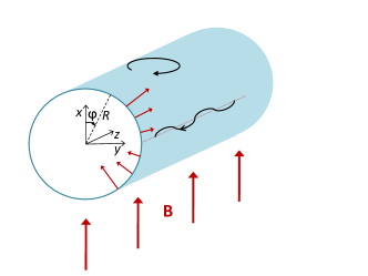
Figure 1: A hollow cylindrical nanowire (light blue) in a uniform transverse magnetic field (thick red arrows). On the top and bottom regions of the cylinder, electrons perform closed cyclotronic loops, whereas on the lateral sides longitudinal snaking orbits are formed along the lines where the radial projection of the magnetic field (thin red arrows) is zero.

To focus, we concentrate our detailed discussion on the case of CSNs; later we will demonstrate that the effects we find are universal and qualitatively the same results are obtained for TINs. We choose the coordinate system such that magnetic field is along the $x$ axis, ${\bf B}=(B,0,0)$, the vector potential being ${\bf A}=(0,0,By)=(0,0,BR\sin\varphi)$. In this case the Hamiltonian can be written as

$$H=\frac{-\hbar^{2}}{2m_{\mathrm{eff}}}\!\left[\frac{\partial^{2}}{R^{2}\partial^{2}\varphi}+(\partial_{z}+\frac{ieBR}{\hbar}\sin\varphi)^{2}\right]\!-\frac{g_{\mathrm{eff}}\mu_{\mathrm{B}}}{2}B\sigma.$$ (1)

In this example we consider material parameters for GaAs, i.e., effective mass $m_{\mathrm{eff}}=0.066$ and $g$-factor $g_{\mathrm{eff}}=-0.44$, $\mu_{\mathrm{B}}$being the Bohr magneton and $\sigma=\pm 1$ the spin label. For $B=0$ the angular part of the Hamiltonian has eigenfunctions $e^{i\varphi n}/\sqrt{2\pi}$, $n\in\mathbb{Z}$, and the single electron energies are ordinary parabolas vs. the wave vector $k$ which is defined by the longitudinal wave functions $e^{ikz}$. These eigenfunctions define a basis set, $|nk\sigma\rangle$, which we use for $B\neq 0$ to diagonalize numerically (1). The convergence is reached with $|n|\leq 50$.

The energy spectra for magnetic fields $B=2.0$ T and $B=4.0$ T are shown in Fig. 3. Since the energy of the cyclotron states increases with $B$, at sufficiently strong fields the low energy bands have a nonmonotonic dispersion, with one maximum around $k=0$ and two lateral symmetric minima. The central maximum corresponds to cyclotron orbits (precursors of Landau levels), and the lateral minima indicate the onset of snaking orbits.

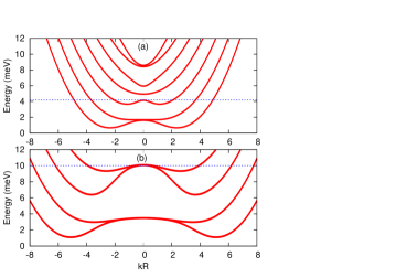
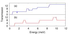
Figure 2: Energy spectra for a cylinder of infinite length and radius $R=30$ nm in a transversal magnetic field $B=2$ T (a) and $B=4$ T (b). The horizontal dotted lines indicate the chemical potential $\mu=4.2$ meV and $\mu=10$ meV, respectively.

Figure 3: Transmission function $T(E)$ for $B=2$ T (a) and $B=4$ T (b). The results are derived with the energy spectra shown in Fig. 3, the circles indicating the location of the chemical potentials. The nonmonotonic behavior of the transmission function is clearly seen.

At any energy each dispersion curve yields a number of propagating modes. The usual situation is with one right moving mode, i.e., with $k>0$, for a given energy. But for energies lying between the central maxima and lateral minima there are two right movers, and accounting for spin results in four in total. Because of the very small $g$-factor the spin splitting is not visible in the figure. When the energy slightly increases above the local maximum, one spin pair of propagation modes is excluded. Hence, the transmission, which in this case is simply the number of propagating modes times $e^{2}/h$, drops two units. The behavior of the transmission function $T(E)$ is seen in Fig. 3, increasing, but also decreasing, in steps as a function of energy, as one would expect from opening and closing modes, respectively. This behavior will lead to the sign reversal of the thermoelectric current.

Such a nonmonotonic behavior of the transmission function is also known for quantum wires with Rashba spin-orbit coupling in a longitudinal magnetic field Nesteroff et al. (2004); Serra et al. (2005). However, the energy scales related to such nonmonotonic transmission are very small and can only be observed in high quality cleaved edge overgrowth samples Quay et al. (2010) at temperatures $\approx 0.3$ K. Very recently a similar effect has been observed in InAs nanowires with a stronger Rashba coupling Heedt et al. (2017). In contrast, in the present case without spin-orbit coupling, the energy scales are much bigger, $T(E)$ is not smeared out by temperature, and leads to a sign reversal of the thermoelectric current.

The charge current through the nanowire, driven by a temperature gradient, can be calculated using the Landauer formula

$$I_{\rm c}=\frac{e}{h}\int T(E)\left[f_{\rm R}(E)-f_{\rm L}(E)\right]dE,$$ (2)

where $f_{\rm L/R}(E)$ are the Fermi functions for the left/right reservoir with chemical potentials $\mu_{\rm L/R}$ and temperatures $T_{\rm L/R}$. We consider a temperature bias, $T_{\rm R}>T_{\rm L}$, beyond linear response, and no potential bias, such that the difference of the Fermi functions changes sign at $E=\mu_{\rm L}=\mu_{\rm R}$. Coulomb interactions are neglected, which is a good approximation for widely open wires. If the transmission function $T(E)$ increases with energy over the integration interval the thermoelectric current is positive, i.e., the electrons flow from the hot contact to the cold one. This is the normal situation. An anomalous negative current instead occurs if the transmission function decreases with energy, as shown in Fig. 3. The energy integral is calculated numerically using the trapezoidal method. We keep the left reservoir at a fixed temperature, $T_{\rm L}=0.5$ K, i.e., low, but non-zero as in experimental setups. By varying the temperature of the right reservoir we obtain the current as function of $T_{\rm R}$, as shown in Fig. 4, where one can notice that the sign of the current may change both with $T_{\rm R}$ or magnetic field.

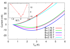
Figure 4: Thermoelectric current as a function of the temperature of the right contact $T_{\rm R}$ for the indicated magnetic field values and $\mu=4.2$ meV. The inset shows the current as a function of magnetic field for a fixed temperature $T_{\rm R}=3$ K marked with a vertical line in the main figure. The left contact is kept at constant temperature $T_{\rm L}=0.5$ K.

The anomalous current can be in the range of tens of nA, i.e., much larger than for quantum dots. The largest value shown in Fig. 4 is about -10 nA for $B=2$ T and $T_{\rm R}=2.5$ K. With a magnetic field of $B=4$ T, yielding the energy spectrum of Fig. 3(b), we could obtain, in the ballistic case, an anomalous current of nearly -60 nA at $T_{\rm R}=8$ K, as shown in Fig. 5.

The appearance of the anomalous current relies on nonmonotonic steps in the transmission function. For clean wires the steps are sharp, but in the presence of impurities the steps will get rounded. The transmission function in the case when impurities are included is obtained using the recursive Green’s function method . Here we simulate transport in a nanowire where the impurities are assumed to be short range,

$$V_{\mathrm{imp}}(z,\varphi)=\sum_{i}W\delta(z-z_{i})\delta(\varphi-\varphi_{i})\ ,$$ (3)

where $W$ is the impurity strength. We consider a fixed impurity configuration, i.e., no ensemble average. To some extent the results depend on the impurity configuration, as also seen in experiments. There the conductance can show complicated, but reproducible behavior for a given nanowire , whereas the conductance for another nanowire will yield conductance whose structure (position of peaks, etc.) will be different Wu et al. (2013), but reproducible as well. The average density of impurities is chosen $n_{\mathrm{imp}}=3.0$ nm^-1 and the disorder strength $W=1.2\hbar^{2}/(2m_{\rm{eff}}R^{2})$. We consider repulsive impurities, $W>0$, since negative values of $W$ lead to a strong suppression of the conductance when electrons get bound at potential minima. The key point is that as long as the transmission function still shows the nonmonotonic steps the anomalous current is obtained. In Fig. 5 we compare the thermoelectric currents for the same magnetic field and chemical potential, in the ballistic case and with a fixed impurity concentration.

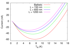
Figure 5: Thermoelectric current calculated with the energy spectra shown in Fig. 3 ($B=4$ T, $\mu=10$ meV) in the ballistic case and for randomly distributed impurities within a scattering region of size $L=150,600,\ {\rm and}\ 1200$ nm.

Indeed, the magnitude of the anomalous current is reduced in the presence of impurities. It further drops for longer wires due to the increased number of scattering events, but it is still sizeable. Instead, the magnitude of the normal current increases with the number of scatterers. This is because the contribution of the transmission bumps decreases and the transition point $I_{\rm c}=0$ shifts to lower and lower temperatures. Of course, if the nanowire is too dirty, such that the conductance becomes a series of transmission resonances due to quantum dotlike states Wu et al. (2013), the anomalous current will not be observable. However, even in that case the transport calculations based on elastic scattering reproduced well the thermopower measurements up to 24 K Wu et al. (2013). This makes us confident that inelastic collisions can also be neglected in our temperature range.

Having considered the CSN case in detail, we now briefly discuss the case of TINs. Such wires in a magnetic field have recently been studied extensively both theoretically Bardarson et al. (2010); Zhang and Vishwanath (2010); Zhang et al. (2012); Ilan et al. (2015); Xypakis and Bardarson (2017) and experimentally Peng et al. (2010); Xiu et al. (2011); Dufouleur et al. (2013); Cho et al. (2015); Jauregui et al. (2016); Dufouleur et al. (2017); Arango et al. (2016). In contrast to the Schrödinger fermions of the CSNs, the surface states of the topological insulator are Dirac fermions, described by the Hamiltonian Bardarson et al. (2010); Zhang and Vishwanath (2010); Bardarson and Moore (2013)

$$H_{\mathrm{TI}}=-i\hbar v_{F}\left[\sigma_{z}\left(\partial_{z}+i\frac{eB}{\hbar}R\sin\varphi\right)+\sigma_{y}\frac{1}{R}\partial_{\varphi}\right],$$ (4)

where $v_{F}$ is the Fermi velocity, and the spinors satisfy antiperiodic boundary conditions $\hat{\psi}(\varphi)=-\hat{\psi}(\varphi+2\pi)$, due to a Berry phase. It is convenient to diagonalize (4) using the same angular basis states as before, but because of the boundary condition $n$ now takes half-integer values. An example of the energy spectrum is shown in Fig. 6(a) where, as in the CSN case, precursors of Landau levels around $k=0$ are seen, both at negative and positive energy, and snaking states are visible at the edges. These states give rise to transmission that decreases with energy, as shown in Fig. 6(b), and consequently to an anomalous thermoelectric current, as before, shown now in Fig. 6(c). The TINs offer some further advances. For example, the surface states are robust to disorder, and the negative gradient in the transmission is also obtained at relatively strong disorder strengths.

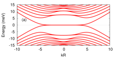
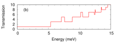
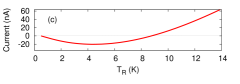
Figure 6: The energy spectrum (a), transmission function (b), and thermoelectric current (c), for a TIN with $v_{F}=10^{5}$ m/s, $R=30$ nm, and $B=4.3$ T.

In conclusion, an unexplored consequence of the coexistence of snaking and Landau states in tubular nanowires in a transverse magnetic field is that the transmission function is nonmonotonic with the energy, which implies that the thermoelectric current can be both positive and negative.  The normal flow of electrons should be from the hot to the cold contact.  Instead, in a magnetic field of a few Tesla and variable temperature of the hot source, here below 10 K, an anomalous flow occurs, from the cold lead to the hot lead, corresponding to tens of nA. This phenomenon can have applications to thermoelectric devices based on nanowires. In particular, the detection of the current reversal can be seen as an indication of the tubular distribution of the conduction electrons, which is crucial for topological insulator nanowires. The presence of snaking states has already been detected both in CSNs Heedt et al. (2016) and in TINs Bäßler et al. (2015), and hence the predicted anomalous current should be within the experimental reach. Identifying the general relationship between the thermocurrent and nonmonotonic transmission function can motivate the study of the anomalous current in other systems.

This work was supported by: RU Fund 815051 TVD, ANCSI Grant PN16420202, MINECO Grant FIS2014-52564, and ERC Starting Grant 679722.

*

Appendix A Supplemental Material: Computational method for core/shell nanowires with impurities

A.1 Green’s function discretization

Our starting point is the partial differential equation for the Green’s function of the tubular nanowire

$$\left(E-\left[-\frac{\hbar^{2}}{2mR^{2}}\partial_{\varphi}^{2}+\frac{1}{2m}\left(\frac{\hbar}{i}\partial_{z}+eBR\sin\varphi\right)^{2}\right]\right)G^{r}(z,z^{\prime},\varphi,\varphi^{\prime};E)=\delta(z-z^{\prime})\delta(\varphi-\varphi^{\prime}).$$ (1)

Next, we write $G^{r}$ as a Fourier series in $(\varphi,\varphi^{\prime})$

$$G^{r}(z,z^{\prime},\varphi,\varphi^{\prime};E)=\frac{1}{2\pi}\sum_{n,n^{\prime}\in\mathbb{Z}}e^{-in\varphi}e^{in^{\prime}\varphi^{\prime}}G^{r}_{n,n^{\prime}}(z,z^{\prime}),$$ (2)

with Fourier components

$$G^{r}_{n,n^{\prime}}(z,z^{\prime})=\frac{1}{2\pi}\int d\varphi d\varphi^{\prime}e^{in\varphi}e^{in^{\prime}\varphi^{\prime}}G^{r}(z,z^{\prime},\varphi,\varphi^{\prime};E).$$ (3)

Note that we have dropped the $E$ from $G^{r}_{n,n^{\prime}}$ for sake of brevity. Inserting Eq. (2) into Eq. (1), multiplying with $e^{-im\varphi}e^{im^{\prime}\varphi^{\prime}}/2\pi$ and integrating over $(\varphi,\varphi^{\prime})$ results in

$$\frac{\hbar^{2}}{2mR^{2}}\sum_{n\in\mathbb{Z}}\left(\left(\mathcal{E}-(n^{2}-R^{2}\partial_{z}^{2})\right)\delta_{m,n}+2i(R\partial_{z})\frac{R^{2}}{\ell_{c}^{2}}[\sin\varphi]_{m,n}-\frac{R^{4}}{\ell_{c}^{4}}[\sin^{2}\varphi]_{m,n}\right)G^{r}_{n,m^{\prime}}(z,z^{\prime})=\delta(z-z^{\prime})\delta_{m,m^{\prime}}$$ (4)

Here we introduced $\mathcal{E}$ which measures energy in units of $\frac{\hbar^{2}}{2mR^{2}}$ and

$$[f(\varphi)]_{m,n}=\frac{1}{2\pi}\int d\varphi e^{-im\varphi}e^{in\varphi}f(\varphi).$$ (5)

Equation (4) can be written more compactly on matrix form

$$\frac{\hbar^{2}}{2mR^{2}}\left[(\mathcal{E}+R^{2}\partial_{z}^{2})\mathbb{I}-\mathrm{diag}(n^{2})-2i(R\partial_{z})\frac{R^{2}}{\ell_{c}^{2}}[\sin\varphi]-\frac{R^{4}}{\ell_{c}^{4}}[\sin^{2}\varphi])\right]G^{r}(z,z^{\prime})=\delta(z-z^{\prime})\mathbb{I}$$ (6)

Here all matrices are assumed to be of dimension $(2M_{\mathrm{max}}+1)$, i.e. a cut-off has be introduced here such that $n\in[-M_{\mathrm{max}},M_{\mathrm{max}}]$. This is now a equivalent to a one dimensional problem with an internal degree of freedom and one can proceed with standard finite difference implementation where the continuous variable $z$ is discretized. Introducing a lattice parameter $a$ and the notation $z_{i+1}=z_{i}+a$, the finite difference version becomes

$$\left(E\mathbb{I}-\frac{\hbar^{2}}{2mR^{2}}\left[\mathrm{diag}(n^{2})+\frac{R^{4}}{\ell_{c}^{4}}[\sin^{2}\varphi]+\frac{2R^{2}}{a^{2}}\mathbb{I}\right]\right)G^{r}(z_{i},z_{j})$$

$$+\frac{\hbar^{2}}{2mR^{2}}\left[-\frac{R^{2}}{a^{2}}\mathbb{I}-i\frac{R}{a}\frac{R^{2}}{\ell_{c}^{2}}[\sin\varphi]\right]G^{r}(z_{i+1},z_{j})+\frac{\hbar^{2}}{2mR^{2}}\left[-\frac{R^{2}}{a^{2}}\mathbb{I}+i\frac{R}{a}\frac{R^{2}}{\ell_{c}^{2}}[\sin\varphi]\right]G^{r}(z_{i-1},z_{j})=\delta_{i,j}\mathbb{I},$$ (7)

or in a more compact form

$$\left(E\mathbb{I}-H_{\mathrm{sl}}\right)G^{r}(z_{i},z_{j})+V_{\mathrm{sl}}G^{r}(z_{i+1},z_{j})+V_{\mathrm{sl}}^{\dagger}G^{r}(z_{i-1},z_{j})=\delta_{i,j}\mathbb{I},$$ (8)

where we have defined the slice Hamiltonian

$$H_{\mathrm{sl}} = \frac{\hbar^{2}}{2mR^{2}}\left(\left(\mathrm{diag}(n^{2})+\frac{2R^{2}}{a^{2}}\mathbb{I}\right)+\frac{R^{4}}{\ell_{c}^{4}}[\sin^{2}]\right),$$ (9)

and the slice coupling Hamiltonian

$$V_{\mathrm{sl}} = \frac{\hbar^{2}}{2mR^{2}}\left(-\frac{R^{2}}{a^{2}}\mathbb{I}+2i\frac{R^{2}}{\ell_{c}^{2}}\frac{R}{2a}[\sin\varphi]\right).$$ (10)

Note that $V_{\mathrm{sl}}$ is not hermitian, and does not have to be, since the full Hamiltonian of the entire system contains both $V_{\mathrm{sl}}$ and $V_{\mathrm{sl}}^{\dagger}$. This is well known in the case of a discretized 2D slab in a non-zero transverse magnetic field where $V_{\mathrm{sl}}$ becomes complex via the Peierls substitution Peierls (1933); Ferry and Goodnick (1997).

Since Eq. (8) is of the standard hopping or tight-binding type, one can follow standard methods outlined in e.g. Ref. Ferry and Goodnick, 1997. Note that in the absence of magnetic field all the matrices become diagonal and the coupling will simply be determined by the standard tight-binding parameter $t=\frac{\hbar^{2}}{2ma^{2}}$. Physically this means that the eigenmodes $\langle\varphi|n\rangle$ decouple, the different modes are independent and shifted in energy depending on the transverse quantization $\frac{\hbar^{2}}{2mR^{2}}n^{2}$.

To describe a wire in the quasi-ballistic regime the discrete values $z_{i}$ are separated into left, central, and right part, see Fig. A1. The impurities only occur in the central part, where the short range impurity Hamiltonian (Eq. (3) in the manuscript) is discretized leading to a new Hamiltonian for slice $i$

$$H_{i}=H_{\mathrm{sl}}+V_{\mathrm{imp},i}.$$ (11)

In the left and right parts of the system all the slice Hamiltonians, and slice couplings, are the same, $H_{\mathrm{sl}}$ and $V_{\mathrm{sl}}$ respectively, the self-energies can be calculated using a very fast, versatile algorithm Sancho et al. (1985). Note that the self-energies only enter the slice Hamiltonians for slice $i=1$ ($\Sigma_{L}$) and $i=N$ ($\Sigma_{R}$). Once the self-energies are found, as a function of energy the Green’s function in the central region can be found using the recursive Green’s function method Ferry and Goodnick (1997). From the recursive algorithm one obtains $G^{r}_{z_{1},z_{N}}(E)$, the part of the Green’s function that describes the connection of the first slice (1) and the last slice ($N$), see bottom of Fig. A1. Finally, after the Green’s function is obtained the transmission function can found using the Fisher-Lee relation Fisher and Lee (1981).

$$T(E)=\mathrm{tr}\{\hat{\Gamma}_{L}(E)G^{r}(z_{1},z_{N})(E)\hat{\Gamma}_{R}(E)(G^{r}(z_{1},z_{N})(E))^{\dagger}\},$$ (12)

where $\hat{\Gamma}_{\alpha}(E)=-i(\hat{\Sigma}_{\alpha}(E)-(\hat{\Sigma}_{\alpha}(E))^{\dagger})$ for $\alpha=L,R$.

\psfrag{Rth}{ $R\theta$}\psfrag{zz}{$z$}\psfrag{SL}{$\Sigma_{L}$}\psfrag{SR}{$\Sigma_{R}$}\psfrag{H0}{$H_{\mathrm{sl}}$}\psfrag{VV}{$V_{\mathrm{sl}}$}\psfrag{VD}{$V_{\mathrm{sl}}^{\dagger}$}\psfrag{Hi}{\!\!\!\! $H_{i}$}\psfrag{dots}{$\dots$}\psfrag{ii}{$z_{i}$}\psfrag{i1}{\!\!\!$z_{1}$}\psfrag{iN}{\!\!\!$z_{N}$}\includegraphics[width=303.53267pt]{figures/sys1.eps}

Figure A1: The tubular nanowire represented as a rolled out rectangular sheet. The top figures shows the impurities distributed randomly in the central part. The middle figure shows the impurities after they are shifted to a discrete value $z_{i}$, depending on their initial position. The bottom figures shows a one-dimensional tight-binding model with slice matrices $H_{i}$ in the central part and coupling matrices $V_{\mathrm{sl}}$. The left (right) infinite parts gives rise to self-energies $\Sigma_{L}$ ($\Sigma_{R}$) that inter $H_{1}$ ($H_{N}$).

A.2 Choice of lattice parameter $a$

In zero magnetic field the lattice version of the Green’s function, Eq. (7) is diagonal in the angular basis, so the system consists of independent one-dimensional modes. The dispersion of a nearest neighbor tight binding system with coupling $t=\frac{\hbar^{2}}{2ma}$ is

$$\varepsilon(k) = 2t(1-\cos(ka)).$$ (13)

To use the discretization as an approximation to the continuum version, the value of $a$ needs to be small enough such that Eq. (13) is close enough to the correct parabolic dispersion up to some relevant maximum value of $k$. A natural choice for the maximum value is $k_{M}=\tfrac{M}{R}$ which corresponds to having parabolic dispersion up to transverse state $M$ with energy $\tfrac{\hbar^{2}}{2mR^{2}}M^{2}$. To quantify the relative deviation of the cosine dispersion from the parabolic one, we use

$$\left.\frac{\frac{\hbar^{2}k^{2}}{2m}-\varepsilon(k)}{\frac{\hbar^{2}k^{2}}{2m}}\right|_{k=\frac{M}{R}}=1-\frac{1}{M^{2}}\frac{R^{2}}{a^{2}}2\left(1-\cos\left(M\frac{a}{R}\right)\right)<\eta,$$ (14)

where $\eta$ is the required relative accuracy. Now, writing $a=s\tfrac{R}{M}$, where $s$ is dimensionless quantity, we have

$$1-\frac{2}{s^{2}}\left(1-\cos\left(s\right)\right)<\eta.$$ (15)

For a given value of $\eta$, e.g. $\eta=0.01$, one obtains that $s<0.35$ will give a $1\%$ relative accuracy.

When a non-zero magnetic field is considered, this procedure does not strictly hold. However, when a confined system with typical size $R$ is subjected to an external magnetic field the relevant length scale becomes the magnetic length $\ell_{c}$, for large enough magnetic fields. To reflect this cross-over of length scales we use

$$a = 0.35\frac{R}{M}\left(1+\frac{R^{4}}{\ell_{c}^{4}}\right)^{-1/4}.$$ (16)

As a final check we do check that numerical results (energy spectrum and transmission function) does not change significantly for smaller values of $a$.

References

- Beenakker and Staring (1992) C. W. J. Beenakker and A. A. M. Staring, Phys. Rev. B 46, 9667 (1992).
- Staring et al. (1993) A. A. M. Staring, L. W. Molenkamp, B. W. Alphenaar, H. van Houten, O. J. A. Buyk, M. A. A. Mabesoone, C. W. J. Beenakker, and C. T. Foxon, Europhys. Lett. 22, 57 (1993).
- Dzurak et al. (1993) A. Dzurak, C. Smith, M. Pepper, D. Ritchie, J. Frost, G. Jones, and D. Hasko, Solid State Commun. 87, 1145 (1993).
- Svensson et al. (2012) S. F. Svensson, A. I. Persson, E. A. Hoffmann, N. Nakpathomkun, H. A. Nilsson, H. Q. Xu, L. Samuelson, and H. Linke, New Journal of Physics 14, 033041 (2012).
- Reddy et al. (2007) P. Reddy, S.-Y. Jang, R. A. Segalman, and A. Majumdar, Science 315, 1568 (2007).
- Svensson et al. (2013) S. F. Svensson, E. A. Hoffmann, N. Nakpathomkun, P. Wu, H. Q. Xu, H. A. Nilsson, D. Sánchez, V. Kashcheyevs, and H. Linke, New Journal of Physics 15, 105011 (2013).
- Sierra and Sánchez (2014) M. A. Sierra and D. Sánchez, Phys. Rev. B 90, 115313 (2014).
- Stanciu et al. (2015) A. E. Stanciu, G. A. Nemnes, and A. Manolescu, Romanian J. Phys. 60, 716 (2015).
- Zimbovskaya (2015) N. A. Zimbovskaya, J. Chem. Phys. 142, 244310 (2015).
- Sánchez and López (2016) D. Sánchez and R. López, Comptes Rendus Physique 17, 1060 (2016).
- Torfason et al. (2013) K. Torfason, A. Manolescu, S. I. Erlingsson, and V. Gudmundsson, Physica E 53, 178 (2013).
- Sierra et al. (2016) M. A. Sierra, M. Saiz-Bretín, F. Domínguez-Adame, and D. Sánchez, Phys. Rev. B 93, 235452 (2016).
- Hicks and Dresselhaus (1993) L. D. Hicks and M. S. Dresselhaus, Phys. Rev. B 47, 16631 (1993).
- Boukai et al. (2008) A. I. Boukai, Y. Bunimovich, J. Tahir-Kheli, J.-K. Yu, W. A. Goddard III, and J. R. Heath, Nature 451, 168 (2008).
- Zhou et al. (2011) F. Zhou, A. L. Moore, J. Bolinsson, A. Persson, L. Fröberg, M. T. Pettes, H. Kong, L. Rabenberg, P. Caroff, D. A. Stewart, N. Mingo, K. A. Dick, L. Samuelson, H. Linke, and L. Shi, Phys. Rev. B 83, 205416 (2011).
- Gül et al. (2014) O. Gül, N. Demarina, C. Blömers, T. Rieger, H. Lüth, M. I. Lepsa, D. Grützmacher, and T. Schäpers, Phys. Rev. B 89, 045417 (2014).
- Heedt et al. (2016) S. Heedt, A. Manolescu, G. A. Nemnes, W. Prost, J. Schubert, D. Grützmacher, and T. Schäpers, Nano Lett. 16, 4569 (2016).
- Rosdahl et al. (2014) T. O. Rosdahl, A. Manolescu, and V. Gudmundsson, Phys. Rev. B 90, 035421 (2014).
- Rosdahl et al. (2015) T. O. Rosdahl, A. Manolescu, and V. Gudmundsson, Nano Lett. 15, 254 (2015).
- Manolescu et al. (2016) A. Manolescu, G. A. Nemnes, A. Sitek, T. O. Rosdahl, S. I. Erlingsson, and V. Gudmundsson, Phys. Rev. B 93, 205445 (2016).
- Hasan and Moore (2011) M. Z. Hasan and J. E. Moore, Annu. Rev. Cond. Matt. Phys. 2, 55 (2011).
- Bardarson and Moore (2013) J. H. Bardarson and J. E. Moore, Reports Prog. Phys. 76, 056501 (2013).
- Bäßler et al. (2015) S. Bäßler, B. Hamdou, P. Sergelius, A.-K. Michel, R. Zierold, H. Reith, J. Gooth, and K. Nielsch, Appl. Phys. Lett. 107, 181602 (2015).
- Peng et al. (2010) H. Peng, K. Lai, D. Kong, S. Meister, Y. Chen, X.-L. Qi, S. C. Zhang, Z.-X. Shen, and Y. Cui, Nature Mater. 9, 225 (2010).
- Xiu et al. (2011) F. Xiu, L. He, Y. Wang, L. Cheng, L.-T. Chang, M. Lang, G. Huang, X. Kou, Y. Zhou, X. Jiang, Z. Chen, J. Zou, A. Shailos, and K. L. Wang, Nature Nanotech. 6, 216 (2011).
- Dufouleur et al. (2013) J. Dufouleur, L. Veyrat, A. Teichgräber, S. Neuhaus, C. Nowka, S. Hampel, J. Cayssol, J. Schumann, B. Eichler, O. G. Schmidt, B. Büchner, and R. Giraud, Phys. Rev. Lett. 110, 186806 (2013).
- Cho et al. (2015) S. Cho, B. Dellabetta, R. Zhong, J. Schneeloch, T. Liu, G. Gu, M. J. Gilbert, and N. Mason, Nature Commun. 6, 7634 (2015).
- Jauregui et al. (2016) L. A. Jauregui, M. T. Pettes, L. P. Rokhinson, L. Shi, and Y. P. Chen, Nature Nanotech. 11, 345 (2016).
- Dufouleur et al. (2017) J. Dufouleur, L. Veyrat, B. Dassonneville, E. Xypakis, J. H. Bardarson, C. Nowka, S. Hampel, J. Schumann, B. Eichler, O. G. Schmidt, B. Büchner, and R. Giraud, Scientific Reports 7, 45276 (2017).
- Gluschke et al. (2015) J. G. Gluschke, M. Leijnse, B. Ganjipour, K. A. Dick, H. Linke, and C. Thelander, ACS Nano 9, 7033 (2015).
- Kim et al. (2017) J. Kim, G. Kim, J.-H. Bahk, J.-S. Noh, and W. Lee, Nano Energy 32, 520 (2017).
- Tserkovnyak and Halperin (2006) Y. Tserkovnyak and B. I. Halperin, Phys. Rev. B 74, 245327 (2006).
- Ferrari et al. (2009) G. Ferrari, G. Goldoni, A. Bertoni, G. Cuoghi, and E. Molinari, Nano Lett. 9, 1631 (2009).
- Manolescu et al. (2013) A. Manolescu, T. Rosdahl, S. Erlingsson, L. Serra, and V. Gudmundsson, Eur. Phys. J. B 86, 445 (2013).
- Chang and Ortix (2017) C.-H. Chang and C. Ortix, Int. J. Mod. Phys. B 31, 1630016 (2017).
- Müller (1992) J. E. Müller, Phys. Rev. Lett. 68, 385 (1992).
- Ibrahim and Peeters (1995) I. S. Ibrahim and F. M. Peeters, Phys. Rev. B 52, 17321 (1995).
- Zwerschke et al. (1999) S. D. M. Zwerschke, A. Manolescu, and R. R. Gerhardts, Phys. Rev. B 60, 5536 (1999).
- Ye et al. (1995) P. D. Ye, D. Weiss, R. R. Gerhardts, M. Seeger, K. von Klitzing, K. Eberl, and H. Nickel, Phys. Rev. Lett. 74, 3013 (1995).
- Manolescu and Gerhardts (1997) A. Manolescu and R. R. Gerhardts, Phys. Rev. B 56, 9707 (1997).
- Nesteroff et al. (2004) J. A. Nesteroff, Y. V. Pershin, and V. Privman, Phys. Rev. Lett. 93, 126601 (2004).
- Serra et al. (2005) L. Serra, D. Sánchez, and R. López, Phys. Rev. B 72, 235309 (2005).
- Quay et al. (2010) C. Quay, T. Hughes, J. Sulpizio, L. Pfeiffer, K. Baldwin, K. West, D. Goldhaber-Gordon, and R. de Picciotto, Nature Phys. 6, 336 (2010).
- Heedt et al. (2017) S. Heedt, N. Traverso Ziani, F. Crépin, W. Prost, S. Trellenkamp, J. Schubert, D. Grützmacher, B. Trauzettel, and T. Schäpers, Nature Phys. 13, 563 (2017).
- Note (1) The computational details are described in the Supplemental Material.
- Note (2) Here reproducible means that the measurement can be repeated later on the same nanowire and it will give the same conductance plot.
- Wu et al. (2013) P. M. Wu, J. Gooth, X. Zianni, S. F. Svensson, J. G. Gluschke, K. A. Dick, C. Thelander, K. Nielsch, and H. Linke, Nano Lett. 13, 4080 (2013).
- Bardarson et al. (2010) J. H. Bardarson, P. W. Brouwer, and J. E. Moore, Phys. Rev. Lett. 105, 156803 (2010).
- Zhang and Vishwanath (2010) Y. Zhang and A. Vishwanath, Phys. Rev. Lett. 105, 206601 (2010).
- Zhang et al. (2012) Y.-Y. Zhang, X.-R. Wang, and X. C. Xie, J. Phys. Condens. Matter 24, 015004 (2012).
- Ilan et al. (2015) R. Ilan, F. De Juan, and J. E. Moore, Phys. Rev. Lett. 115, 096802 (2015).
- Xypakis and Bardarson (2017) E. Xypakis and J. H. Bardarson, Phys. Rev. B 95, 035415 (2017).
- Arango et al. (2016) Y. C. Arango, L. Huang, C. Chen, J. Avila, M. C. Asensio, D. Grützmacher, H. Lüth, J. G. Lu, and T. Schäpers, Sci. Rep. 6, 29493 (2016).
- Peierls (1933) R. Peierls, Z. Phys. 80, 763 (1933).
- Ferry and Goodnick (1997) D. K. Ferry and S. M. Goodnick, Transport in Nanostructures, edited by H. Ahmed, M. Pepper, and A. Broers (Cambridge University Press, Cambridge, 1997).
- Sancho et al. (1985) M. L. Sancho, J. L. Sancho, and J. Rubio, J. Phys. F: Metal Physics 15, 851 (1985).
- Fisher and Lee (1981) D. Fisher and P. Lee, Phys. Rev. B 23, 6851 (1981).
*