Quantitative Estimates in Homogenization of Parabolic Systems of Elasticity
in Lipschitz Cylinders
Abstract
This paper is devoted to establish an almost sharp error estimate in -norm for homogenization of parabolic systems of elasticity with initial-Dirichlet conditions in a Lipschitz cylinder.
To achieve the goal, with the parabolic distance function being a weight, we first develop
some new weighted-type inequalities for the smoothing operator
at scale in terms of t-anisotropic Sobolev spaces, and then reduce
all the problems to three kinds of estimate for the homogenized system, in which a weighted-type Caccioppoli’s inequality on time-layer has been found. Throughout the paper,
we do not require any smoothness on coefficients compared to
the arguments investigated by C.Kenig, F. Lin and Z. Shen in [17]. This study
can be considered to be a further development of [10] and [27].
Key words: homogenization; parabolic systems; elasticity; error estimates;
Lipschitz cylinders.
1 Introduction and main results
In recent years, J. Geng and Z. Shen in [9, 10] have made some significant developments in quantitative homogenization of parabolic systems with time-dependent periodic coefficients, such as the uniform , Hölder and interior Lipschitz estimates, as well as a sharp convergence rate. Meanwhile, for parabolic systems only involving spatial-dependent periodic coefficients, a sharp error estimate has also been obtained by Yu. Meshkova and T. Suslina in [19]. However, all the results in previous references were merely established for smooth cylinders. In this paper, we manage to study the nonsmooth case.
We begin by stating the initial-boundary value problems that we will investigate and sketching our main results. Let with be a bounded Lipschitz domain. For satisfying , we define the parabolic cylinder as , and the lateral boundary of as , while the parabolic boundary of is written by .
For given data , and specified in some proper spaces, we consider the following parabolic system of elasticity with a initial-Dirichlet condition:
where is a small parameter, and
(Einstein’s convention for summation is used throughout.)
Let with be real and satisfy two hypotheses.
-
1.
Elasticity: there holds
(1.1) for any and symmetric matrix , where .
-
2.
Periodicity: for and ,
(1.2)
We now state the first result.
Theorem 1.1.
Suppose that satisfies and . Let , and . Then for a family of weak solutions with to , there holds strongly in , as , where satisfies the homogenized system:
in a weak sense, and is an operator with the constant coefficient specified in .
Here means its component with , and its definition may be found in [8, pp.374]. By the same convention, the notation , , and represent the corresponding product spaces, in which the space is a Hilbert space collecting functions with one half of a spatial derivative and one quarter of a time derivative in (see [7, pp.502]), and the definition of is stated in [8, pp.301]. We remark that there is little effort made to distinguish vector-valued functions or function spaces from their real-valued counterparts in the paper.
Up to the first Korn inequality stated in [16, pp.371], the proof of Theorem 1.1 is quite similar to that given for [9, Theorem 3.1] in the case of , and we just outline it in Section 2. Also, on account of [9, Remark 3.2] the homogenized system is still a parabolic system with the constant coefficient satisfying the same elasticity condition . The above result is just a qualitative investigation, and this kind research may trace back to 1970s, which was summarized in the monograph [4, pp.140]. In the paper, we will seek for a sharply quantitative estimate on rate of convergence between and in , and the following theorem gives the main result.
Theorem 1.2.
Suppose that satisfies the conditions and . Given , and , let and be the weak solutions of the initial-Dirichlet problems and , respectively. Then we have
| (1.3) |
where depends only on and .
The symbol denotes a Sobolev space of functions with one spatial derivative and half of a time derivative in , requiring its element to vanish on (see [6, pp.353]). This may be viewed as a compatibility condition between the lateral data and the initial data .
The convergence rate estimate is almost sharp, which may be interpreted as an operator error estimate sometimes. Compared to the recent result obtained in [10, Theorem 1.1], the estimate owns two conspicuous advantages. One is that the result is established for a Lipschitz cylinder, the other is that the estimate is fully based upon the given data, especially permitting a lower regularity assumption on the lateral data . On the other hand, the estimate is quite similar to that developed for elliptic systems with Dirichlet or Neumann boundary conditions in [27, Theorems 1.1,1.2], which seems to be reasonable if we think of the elliptic system as the stable case of the parabolic one. However, handling parabolic systems proved to be much complicated, and we have to establish some new weighted-type estimates with a parabolic distance function being a weight, such as Lemmas and 2.9. Meanwhile, some new techniques designed for the so-called time-layer type estimates have also been developed in Lemmas 3.6 and 4.2. Such the estimates similar to have been intensively studied during the past ten years for elliptic operators, parabolic equations and Stokes systems in periodic homogenization theory, and without attempting to be exhaustive we refer the reader to [1, 2, 3, 4, 5, 10, 11, 12, 13, 14, 17, 19, 21, 23, 24, 25, 27, 28, 29, 30] and references therein for more results. We end this paragraph by mention that the source of the main ideas directly come from the references [10, 27], originally from C. Kenig, F. Lin, Z. Shen and T. Suslina in [17, 21, 25].
So, it is instructive to sketch the main procedures before giving the detailed proof. Inspired from [10, Theorem 2.2], we construct the approximating of as follows
| (1.4) |
where and with , are known as correctors and dual correctors in Subsection 2.3, and they had been well studied in [9, 10]. Here and is the smoothing operators given in Definition 1, as successors of the so-called Steklov smoothing operator originally applied to the homogenization problems by V.V Zhikov and S.E. Pastukhova in [30]. The notation is a cut-off function whose description will be given later. Then, we can find an equation that satisfies (see Lemma 3.1), and this is the starting point of the proof of Theorem 1.2. For ease of statement, it is fine to assume by the linearity of and . Roughly speaking, the proof will be reduced to two steps. The first one is based upon the energy inequality, which shows
| (1.5) |
The second one relies on duality methods, by which we may establish
| (1.6) |
At a glimpse, the methods look similar to the aforementioned ones as in [10]. However, the calculations related to nonsmooth cylinders turn to be much involved. So, some related tricks are necessary to be explained. Before proceeding further, it is better to introduce some geometric notation to simplify the later statements, and they will be shown in Figures • ‣ 1 and • ‣ 1 to make them be apprehended at a glance.
-
•
denotes the level set of .
-
•
is the diameter of , and denotes the the internal diameter, where is an open ball in with center and radius , and we call the layer constant.
-
•
is known as a parabolic cube with the center and radius , where the capital letters and are used to represent some points in the parabolic cylinder , and is the so-called parabolic distance.
![[Uncaptioned image]](/html/1705.01479/assets/P3.jpg) Figure 1: aerial view of
Figure 1: aerial view of
![[Uncaptioned image]](/html/1705.01479/assets/P1.jpg) Figure 2: sectional view of
Figure 2: sectional view of -
•
, where , which is interpreted as being the parabolic co-layer of , and is regarded as an expansion of with the factor , or as a shrink with .
-
•
is known as a parabolic-layer of , which is composed of two parts:
- lateral-layer
-
,
- time-layer
-
.
-
•
For any , the distance between and is denoted by
(1.7) and the one between and is written by
(1.8) -
•
Let be a cut-off function such that
(1.9) where is the set of all continuous functions with compacted support in having continuous derivatives and (see Subsection 2.1).
In fact, to estimate , it suffices to show
| (1.10) |
and
| (1.11) |
According to the region of the above integrals (see Figure • ‣ 1), the estimate may be regarded as “a lateral-layer type estimate a time-layer type one”, while we think of as a co-layer type estimate, where co-layer means the complementary layer for short. All these estimates can not be directly derived, since on and there is no hope of transferring it to the initial or source term due to the less regularity assumption on . However, owing to the linearity of , it may be divided into a homogeneous part with nonzero lateral data and a nonhomogeneous part with zero one. By an extension technique, the solution of related nonhomogeneous system (denoted by for example) holds some regularity estimates for and in a larger smooth cylinder. Note that the co-area formula is still valid for space variables, by which the lateral-layer and time-layer type estimates for could be reduced to bound the following quantity
uniformly for , and this will be done through the trace theorem. Actually, the width of the layer is merely or , which is one of places where a half order of convergence rates is born. In addition, one may even derive a better co-layer estimate for , which is
We mention that the above approaches have already been developed by Z. Shen in [21] regarding to an elliptic system of elasticity.
The hard part is the homogeneous one with nonzero lateral data, whose solution is represented by for the occasion. The existence of is a long but interesting story which had been brilliantly accomplished by Z. Shen in [22], and it guarantees that the previous detaching works legally. Also, we strongly recommend R. Brown’s work [6] for this field. Compared to the elliptic cases, the main difficulty will soon emerge in the time-layer type estimate
which may promptly be put down to the following estimates
by using a Caccioppoli’s inequality in Lemma 3.4. The crucial ingredient is that in virtue of nontangential maximal functions, we can control the behavior of near in a time layer (see Figure 1). Here we define the maximal function of as
where is the parabolic nontangential approach region defined for by
The parameter is an arbitrary positive number which will be fixed throughout this paper.
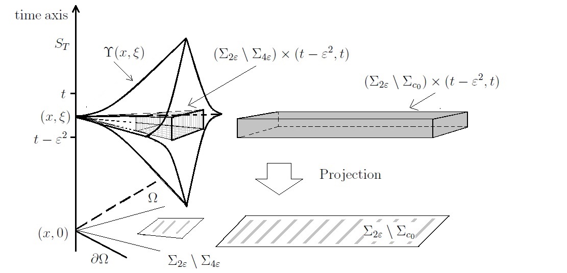
Precisely, a subtle fact observed in Figure 1 will be frequently used in the later sections, which is
| (1.12) |
and
| (1.13) |
where , and is independent of . Then, integrating both sides of the above inequalities with respect to from to , the left-hand sides of and will be controlled by the quantities and , which will further be determined by the given lateral data (see [22, Theorem 4.2.1]). Here we always divide into and , where the region will be good part for related calculations in general.
Next, we will show some important observations on the co-layer type estimates . Again, we only focus ourselves on the estimate of
| (1.14) |
whereas it is not hard to verify . To do so, we consider the following pointwise estimate
for any , which may be found in [20, pp.1148-1149]. Since there holds the following relationship between a parabolic ball and a parabolic nontangential approach region:
where is the point such that . Hence we have the following estimate
| (1.15) |
This together with the parabolic nontangential maximal estimate [22, Theorem 4.2.1] leads to the desired estimate . Consequently, the main procedures in the proof of have been introduced to the reader. We must mention that such the aforemention techniques have already been in Z. Shen’s recent work [21] for elliptic cases.
Innovations originally come from managing to improve the estimate . It is natural to think of the distance function as a weight to increase some integrability in the right-hand side of , as a result of the fact that . Although this weight may lead to some better estimates, such as
it also arises other intractable problems. One of them is to bound the following quantity
by , which urges us to find a weighted Caccioppoli’s inequality in a time-layer region (see Lemma 4.2). Beyond this, we require that the weight functions can pass through the smoothing operators and freely, which has been summarized in Lemmas 2.8, 2.9 and 2.7. As far as the authors have known, they are new established in this paper. Therefore, in technical point of view, the order of in the estimate will come from two sources. One is straightforwardly from the duality method as J. Geng and Z. Shen did in [10], the other is actually attributed to the weight function . Since the duality method has been well illustrated in [10, 27], we do not repeat here.
Up to now, we have shown the main tricks related to the estimates and , and so to . We mention that the estimate may play a fundamental part in further quantitative estimates, such as uniform Hölder estimates and estimates with . This is an active field and some of them have been established through compactness methods (see [11]). We also highly recommend [21] for recent developments in periodic homogenization theory, as well as [1, 2] for a non-periodic setting.
We end this section by two remarks.
Remark 1.3.
We emphasis that the expression in can not be replaced by in [10], even though we are able to establish the weighted-type estimates for in (see Corollary 2.10). In concrete calculations, will serve as a role in eliminating one spatial derivative, by reason of that there is no good way of bounding derivatives of third order. Note that there naturally hold global regularity estimates for and provided as in [10, 19]. By contrast, for a Lipschitz cylinder, we have to rely on some subtle arguments mentioned before.
Remark 1.4.
We point out that the arguments developed in this paper can be extended to other initial-boundary problems, and to the parabolic operators with lower order terms. The crucial estimates actually relies on the symmetry assumption on , while the methods for getting rid of it have been studied in recent work [15], which will possibly illuminate the sharp uniform estimate with regard to smooth cylinders.
2 Preliminaries
2.1 Notation
We first introduce notation for derivatives.
-
1.
is the gradient of with respect to spatial variable, where denotes the spatial derivative of . denotes the Hessian matrix of , where .
-
2.
briefly represents the derivative of with respect to the time variable.
The following notation represents function spaces and weighted-type norms.
- 1.
-
2.
The weighted-type norms are defined by
(2.1) where the weight function may be chosen from and .
2.2 theory
Theorem 2.1.
Suppose that satisfies . Let and with . Then there exists a unique weak solution to satisfying the uniform energy estimate
| (2.2) |
where depends on and .
Proof.
We first prove the existence of weak solution . Following the notation from [7], we define . On account of [7, Theorem 2.9] and [7, Theorem 3.4], there exists such that , and
Let , where , and we have
| (2.3) |
where , and we use the fact that in . Then the source term in belongs to , bounded by . Therefore, the existence of weak solution to is reduced to finding a weak solution for , and it has been done by [8, Theorem 3, pp.378]. The uniqueness of the weak solution may be easily derived by the energy inequality , and this is what we do in next step.
For the equation , it follows from [18, Lemma 2.1, Chapter III] that
where we need to employ the elasticity condition coupled with the first Korn inequality (see [16, pp.371]), and this implies
| (2.4) |
From this estimate, we know that , and this together with [8, Theorem 3, pp.303] and the estimate leads to
where we use the equation and in the second step. We have completed the proof. ∎
Proof of Theorem 1.1. The proof is quite similar to that given for [11, Theorem 3.6] in the case of , which follows from the estimate and Tartar’s test function methods (it actually does not involve any boundary condition or initial data). Thus, without a proof, we straightforwardly show the following facts:
| (2.5) |
where satisfies in . Then we plan to verify on in a trace sense, and for a.e. . It follows from together with the Aubin-Lions-Simon theorem that
| (2.6) |
Also, in view of [8, Theorem 3, pp.303], we have . Our now task is to verify on . Let be a test function, where and satisfying and . By reusing , we have
This gives
where we employ and in the last step. The desired result directly follows from the arbitrary choosing . The next step is to show on . Owing to and , we can derive strongly in , just by noting
This implies on in the trace sense, and we end the proof here. ∎
2.3 Correctors and its properties
Let . Define the correctors associated with the parabolic system by the following cell problem:
| (2.7) |
where , and with 1 in the position. Since there is no boundary term produced by taking integration by parts, it follows from energy inequality [18, pp.139] that
| (2.8) |
By asymptotic expansion arguments the homogenized operator is given by , where and
| (2.9) |
Lemma 2.2.
Let and , and
| (2.10) |
where and . Then the quantity with satisfies two properties:
| (2.11) |
Moreover, there exists such that
| (2.12) |
where depends only on and .
Proof.
See [10, Lemma 2.1]. ∎
2.4 Smoothing operator and its properties
Definition 1.
Fix with . Define a smoothing operator associated with the spatial variable as
| (2.13) |
where . Let satisfy . Define a parabolic smoothing operator as
| (2.14) |
where .
Lemma 2.3.
Let with , then for any we have
| (2.15) | ||||
where depends on and .
Lemma 2.4.
Let , and be given in . Then for any , we have
| (2.16) |
Moreover, if we define
| (2.17) |
with , where , and . Then there holds
| (2.18) |
where depends on and .
Remark 2.5.
Note that there must be by definition. So the symbol is only used to simplify the statements of the lemma, and will not appear in any other place.
Proof.
The estimate is easily observed, and we provide a proof for the sake of completeness. Let be the point such that , and we remark that either or . According to the definition of distance function (see ), it is not hard to see that for any with ,
and interchanging the variable and leads to the same type inequality. This implies the desired estimate .
We now proceed to prove the first estimate in , the main idea is to quantify the difference between and . It is clear to see that
| (2.19) | ||||
where we use the estimate in the last step. Since , we have already proved the first estimate of . An argument similar to the one used in will show the second one in , and we are done. ∎
Lemma 2.6.
Assume . Then we have
| (2.20) | ||||
as well as,
| (2.21) |
where depends on and . Moreover, if , then there holds
| (2.22) |
where depends on and .
Proof.
The estimate follows from the Plancherel theorem immediately, while the estimates and essentially come from the absolute continuity of the integral with respect to a small translation. We will adopt the idea from [10, Lemma 3.2], originally developed by Z. Shen [21]. In view of the Plancherel theorem, the left-hand side of is equal to
| (2.23) |
Since , we have . Hence, the quantity may be controlled by
and this implies the desired estimate through the Plancherel theorem again. By the same token, the estimate is based upon the following estimate
where the pair is in the phase space, produced by the spacial and the time variable, respectively. ∎
Recall the definition of weighted-type norms , and the parabolic distance function is defined in .
Lemma 2.7.
Let be supported in . Then there holds
| (2.24) |
| (2.25) |
for , and
| (2.26) |
where depends on and .
Proof.
We only show the proof in the case of , and the other case follows from the same way. To show , we fix , and it follows from [27, Lemma 3.2] that
| (2.27) |
where is independent of , and integrating the above inequality with respect to from to leads to the desired estimate . Denote
where . Then an argument similar to the one used in Lemma 2.4 shows that
| (2.28) |
since for fixed , there still holds
Hence, the estimate shall lead to the estimate . The proof will not be fully included here, and the similar details will be found in Lemma 2.8.
By the same token, for any fixed , it follows from [27, Lemma 3.3] that
where is independent of , and this implies is true. We have completed the proof. ∎
Lemma 2.8 (Weighted-type inequality I).
Let be supported in . Then for any , there holds
| (2.29) | ||||
and
| (2.30) | ||||
where depends only on and .
Proof.
Concerning the estimates and , the main idea has already been in [27, Lemma 3.2], and we provide a proof for the sake of the completeness. For any and , it follows from Cauchy’s inequality that
| (2.31) | ||||
where we employ the estimate in the last step. To estimate , it suffices to show
| (2.32) | ||||
where we use the estimate in the first inequality, and the second one follows from the Fubini theorem, and the last step is due to . Here the symbol means a cube in with being the center, with as the length of a side.
Adopting the same procedure as we did above, one can derive the estimate without any real difficulty, which is based on the fact
| (2.33) |
and the estimate in the case of . Thus we may end the proof here. ∎
Lemma 2.9 (Weighted-type inequality II).
Let be supported in . Then we have
| (2.34) | ||||
where depends on and .
Proof.
Unlike the method used in the proof of Lemma 2.6, we will employ the arguments similar to that shown in [27, Lemma 3.3] to prove this lemma. Let and , and it is not hard to see that
Then we have
| (2.35) | ||||
For , set . It is clear to see , and
| (2.36) | ||||
due to the fact that for any . Concerning , we reset and . Thus and , and it follows from the estimate that
By the same token, we have
| (2.37) |
Inserting and into the estimate leads to
Then the rest part of the proof of is based upon the Fubini theorem and the estimate , which will be found in [27, Lemma 3.3] and will not be reproduced here. We have completed the whole proof. ∎
Corollary 2.10.
Assume . Then there holds
| (2.38) |
Moreover, if is supported in , then we have
| (2.39) |
where depends on and .
Proof.
We mention that the estimate had been proven in [10, Lemma 3.2] by the Plancherel theorem. Based upon the previous Lemma 2.6, we provide a new proof here, and this method could be applied to the estimate as well.
In view of , it is not hard to see that
Hence, from the above inequality, it follows that
where we use the estimates and in the second inequality, and the estimate in the last one.
Proceeding as in the proof of the estimate , it is not hard to derive the weighted-type one . All the requirements have been established except the following estimate
However, it is could be easily acquired from Lemma 2.4, and we omit the details here. The proof is now complete. ∎
Remark 2.11.
Although Corollary 2.10 has not been employed in this paper, there are two reasons making us feel necessary to write it out. One is that we provide an idea in the proof of , which actually suggests a new way for [10, Lemma 3.2] to avoid using the Fourier transformation method. The other is that from the proof of this corollary, it is clear to see why we fix the undetermined function in by choosing rather than in the later sections.
3 Convergence rates in
Lemma 3.1.
Suppose that with satisfy
| (3.1) |
Let with
| (3.2) |
where is supported in . Then we have
| (3.3) |
where with
| (3.4) | ||||
where and , and with .
Proof.
The proof may be found in [10, Theorem 2.2], and we provide a proof for the sake of the completeness. Observing the equation , we have
| (3.5) | ||||
where is shown as in , and with . The last line of is a good term, and our task is reduced to calculate , and . Recalling Lemma 2.2, it is not hard to see that
| (3.6) |
where we use the equality (ii) in . Then in view of , the right-hand side of may be rewritten by
| (3.7) | ||||
where , and we use the fact that due to the antisymmetry. Again, employing the antisymmetry of , the second line of is equal to
Thus, we have
and this together with the last line of implies the desired formula . The proof is complete. ∎
Theorem 3.2.
Given , and . Let with be the weak solutions to and , respectively. Then by setting in , we have
| (3.8) |
where depends only on and .
Lemma 3.3.
Suppose . Let be given as in and satisfy the problem . Then by choosing in , we may have
| (3.9) | ||||
where depends only on and .
Proof.
Noting that in such that satisfies , it follows from the estimate and the expression that
| (3.10) | ||||
To estimate , we first notice the following fact
Hence, it follows from the estimates , and that
where we also use the fact that is supported in , and .
Since there holds the following identity
| (3.11) |
we then obtain
| (3.12) | ||||
where we use the estimates in the first inequality again, and the second one is due to
| (3.13) |
We now proceed to study , and it follows from the first estimate in that
| (3.14) |
By observing that
it is not hard to derive
| (3.15) |
from the second estimate in . Based upon a similar fact that
| (3.16) |
using the estimates and again, we arrive at
| (3.17) |
Consequently, plugging , , and back into leads to the desired result, and we have completed the proof. ∎
Lemma 3.4.
Suppose , and . Let be a weak solution of . Then for any , we have the following interior estimates
| (3.18) | ||||
where depends on , as well as,
| (3.19) |
where will blow up as . Moreover, there also holds a global estimate
| (3.20) |
where depends on and .
Remark 3.5.
In fact, the estimate could be improved from the point of view in the homogenization theory, and one may easily derive from the estimates and that
by noting that and are lower semi-continuous with respect to the weak convergence and to the convergence, respectively.
Proof.
The estimate is known as Caccioppoli’s inequality. Let be a test function, where . By the divergence theorem, we have
On account of the elasticity assumption and Young’s inequality, there holds
| (3.21) |
where we exactly carry out a following simple computation:
and the notation denotes the transpose of matrix .
Here, we concretely choose to be the cut-off function, where in , outside and . Hence, we obtain
and then take integral on the both sides from to . The desired estimate immediately follows from Cauchy’s inequality.
The estimate has been proved in [26, Theorem 3.4.1] in detail, so the proof will not be repeated here.
We now turn to address the estimate . Since in , taking as the text function and then integrating by parts, we have
Here we assume for a movement to make the above identity reasonable. By the elasticity assumption , we have
| (3.22) |
where the symbol denotes the a tangential derivative. Here we also employ the following Korn inequality:
Then it is fine to split into and , and they satisfy
respectively. Thus, concerning , the estimate coupled with the Gronwall’s inequality yields
| (3.23) |
For , the estimate together with Cauchy’s inequality and the trace theorem gives
From Gronwall’s inequality, it follows that
| (3.24) | ||||
where we use the fact that (see [22, Lemma 4.3.13]) in the second step.
Consequently, the desired estimate follows from the estimates and , and we completed the proof. ∎
Lemma 3.6.
Suppose that satisfies and . Assume , and . Let be the weak solution of . Then we have the lateral-layer type estimate
| (3.25) |
and time-layer type estimate
| (3.26) |
and co-layer type estimates
| (3.27) |
where depends at most on and .
Proof.
The main idea in the proofs is analogous to that applied to elliptic operators, and we refer the reader to [21, 27] for the original idea. We first address the spatial-layer type estimate . Due to the linearity of the equation , we may divide the solution into three parts, which means and satisfy the following equations (i), (ii), (iii), respectively.
where , and is a new domain with boundary, and denotes the lateral of . Here is a 0-extension to such that in and in , while is a -extension to satisfying in and .
We note that the existences of and have be shown in [22, Theorem 4.2.1], and the second equality in (ii), as well as in (iii), should be understood in the sense of nontangential convergence.
Concerning the equation (i), it follows from the regularity of initial-Dirichlet problem (see [8, Section 7.1.3]) that
and this together with the energy estimate
gives the following estimate
| (3.28) | ||||
where depends at most on and . Recalling the definition of , for any and , it follows from the trace theorem that
where is independent of and . By the co-area formula, we have
Integrating from to with respect to the time variable and then taking the square root, it holds
| (3.29) | ||||
where we use the estimate in the last inequality.
We now proceed to study the equations (ii) and (iii). Due to the work of Z. Shen’s, it is well known that
| (3.30) |
(see [22, Lemma 4.3.13]), which may be derived from the so-called Rellich identity. By the way, the original work in the case of traces back to R. Brown (see [6, Section 3]). Hence, on account of [22, Theorem 4.2.1] we have
| (3.31) | ||||
where we employ the equivalence in the second inequality. From the trace theorem in space variable, it is not hard to see that
where we use the estimate in the last step. Thus, the third line of will be controlled by
For the ease of the statement, let . Then we have known and
| (3.32) |
and this implies
| (3.33) | ||||
Thus, combining the estimates and , we have proved the spatial-layer type estimate .
We now turn to investigate the time-layer type estimate . Due to the estimate , the problem is reduced to estimate the following terms:
| (3.34) |
The easiest one is
| (3.35) |
where we employ the estimate . Then we address the first term in . Recalling , there exists such that
where we use the trace theorem for and the definition of the maximal function of in the second inequality. Then integrating both sides of the above inequality with respect to from to , we have
| (3.36) |
where we use the estimates and .
Now, we focus on the last term in . Noting that in , we acquire
| (3.37) |
It suffices to estimate the first term in the right-hand side of . Since using leads to
| (3.38) | ||||
the problem is reduced to estimate the last term of . And we obtain
where , and we use the interior estimates [20, Lemma 1] and in the second step, and the last one follows from the definition of nontangential maximal function and the estimate . By integrating with respect to from to , it is shown that
and this together with the estimates and gives
| (3.39) |
Hence, plugging the estimates and (3.39) back into the estimate , we obtain
| (3.40) |
and this verifies the desired time-layer-type estimate .
The rest of the proof is devoted to the so-called co-layer type estimate . Since in , it is sufficient to prove the estimate for the quantity
In view of , the above one could be controlled by
| (3.41) | ||||
where we use the estimate . From the interior estimate and the global estimate , it follows that
| (3.42) |
We proceed to estimate by the method analogous to that used above. However, we have to, in advance, remove one more order derivative from , carefully. Due to the interior regularity estimate [20, Lemma 1] and the Sobolev imbedding theorem (see [20, pp.1148-1149]), there holds
| (3.43) |
for any , where . We remark that the existence of in fact comes from layer potential theory concerning parabolic equations, the key idea from R. Brown [6] is that extending to a caloric function which is still caloric on . Roughly speaking, since the estimate is just an interior estimate and the extension of is still determined by given data and , here we may regard as being a solution of in .
Hence, in view of the co-area formula, we obtain
| (3.44) | ||||
where we use the estimate in the last step. Combining the estimates , and gives
Until now, we have proved the desired estimate , and the whole proof is complete. ∎
4 Convergence rates in
In order to accelerate the convergence rate, we shall employ the so-called duality methods. To do so, we first consider the adjoint initial-Dirichlet problems: given , let and be the weak solution to
respectively. Here is the adjoint operator of . By the symmetry condition , let and , which exactly right solve the initial-Dirichlet problems
We mention that and are corresponding correctors and dual correctors associated with , respectively. It is clear to see that the adjoint problems will obey Theorems 2.1, 3.2 as well.
Lemma 4.1 (Duality lemma).
Let be given in by choosing , where are weak solution of and , respectively. For any , we assume that with are the weak solutions to the adjoint problems and , respectively. Then we have
| (4.1) |
where is shown in . Moreover, if we assume
| (4.2) | ||||
then there holds
| (4.3) | ||||
where depends on and .
Proof.
First, it is not hard to see that the equality follows from integrating by parts
where are weak solutions of and , respectively, and we employ the initial-boundary conditions on in the second step, and in the last one.
Let denote its periodic parts for simplicity of presentation. Thus, observing we have
| (4.4) | ||||
Before proceeding further, we want to show the main ideas on accelerating the convergence rates. The key step is to replace by
| (4.5) | ||||
Here is given by , and it follows from Theorem 3.2 that
| (4.6) |
Observing again, all the terms will produce except for the second term in a co-layer type estimate, and this naturally arouse the distance function playing a role as a weight function in the following calculation.
To estimate , we divide it into two parts:
We first handle as below
| (4.7) |
where we replace by in the last step, and use the fact that the last two terms of vanish in since they are supported in . We then turn to study . It also decomposes into four parts:
| (4.8) | ||||
| (4.9) |
and
| (4.10) | ||||
By Cauchy’s inequality, it is not hard to see that the expression is controlled by
where we use the estimates and in the inequality, and this together with partially produces the first term in the right-hand side of . Concerning , using the same argument as in the proof of Lemma 3.3 we can easily obtain
| (4.11) | ||||
where we employ the estimates , . Hence, it is apparent to see that is governed by the first term in the right-hand side of .
We proceed to address , which is dominated by
Then applying the weighted-type inequalities and , we obtain
Due to the fact , we arrive at
and this exactly gives the second term in the right-hand side of . Up to now, we have completed the estimates for . Also, the above proof actually have shown the following estimates
| (4.12) |
and
| (4.13) |
Proceeding to study as in the proof for , we first have
and then by the estimates , , , , and , we acquire
To estimate , it suffices to estimate
Thus, it follows from the estimates and that
| (4.14) |
and from the estimates and that
| (4.15) | ||||
Combining the estimates , , and gives the corresponding estimate for , which partially forms the right-hand side of .
For , using the same argument as before, we are ready to establish estimates for
respectively. Recalling the crucial observation , the estimate for actually have been shown in the proof of Lemma 3.3, which is
| (4.16) |
Regarding , employing again, it follows from the estimates and that
| (4.17) |
Thus, the estimates , , and lead to
and this ends the proof. ∎
Lemma 4.2 (Weighted Caccioppoli’s inequality).
Let be a weak solution of in , and the distance functions are defined in and , respectively. Then for any , we have the following weighted-type estimate
| (4.18) | ||||
where depends on .
Proof.
We will carry out the proof by suitable modification to the one for the estimate in Lemma 3.4. Set . In view of the estimate , we choose , where the distance function is defined in , and is a cut-off function satisfying in , and outside with . Then, putting
into the estimate , for any fixed , we have
Then integrating the both sides of the above inequality with respect to from to , and we have proved the following estimate:
| (4.19) | ||||
Our task now is to analyze the concrete behavior of the distance function in the integrals and . Since for any , we have
| (4.20) |
By noting that
and in , the integral is just equal to
| (4.21) |
while the integral will produce two terms:
| (4.22) |
We ends the proof by substituting the expressions , and for , and in the estimate , respectively. Obviously, the first term of could be absorbed by , and we have completed the whole proof. ∎
Lemma 4.3 (Improved lemma).
Assume the same conditions as in Lemma 3.6. Let be the weak solution of with , and satisfying
Then we have
| (4.23) |
and
| (4.24) |
where depends on and .
Proof.
First, we will address the estimate . Recalling and the definition of the distance function (see ), it is not hard to see that
where we employ the estimates and in the last step.
We now turn to study the estimate . Using the same arguments as in the proof of the estimate to prove the first two quantities in the left-hand side of , it suffices to bound
by
recalling , and together with is shown in the proof of Lemma 3.6. Obviously, it follows from the estimates and that
Thus, our task is reduced to estimate . On account of the estimate , we obtain
by noting that . This together the estimate for implies the estimate
| (4.25) |
Since in , to estimate
is reduced to the estimate .
So, the remainder thing is to investigate the quantity
which will be divided by four parts:
and
where we note that in .
Since in , we can easily have
| (4.26) |
from the estimate . To estimate , we first define the radical maximal function as
| (4.27) |
for any and , where are a family of bi-Lipschitz maps (see for example [17, 27]). Hence, by co-area formula, it is not hard to derive
| (4.28) | ||||
where we use the fact that in the second inequality, and the third one involves two important things: one is
(see [29, Lemma 2.24]), the other is the observation that on . The last inequality of follows from the estimates and .
We now turn to and . In fact, by changing variable, the study on may be reduced to investigate . Thus we focus our minds on . First of all, it is better to slip in two parts:
It is clear to see that we can adopt the same arguments used in to derive
| (4.29) |
and we do not reproduce the details here. Concerning , set and , which follows from . Hence, we obtain
| (4.30) |
provided that
| (4.31) |
Hence, the problem is reduced to estimate . It follows from the weighted Caccioppoli’s inequality that
| (4.32) | ||||
by noting that in . Since there holds
for any , the second line of is reduced to estimate the quantity
Hence, following the methods employed in the estimate we arrive at
where . Integrating the both sides of the above inequality with respect to from to , we consequently reach
| (4.33) |
through the estimates and .
An argument similar to the one used in the estimate shows that
| (4.34) |
where we note that . Besides, adopting the idea similar to the one used in the estimate , it is not hard to derive
| (4.35) |
Thus, collecting the estimates , and leads to the desired estimate . Finally, the estimates and give
and this together with the estimates and implies
Up to now, we have proved the estimate and completed the whole proof. ∎
Proof of Theorem 1.2. First of all, we may assume . On account of Lemmas 4.1 and 4.3 and 3.6, for any , it is not hard to derive from the estimates , and together with , that
| (4.36) | ||||
where we also employed the estimate in the computation, which shows that
| (4.37) |
Since
it suffices to estimate
Form the estimates and , we can assert that the above two quantities will be determined by . This together with the estimate and implies
We have completed all the proof. ∎
Acknowledgements
The first author wants to express his sincere appreciation to Professor Zhongwei Shen for his constant guidance and encouragement. The first author was supported by the National Natural Science Foundation of China (Grant NO.11471147). The second author was supported by the National Natural Science Foundation of China (Grant NO.11571020).
References
- [1] S. Armstrong, C. Smart, Quantitative stochastic homogenization of convex integral functionals, Ann. Sci. Éc. Norm. Supér., (to appear).
- [2] S. Armstrong, Z. Shen, Lipschitz estimates in almost-periodic homogenization, Comm. Pure Appl. Math. 69(2016), no.10, 1882-1923.
- [3] M. Avellaneda and F. Lin, Compactness methods in the theory of homogenization, Comm. Pure Appl. Math. 40(1987), no.6, 803-847.
- [4] A. Bensoussan, J.-L. Lions, and G.C. Papanicolaou, Asympotic Analysis for Periodic Structures, Studies in Mathematics and its Applications, North Holland, 1978.
- [5] M. Sh. Birman, T. Suslina, Second order periodic differential operator. Threshold properties and homogenization, Algebra i Analiz 15(2003), no. 5, 1-108; English transl., St. Petersburg Math. J. 15(2004), no. 5, 639-714.
- [6] R. Brown, The method of layer potentials for the heat equation in Lipschitz cylinders, Amer. J. Math. 111(1989), no.2, 339-379.
- [7] M. Costabel, Boundary integral operators for the heat equation, Integral Equations Operator Theory 13(1990), no.4, 498-552.
- [8] L.C. Evans, Partial Differential Equations, second ed., Graduate Studies in Mathematics 19. American Mathematical Society, Providence, RI, 2010.
- [9] J. Geng, Z. Shen, Uniform regularity estimates in parabolic homogenization, Indiana Univ. Math. J. 64(2015), no.3, 697-733.
- [10] J. Geng, Z. Shen, Convergence rates in parabolic homogenization with time-dependent coefficients, J. Funct. Anal. 272(2017), no.5, 2092-2113.
- [11] J. Geng, Z. Shen, L. Song, Boundary Korn inequality and Neumann problems in homogenization of systems of elasticity, Arch. Ration. Mech. Anal. 224(2017), 1205-1236.
- [12] G. Griso, Error estimate and unfolding for periodic homogenization, Asymptot. Anal. 40(2004), 269-286.
- [13] G. Griso, Interior error estimate for periodic homogenization, Anal. Appl. (Singap.) 4(2006), no.1, 61-79.
- [14] S. Gu, Convergence rates in homogenization of Stokes systems, J. Differential Equations 260(2016), no.7, 5796-5815.
- [15] S. Gu, Q. Xu, Optimal boundary estimates for Stokes systems in homogenization theory, arXiv:1612.06042v1,(2016).
- [16] V.V. Jikov, S.M. Kozlov, O.A. Oleinik, Homogenization of Differential Operators and Integral Functionals, Springer-Verlag, Berlin, 1994.
- [17] C.E. Kenig, F. Lin, Z. Shen, Convergence rates in for elliptic homogenization problems, Arch. Ration. Mech. Anal. 203(2012), no.3, 1009-1036.
- [18] O.A. Ladyzenskaja, V.A. Solonnikov, N.N. Uralceva, Linear and Quasilinear Equations of Parabolic Type, (Russian) Translated from the Russian by S. Smith, Translations of Mathematical Monographs, Vol.23 American Mathematical Society, Providence, RI,1968.
- [19] Yu.M. Meshkova, T.A. Suslina, Homogenization of initial boundary value problems for parabolic systems with periodic coefficients. Appl. Anal. 95(2016), no.8, 1736-1775.
- [20] Schauder and estimates for parabolic systems via Campanato spaces, Comm. Partial Differential Equations 21(1996), no.7-8, 1141-1175.
- [21] Z. Shen, Boundary estimates in elliptic homogenization, Anal. PDE 10(2017), 653-694.
- [22] Z. Shen, Boundary value problems for parabolic Lamé systems and a nonstationary linearized system of Navier-Stokes equations in Lipschitz cylinders, Amer. J. Math. 113(1991), no.2, 293-373.
- [23] Z. Shen, J. Zhuge, Boundary layers in periodic homogenization of Neumann problems, Comm. Pure Appl. Math. (accepted).
- [24] T.A. Suslina, Homogenization of the Dirichlet problem for elliptic systems: -operator error estimates, Mathematika 59(2013), no.2, 463-476.
- [25] T.A. Suslina, Homogenization of the Neumann problem for elliptic systems with periodic coefficients, SIAM J. Math. Anal. 45(2013), no.6, 3453-3493.
- [26] Z. Wu, J. Yin, C. Wang, Elliptic & Parabolic Equations, World Scientific Publishing Co. Pte. Ltd., Hackensack, NJ, 2006.
- [27] Q. Xu, Convergence rates for general elliptic homogenization problems in Lipschitz domains, SIAM J. Math. Anal. 48(2016), no.6, 3742-3788.
- [28] Q. Xu, Convergence reates and estimates in homogenization theory of Stokes systems in Lipschitz domains, J. Differential Equations 263(2017), no.1, 398-450.
- [29] Q. Xu, Uniform regularity estimates in homogenization theory of elliptic systems with lower order terms on the Neumann boundary problem, J. Differential Equations 261(2016), no.8, 4368-4423.
- [30] V.V. Zhikov, S.E. Pastukhova, On operator estimates for some problems in homogenization theory, Russ. J. Math. Phys. 12(2005), no. 4, 515-524.