Signatures of an $S_{3}$-Orbifold Higgs Model

Abstract

The lack of new physics at the LHC has sparked renewed interest in theories of neutral naturalness, in which the Standard Model partners required for naturalness carry no Standard Model charge. The Twin Higgs was the first of these theories to be introduced, but recent work has demonstrated it is only an isolated example in a large class of “orbifold Higgs” models. In this work we study an orbifold Higgs model resulting from the orbifold projection by the non-abelian group $S_{3}$. A model with multiple sectors uncharged under the SM emerges. Constraints are placed on the model from Higgs phenomenology and the prospects of finding evidence at colliders are discussed.

1 Introduction

The discovery of the Higgs boson[1, 2] has provided us with the last piece needed to complete the Standard Model (SM). Due to radiative corrections to the Higgs mass term, the SM requires an extreme fine tuning in order to keep the weak scale much smaller than the Planck scale. With the belief that such a tuning in nature is unnatural, many solutions have been proposed to eliminate the large quadratic corrections to the Higgs mass, thus eliminating the hierarchy problem. Supersymmetry and compositeness are prime examples of such theories, but current null search results for SM partners are now forcing many of these models into finely tuned territory. The fine tuning that is necessary to create a hierarchy between the weak scale and the scale which new physics appears is called the little-hierarchy problem[3].

The Twin Higgs[4, 5] is a solution to the little-hierarchy problem where the SM Higgs is played by the role of a pseudo-Goldstone boson. The SM fields are joined by a set of partners called “twin” states. These SM partners differ in comparison to those in supersymmetry in that they carry no SM charge. This would make current searches for partner states to the SM especially challenging and may explain current null search results at the LHC. A discrete $\mathds{Z}_{2}$ symmetry that interchanges the SM fields with the twin states then ensures gauge, Yukawa, and scalar self interactions must be equivalent in the SM and twin sectors. This protects the pseudo-Goldstone Higgs against the quadratic corrections the Higgs mass term receives in the SM. Typically for cutoff scales $\Lambda\sim 5-10\mbox{ TeV}$ these models do not suffer from any major fine tuning. At higher scales a stronger mechanism such as compositeness or SUSY may keep the weak scale natural to the Planck scale as demonstrated in UV completions of the Twin Higgs[6, 7, 8, 9, 10, 11, 12, 13, 14].

Other theories of neutral naturalness have since been introduced[15, 16, 17, 18, 19], including recent work which has demonstrated that the Twin Higgs is only the simplest example in a large class of orbifold Higgs models[20, 21]. In orbifold Higgs models, the Higgs is protected by an accidental symmetry resulting from an orbifold reduction of a larger symmetry via some discrete group. These models also generically give rise to states that are uncharged under the SM. The orbifold interpretation also lends itself nicely in creating UV complete models as geometric orbifolds of some higher dimensional space.

In this paper we explore one of these orbifold Higgs models arising from a non-abelian orbifold pattern, namely $S_{3}$. Like the Twin Higgs this produces hidden sectors, one SM-like in structure and another exotic sector with an $SU(6)$ color group, $SU(4)$ weak isospin group, and an $SU(2)$ flavor symmetry among the Higgs and top partners. Though the model has been specified in the original orbifold Higgs papers, the details of the experimental signatures have yet to be carried out. In this paper we explore the phenomenology of the $125\mbox{ GeV}$ SM-like Higgs generated by the model and compare results to the signatures predicted in the Twin Higgs.

In the next section we will review the features of the Twin Higgs. Following this the formalism behind field theory orbifolds will be given as a necessity to understand how orbifold Higgs models are constructed. The $S_{3}$-orbifold Higgs will then be presented and we’ll demonstrate how a natural SM-like Higgs emerges from the model. Section 5 will analyze some of the phenomenology and compare the results to the Twin Higgs and section 6 will contain our conclusions.

2 Twin Higgs Review

We will now take a moment to review the Mirror Twin Higgs[4]. We begin with a complex scalar, $H$, which transforms as a fundamental of a global $SU(4)$ symmetry. The scalar potential is given by,

$$V=-m^{2}|H|^{2}+\lambda|H|^{4}$$ (2.1)

where $m^{2}>0$. $H$ picks up a vacuum expectation value (vev), $|\langle H\rangle|\equiv\frac{f}{\sqrt{2}}$, and the global symmetry is broken to $SU(4)\rightarrow SU(3)$ yielding 7 massless Goldstone bosons.

We now explicitly break the global $SU(4)$ by gauging the subgroup $SU(2)_{A}\times SU(2)_{B}\subset SU(4)$ such that H transforms as $H^{T}=(H_{A}\,\,H_{B})$. After gauging this symmetry the global $SU(4)$ symmetry is still an accidental symmetry of the tree level potential. In general, radiative corrections to the potential will not be invariant under the accidental $SU(4)$. For instance the Higgs gauge interactions generate terms such as

$$\Delta V\sim\frac{9\Lambda^{2}}{16\pi^{2}}\left(g_{A}^{2}|H_{A}|^{2}+g_{B}^{2}|H_{B}|^{2}\right),$$ (2.2)

where we have used a uniform hard cutoff to regulate the integrals. This introduces mass terms for the Goldstones that are quadratically sensitive to the cutoff. We can eliminate this by introducing a discrete $\mathbb{Z}_{2}$ symmetry, dubbed twin-parity. This symmetry exchanges the gauge fields and $H_{A}\leftrightarrow H_{B}$ which enforces that the gauge couplings are equal, $g\equiv g_{A}=g_{B}$. Now,

$$\Delta V\sim\frac{9g^{2}\Lambda^{2}}{16\pi^{2}}\left(|H_{A}|^{2}+|H_{B}|^{2}\right)=\frac{9g^{2}\Lambda^{2}}{16\pi^{2}}\left(|H|^{2}\right)$$ (2.3)

which is an $SU(4)$ invariant. Thus the quadratic divergences do not contribute to the masses of the Goldstone bosons. From here we can create twin copies of the fermions and gluons and extend twin parity to the twin gluons and fermions. This will eliminate the quadratic divergences due to the Yukawa interactions. The Higgs mass term and quartic interactions arise from $SU(4)$ breaking terms stemming from the one-loop effective potential.

Without additional soft terms added to the potential neither sector is suited to be identified with the SM sector as the Higgs would be equally aligned with both $A$ and $B$ sectors. This would lead to a $1/\sqrt{2}$ suppression in the couplings of the Higgs to the SM which isn’t consistent with experiment. To identify the $A$-sector with the SM we can add $V_{soft}=\mu|H_{A}|^{2}$ to the potential which softly break twin parity. Tuning the soft term, $\rho$, against the $SU(4)$ breaking order parameter, $f$, will suppress the $A$-sector Higgs couplings to $B$-sector states by $\sin(v/f)$ where v is the vev of the SM Higgs. For $v\ll f$ this provides a phenomenologically viable scenario where the SM is associated with the $A$-sector. We will see in the following sections how the Twin Higgs paradigm can be generalized by way of the orbifold Higgs and how the quadratic divergences are eliminated (or at least suppressed) in general orbifold Higgs theories.

3 Building an Orbifold Higgs Model

In this section we will briefly review field theory orbifolds which will be vital to understanding orbifold Higgs models. For a more detailed approach of what follows we refer the reader to ref. [21, 22].

3.1 Field Theory Orbifolds

Let’s begin with some initial field theory, called the parent theory, which has some global or gauge symmetry, $G$. To orbifold the parent symmetry by some discrete group, $\mathcal{G}$, we must study the action of $\mathcal{G}$ on $G$. This requires that we first embed $\mathcal{G}$ into the parent theory which we will do through the regular representation embedding. The fields in the parent theory that are left invariant under the action under $\mathcal{G}$ will be those that comprise the daughter theory and all other states are projected out.

As an example, consider a parent theory consisting of a scalar, $H$, which transforms as a bifundamental of a gauged $SU(\Gamma N)$ and global $SU(\Gamma F)$, where $F,N\in\mathds{N}$, as shown in Figure 1 . We’ll then take our discrete group, $\mathcal{G}$, to be of order, $|\mathcal{G}|=\Gamma$.

	$SU(\Gamma N)$	$SU(\Gamma F)$
$H$	$\square$	$\overline{\square}$

Figure 1: Transformation properties of the scalar field $H$ in the parent theory.

We now need to determine the orbifold of the parent theory by $\mathcal{G}$. First, we express $\mathcal{G}$ in the regular representation which has the following well known decomposition,

$$\begin{array}[]{cc}\gamma^{s}_{R}=\bigoplus\limits_{\alpha=1}^{n_{\mathcal{G}}}\mathds{1}_{d_{\alpha}}\otimes r^{s}_{\alpha}&\hskip 14.22636pts\in 1...\Gamma.\end{array}$$ (3.1)

Here, $s$ labels the elements of the group, $r_{\alpha}$ denotes the irreducible representations of $\mathcal{G}$ with relative dimension $d_{\alpha}$, and $\alpha$ sums over the $n_{\mathcal{G}}$ irreducible representations. To embed $\mathcal{G}$ into $SU(N\Gamma)$ we take the direct product of the N-dimensional identity and regular representation yielding,

$$\gamma^{s}_{N}\equiv\mathds{1}_{N}\otimes\gamma^{s}_{R}=\bigoplus\limits_{\alpha}\mathds{1}_{Nd_{\alpha}}\otimes r_{\alpha}^{s}.$$ (3.2)

We can now study the transformation properties of the fields in the parent theory under action of $\gamma_{N}$ and project out all fields not invariant under the action. For fields transforming in the adjoint representation, the invariant states are those satisfying,

$$A=\gamma^{s}_{N}\,A\,\left(\gamma^{s}_{N}\right)^{\dagger}$$ (3.3)

for all $s\in\{1...\Gamma\}$.The orbifold of $SU(\Gamma N)$ by $\mathcal{G}$ reduces the symmetry to a direct product of smaller symmetry groups in the daughter theory, namely

$$SU(\Gamma N)\longrightarrow\left(\prod\limits_{\alpha=1}^{n_{\mathcal{G}}}SU(d_{\alpha}N)\right)\otimes\left(U(1)\right)^{n_{\mathcal{G}}-1}.$$ (3.4)

To find the invariant components of fields transforming in the fundamental representation it’s convenient to construct projection operators. For the field $H$ transforming as a bifundamental of $SU(\Gamma N)\times SU(\Gamma F)$ the projection operator takes the form,

$$P_{R}=\frac{1}{\Gamma}\sum\limits^{\Gamma}_{s=1}\gamma_{N}^{s}\otimes(\gamma_{F}^{s})^{*},$$ (3.5)

where $P_{R}$ acts on the left of $H$. This procedure will in general leave us with a daughter theory with non-canonically normalized kinetic terms with rescaling related to the dimension of the representation, $d_{\alpha}$. Requiring normalized kinetic terms in the orbifold daughter theory induces a rescaling of the interactions of the daughter theory. Scalar masses, $m$, and double-trace quartic interactions $\lambda$ in the parent theory don’t get rescaled in the daughter, gauge couplings, $g$, and yukawas, $y$, of the parent get rescaled by $1/\sqrt{d_{\alpha}}$, and single trace quartics get rescaled by $1/d_{\alpha}$.

3.2 Orbifold Higgs

We can now construct orbifold Higgs models. We begin with a parent theory consisting of a complex scalar, $H$ and fermions, $Q$ and $U$ which transform as bifundamentals of a gauged $SU(2\Gamma)\times SU(3\Gamma)$ and global $SU(\Gamma)$ flavor symmetry. As before, $\Gamma$ will be taken to be the order of the discrete group, $\mathcal{G}$, used to construct the daughter theory. The matter content is shown in Table 3 and a quiver diagram in Figure 3 .

Figure 2: Quiver diagram of the parent theory. Circular nodes are identified with gauge symmetries and square nodes with flavor symmetries.

	$SU(3\Gamma)$	$SU(2\Gamma)$	$SU(\Gamma)$
$H$	$1$	$\square$	$\overline{\square}$
$Q$	$\square$	$\overline{\square}$	$1$
$U$	$\overline{\square}$	$1$	$\square$

Figure 3: Matter fields in the parent theory.

The scalar potential of the parent theory including the Yukawa interactions is given by

$$V_{P}\supset-m^{2}|H|^{2}+\lambda\left(|H|^{2}\right)^{2}+yQHU.$$ (3.6)

From here we follow the orbifold procedure sketched out above to project out the invariant states of the parent theory. The parent theory will descend to a daughter theory which can be described by a quiver diagram with $n_{\mathcal{G}}$ sets of disconnected nodes, each of which resemble the original structure of parent theory as seen in Figure 4. Each disconnected diagram corresponds to a distinct sector charged only under the gauge fields in it’s own sector .

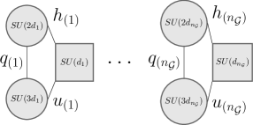
Figure 4: Quiver diagram of the daughter theory resulting from the orbifold reduction of the parent theory.

The potential of the daughter theory takes the form,

$$V_{d}\supset-m^{2}\sum\limits_{\alpha=1}^{n_{\mathcal{G}}}|h_{\alpha}|^{2}+\lambda\left(\sum\limits_{\alpha=1}^{n_{\mathcal{G}}}|h_{\alpha}|^{2}\right)^{2}+\sum\limits_{\alpha=1}^{n_{\mathcal{G}}}\frac{y}{\sqrt{d_{\alpha}}}q_{\alpha}h_{\alpha}u_{\alpha}.$$ (3.7)

The scalar quartic interactions in the daughter theory allows interactions between fields in each sector, not unlike in the Twin Higgs. Note the tree level scalar potential inherits an accidental $SU(2\Gamma)$ symmetry. There is also a residual discrete symmetry in the scalar sector equivalent to the symmetry group leaving the tuple $\{d_{1},d_{2},...,d_{n_{\mathcal{G}}}\}$ invariant. These accidental symmetries may however be broken by radiative corrections due the gauge and Yukawa interactions.

Solving for the leading order radiative corrections to the scalar potential we find,

$$V^{(1)} \supset \frac{\Lambda^{2}}{16\pi^{2}}\left(-6y^{2}+3g_{2}^{2}+(4\Gamma+2)\lambda\right)\left(\sum_{\alpha=1}^{n_{\mathcal{G}}}|h^{(\alpha)}|^{2}\right)$$ (3.8)

$$- \frac{3g_{2}^{2}}{64\pi^{2}}\left(\sum_{\alpha=1}^{n_{\mathcal{G}}}\frac{1}{d_{\alpha}^{2}}|h^{(\alpha)}|^{2}\right)\Lambda^{2}.$$ (3.9)

Note the corrections in the first line share the accidental $SU(2\Gamma)$ symmetry of the tree level potential. One may have naively expected the quark yukawas to spoil this accidental symmetry but there is a fortunate cancelation of the rescaled couplings with the extra color factors. It is only the gauge interactions at leading order which spoil the accidental $SU(2\Gamma)$ symmetry and can contribute to the masses of the would be Goldstones.

The most simple example of an orbifold Higgs is to take the discrete group $\mathcal{G}=\mathds{Z}_{2}$. We would then begin with a parent theory with fields transforming under $SU(6)\times SU(4)$ gauge groups and a $SU(2)$ global symmetry. Upon orbifolding this theory by $\mathds{Z}_{2}$ the parent theory would descend to a daughter theory with two sectors, each charged under a copy of $SU(3)\times SU(2)$ . This is nothing more but the Twin Higgs! The tree level potential of the daughter theory has the desired accidental $SU(4)$ global symmetry and a discrete symmetry of $\mathds{Z}_{2}$ which arises as a consequence of the orbifold reduction of the parent theory whereas in the Twin Higgs it was posited as a means to eliminate quadratic divergences.

4 $S_{3}$-Orbifold Higgs

With the formalism developed we are now equipped to build up the $S_{3}$ orbifold Higgs model. We begin with the potential of the parent theory

$$V_{P} = -m^{2}|H|^{2}+\lambda\left(|H|^{2}\right)^{2}+yQHU$$ (4.1)

where the fields transform as bifundamentals under a $SU(18)\otimes SU(12)$ gauge symmetry and a global $SU(6)$ flavor symmetry.

We will now construct the daughter theory using $\mathcal{G}=S_{3}$ which has 3 irreducible representations: one dimensional trivial and sign representations, and a single two dimensional representation. It follows that we expect three different sectors each charged under its own gauge groups, two of which will look standard model like in structure, and a third exotic sector with larger gauge groups and a residual flavor symmetry. The quivers of the parent and daughter theories are given in Figure 5. The invariant combinations of the parent fields that survive the orbifold projection and comprise the daughter theory of the $S_{3}$-orbifold Higgs model were worked out and are given in ref. [21].

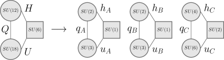
Figure 5: Quiver diagram of the parent and daughter theory resulting from the $S_{3}$-orbifold reduction. The trivial $SU(1)$ nodes are drawn only to demonstrate the connection to the parent theory.

The tree level Higgs potential of the daughter theory is then

$$V^{(0)}_{d} = -m^{2}\left(|h_{A}|^{2}+|h_{B}|^{2}+|h_{C_{1}}|^{2}+|h_{C_{2}}|^{2}\right)$$ (4.2)

$$+ \lambda\left(|h_{A}|^{2}+|h_{A}|^{2}+|h_{C_{1}}|^{2}+|h_{C_{2}}|^{2}\right)^{2}$$ (4.3)

$$+ y\bar{q}_{A}h_{A}u_{A}+y\bar{q}_{B}h_{B}u_{B}+\frac{y}{\sqrt{2}}\bar{q}_{C}h_{C_{1}}u_{C_{1}}+\frac{y}{\sqrt{2}}\bar{q}_{C}h_{C_{2}}u_{C_{2}}.$$ (4.4)

We use the subscripts $C_{1}$ and $C_{2}$ to distinguish the residual $SU(2)$ flavor symmetry. Note the factors of $1/\sqrt{2}$ in the c-sector Yukawa interactions. This comes from the rescaling of terms related to the relative dimension of the irreducible representation.

We now need to include the radiative corrections which will allow us to study the vacuum alignment. The dominant contribution to the one-loop effective potential comes from the top loops,

$$V^{(1)}_{d} \supset \frac{3y^{4}}{16\pi^{2}}\left[|h_{A}|^{4}\log\left(\frac{\Lambda^{2}}{y^{2}|h_{A}|^{2}}\right)+|h_{B}|^{4}\log\left(\frac{\Lambda^{2}}{y^{2}|h_{B}|^{2}}\right)\right.$$ (4.5)

$$+ \left.\frac{1}{2}|h_{C_{1}}|^{4}\log\left(\frac{\Lambda^{2}}{\frac{y^{2}}{2}|h_{C_{1}}|^{2}}\right)+\frac{1}{2}|h_{C_{2}}|^{4}\log\left(\frac{\Lambda^{2}}{\frac{y^{2}}{2}|h_{C_{2}}|^{2}}\right)\right].$$ (4.6)

Adding this contribution to the tree level scalar potential we find that $|\langle h_{A}\rangle|^{2}=|\langle h_{B}\rangle|^{2}=\frac{1}{2}|\langle h_{C_{1}}\rangle|^{2}=\frac{1}{2}|\langle h_{C_{2}}\rangle|^{2}=\frac{1}{2}\frac{m^{2}}{6\lambda+\delta}\equiv\frac{1}{12}f^{2}$. At this point none of sectors can be identified with the SM-like sector due to the fact that the weak scales aren’t adequately separated causing this Higgs to be not well aligned with the SM sector.

To remedy this we add a soft term of the form,

$$V_{soft} = \rho^{2}\left(|h_{A}|^{2}-\frac{1}{5}|h_{B}|^{2}-\frac{1}{5}|h_{C_{1}}|^{2}-\frac{1}{5}|h_{C_{2}}|^{2}\right)$$ (4.7)

$$+ \sigma^{2}\left(h_{C_{1}}-h_{C_{2}}\right)^{\dagger}\left(h_{C_{1}}-h_{C_{2}}\right)$$ (4.8)

which will allow us to identify the A-sector with the SM-like sector. The first piece is used to break the residual $S_{2}$ symmetry of the daughter theory. The specific form is chosen only to simplify future expressions for the vevs and masses. A more general expression would alter the alignment between the $B$ and $C$-sectors, but this plays a modest role in determining the phenomenology of the SM-like Higgs. The second term is added to allow the would be Goldstones in the $C$-sector to acquire mass.

The addition of a soft term makes it difficult to gain analytic expressions for these quantities so we introduce the following approximation. We approximate

$$\frac{3y^{4}}{16\pi^{2}}\log\left(\frac{\Lambda^{2}}{\frac{y^{2}}{d_{\alpha}}|h_{\alpha}|^{2}}\right)\approx\frac{3y^{4}}{16\pi^{2}}\log\left(\frac{\Lambda^{2}}{y^{2}|\langle h_{A}\rangle|^{2}}\right)\equiv\delta,\,\,\,\,\,\mbox{for }\,\,\alpha=A,B,C_{1},C_{2}.$$ (4.9)

This does remove the dynamics of the fields within the logarithm but those have a much smaller effect compared to the dynamics in the multiplicative factor of $|h_{\alpha}|^{4}$ in determining the vacuum alignment. The approximation is reasonable for $f\lesssim\mbox{few}\times|\langle h_{A}\rangle|$.

Working from the approximate potential of the daughter theory,

$$V_{d} \supset -m^{2}(|h_{A}|^{2}+|h_{B}|^{2}+|h_{C_{1}}|^{2}+|h_{C_{2}}|^{2})$$ (4.10)

$$+ \lambda\left(|h_{A}|^{2}+|h_{B}|^{2}+|h_{C_{1}}|^{2}+|h_{C_{2}}|^{2}\right)$$ (4.11)

$$+ \rho^{2}\left(|h_{A}|^{2}-\frac{1}{5}|h_{B}|^{2}-\frac{1}{5}|h_{C_{1}}|^{2}-\frac{1}{5}|h_{C_{2}}|^{2}\right)$$ (4.12)

$$+ \sigma^{2}\left(h_{C_{1}}-h_{C_{2}}\right)^{\dagger}\left(h_{C_{1}}-h_{C_{2}}\right)$$ (4.13)

$$+ \delta\left(|h_{A}|^{2}+|h_{B}|^{2}+\frac{1}{2}|h_{C_{1}}|^{2}+\frac{1}{2}|h_{C_{2}}|^{2}\right)$$ (4.14)

we find the following expressions for the vevs,

$$\begin{array}[]{ccccc}v^{2}\equiv 2|\langle h_{A}\rangle|^{2}=\frac{m^{2}}{6\lambda+\delta}-\frac{\rho^{2}}{\delta},&&v^{2}_{B}=\frac{m^{2}}{6\lambda+\delta}+\frac{\rho^{2}}{5\delta},&&v^{2}_{C_{1}}=v^{2}_{C_{2}}=\frac{2m^{2}}{6\lambda+\delta}+\frac{2\rho^{2}}{5\delta}.\end{array}$$ (4.15)

Tuning $\frac{\rho^{2}}{\delta}$ against $\frac{m^{2}}{6\lambda+\delta}$ allows us to achieve a vacuum alignment that is consistent with the $A-$sector being associated with the SM like sector in the theory. This corresponds to a tree-level tuning on the order of $6v^{2}/f^{2}$.

Upon diagonalization of the mass matrix we find the SM-like Higgs, $h\approx\cos(v/f)\phi^{3}_{A}-\frac{1}{\sqrt{5}}\sin(v/f)\left(\phi^{3}_{B}+\sqrt{2}\phi^{7}_{C_{1}}+\sqrt{2}\phi^{7}_{C_{2}}\right)$ where the $\phi^{i}_{\alpha}$ fields are the components $h_{\alpha}$ in the hermitian basis given in Eq. (A.1) of the Appendix. The corresponding mass of $h$ is found to be $m_{h}^{2}\approx\frac{12}{5}\delta f^{2}\sin^{2}\left(\frac{v}{f}\right)$. The remaining mass eigenstates are listed in the Appendix.

4.1 U(1) Daughter Gauge Fields

Up to now we have set aside the residual $U(1)$ factors of the daughter theory as they play little importance in the determining the vacuum alignment. We’ll now take a moment to discuss some possibilities for handling these extra fields. A simple option would be to set them aside or lift the $U(1)$ fields via the Stueckelberg mechanism[23, 24], leaving behind no massless gauge fields that interact with multiple sectors. Hypercharge assignments, at least the SM sector, can then be added in that would break the orbifold correspondence to the mother theory and will contribute additional radiative corrections to the Higgs effective potential. This will be the path we take in analyzing the collider signatures of the model in section 5.

Another interesting possibility is to take a linear combination of the $U(1)$s and identify it with the hypercharge generator and lifting the remaining $U(1)$s through the Stueckelberg mechanism. In this case the hypercharge generator will charge the SM and $C$-sector which places additional constraints from precision electroweak measurements and charged dark matter searches on this scenario.

5 Phenomenology

In this section we apply a similar analysis to[25], whereby we calculate the modifications to Higgs production cross sections and branching fractions. We will then compare our results with those predicted by the Mirror Twin Higgs model. Lastly, we will discuss the tuning and naturalness of the model.

We expect the production cross sections and decay widths to SM particles of the $125\mbox{ GeV}$ Higgs, $h$, to suppressed by a multiplicative factor of $\cos^{2}(v/f)$ giving us,

$$\sigma(pp\to h) = \cos^{2}\left(v/f\right)\sigma(pp\to h_{SM})$$ (5.1)

$$\Gamma(h\to SM_{i}) = \cos^{2}\left(v/f\right)\Gamma(h_{SM}\to SM_{i})$$ (5.2)

where the subscript, $i$, denotes some particular final state. For $f=\mbox{few }\times v$, this is consistent with the SM prediction.

The decay widths of $h$ to the hidden sector states should be suppressed by a factor of $\sin^{2}(v/f)$ from the Higgs alignment but should also be accompanied by another multiplicative factor stemming from kinematical effects. It is convenient to define the dimensionless quantities,

$$r_{B}\equiv\frac{\Gamma(h\to\mbox{$B$-sector})}{\Gamma(h_{SM})\frac{1}{5}\sin^{2}\left(v/f\right)}\hskip 28.45274pt\mbox{and}\hskip 28.45274ptr_{C}\equiv\frac{\Gamma(h\to\mbox{$C$-sector})}{\Gamma(h_{SM})\frac{2}{5}\sin^{2}\left(v/f\right)}$$ (5.3)

which will allow us to simply cast the total width of the Higgs as,

$$\Gamma(h)=\Gamma(h_{SM})\left[\cos^{2}\left(v/f\right)+\frac{1}{5}\sin^{2}(v/f)\left(r_{B}+2r_{C}\right)\right].$$ (5.4)

Using the above relations we can write signal strength for Higgs decays into SM particles as

$$\frac{\sigma(pp\to h)BR(h\to SM_{i})}{\sigma(pp\to h_{SM})BR(h_{SM}\to SM_{i})}=\frac{\cos^{2}\left(v/f\right)}{1+\frac{1}{5}(r_{B}+2r_{C})\tan^{2}\left(v/f\right)},$$ (5.5)

where $r_{B/C}$ now need to be determined.

Table 1: A summary of common SM Higgs boson decays[26] that we’ll consider in our analysis of the SM-like Higgs decays into b and c-sector states. The $\delta_{V}$, $R_{T}$, and $A_{X}$ functions are defined in the Appendix.

Standard Model Higgs Decays
$\Gamma(h\to\overline{f}f)=\frac{N_{c}}{16\pi}m_{h}\lambda_{f}^{2}\left(1-4\frac{m_{f}^{2}}{m_{h}^{2}}\right)^{3/2}$
$\Gamma(h\to VV^{\ast})=\frac{3m_{h}}{32\pi^{3}}\frac{m_{V}^{4}}{v^{4}_{\text{EW}}}\delta_{V}R_{T}\left(\frac{m_{V}^{2}}{m_{H}^{2}}\right)$
$\Gamma(h\to gg)=\frac{\alpha_{s}^{2}m_{h}^{3}}{72\pi^{3}v^{2}}\left|\frac{3}{4}\sum\limits_{q}A_{F}\left(\frac{4m_{q}^{2}}{m_{h}^{2}}\right)\right|^{2}$
$\Gamma(h\to\gamma\gamma)=\frac{1}{4}\frac{e^{4}m_{h}^{3}}{(4\pi)^{5}v^{2}}\left|\ \sum\limits_{q}A_{F}\left(\frac{4m_{q}^{2}}{m_{h}^{2}}\right)+A_{V}\left(\frac{4m_{V}^{2}}{m_{h}^{2}}\right)\right|^{2}$

Before proceeding directly to the calculation it is worth recalling the leading order partial widths for SM Higgs to fermions, vector bosons, gluons, and photons which are summarized in Table 1. The expression for $r_{B}$ follows directly from[25] and is given by,

$$r_{B}= \sum_{j}\mbox{BR}(h\to f_{j}\overline{f}_{j})\left[\frac{\displaystyle 1-4\frac{m^{2}_{f_{j}}}{m_{h}^{2}}\frac{v_{B}^{2}}{v^{2}}}{\displaystyle 1-4\frac{m^{2}_{f_{j}}}{m_{h}^{2}}}\right]^{3/2}+\sum_{j}\frac{\delta_{V_{j}}(\theta_{W}\to 0)}{\delta_{V_{j}}}\mbox{BR}(h\to V_{j}V^{\ast}_{j})\frac{\displaystyle R_{T}\left(\frac{m_{V_{j}}^{2}}{m_{h}^{2}}\frac{v_{B}^{2}}{v^{2}}\right)}{\displaystyle R_{T}\left(\frac{m_{V_{j}}^{2}}{m_{h}^{2}}\right)}$$

$$+\mbox{BR}(h\to gg)\frac{\displaystyle\left|A_{F}\left(\frac{4m_{t}^{2}}{m_{h}^{2}}\frac{v_{B}^{2}}{v^{2}}\right)\right|^{2}}{\displaystyle\left|A_{F}\left(\frac{4m_{t}^{2}}{m_{h}^{2}}\right)\right|^{2}}.$$ (5.6)

The Weinberg angle is set to zero since we’ve excluded the hypercharge in the hidden sectors.

The expression for $r_{C}$ is slightly complicated by the scaled couplings, and larger color factors. The massive gauge bosons kinematically forbid decays of $h\to V_{c}^{\ast}V_{c}$ for the ranges of the order breaking parameter $f$ we consider here. However, loop level decays to the 8 massless gauge bosons now contribute to the width . We can modify the SM Higgs decay width to two photons to express the decay width to massless gauge bosons and express $r_{C}$ as,

$$r_{C}= 2\left(\sum_{j}\mbox{BR}(h\to f_{j}\overline{f}_{j})\left[\frac{\displaystyle 1-4\frac{m^{2}_{f_{j}}}{2m_{h}^{2}}\frac{v_{C_{1}}^{2}}{v^{2}}}{\displaystyle 1-4\frac{m^{2}_{f_{j}}}{m_{h}^{2}}}\right]^{3/2}\right.+\frac{35}{32}\mbox{BR}(h\to gg)\frac{\displaystyle\left|A_{F}\left(\frac{4m_{t}^{2}}{m_{h}^{2}}\frac{v_{C_{1}}^{2}}{2v^{2}}\right)\right|^{2}}{\displaystyle\left|A_{F}\left(\frac{4m_{t}^{2}}{m_{h}^{2}}\right)\right|^{2}}$$

$$+2\cdot\frac{v^{2}}{v_{C_{1}}^{2}+v_{C_{2}}^{2}}\frac{g^{4}}{e^{4}}\left.\mbox{BR}(h\to\gamma\gamma)\frac{\displaystyle\left|A_{W}\left(\frac{4m_{W}^{2}}{m_{h}^{2}}\frac{v_{C_{1}}^{2}+v_{C_{2}}^{2}}{2v^{2}}\right)\right|^{2}}{\displaystyle\left|A_{W}\left(\frac{4m_{t}^{2}}{m_{h}^{2}}\right)\right|^{2}}\right)$$ (5.7)

We are now left to calculate $r_{B/C}$ to attain the signal strength of the Higgs into SM particles and the branching ratio of Higgs to hidden sector states. We’ll assume a 3 generation model of quarks and leptons. This assumption is problematic when considering the thermal history of the universe where copies of light generations could alter $N_{eff}$. However adding in the down type quarks and extra generations predicts a larger branching fraction of Higgs to hidden states, thus providing more conservative estimates for the decay rates to hidden sector states.

In Fig. 6 we present plots for the signal strength of the SM-like Higgs and it’s branching fraction to hidden states. We give a plot comparing these results to those given in ref. [25] for the Twin Higgs. Though the behavior is very similar we note that the $S_{3}$-orbifold Higgs model approaches the SM result faster as a function of top partner mass. This stems from the fact that vev is now shared across three sectors allowing for lighter partner states for a given $SU(6)$ breaking order parameter, $f$, as compared to the Twin Higgs partner states.

Let’s now consider the level of tuning occurring in model. In Eq. 3.9 we found the leading order radiative corrections of the scalar potential that break the accidental $SU(2\Gamma)$ symmetry of the tree level potential in a general orbifold Higgs model. In the case of the $S_{3}$-orbifold theory at hand this corresponds to

$$\delta m^{2}\approx\frac{3g_{2}^{2}}{64\pi^{2}}\Lambda^{2}\left(1-\frac{1}{2^{2}}\right).$$ (5.8)

Using

$$\Delta_{m}=\left|\frac{2\delta m^{2}}{m_{h}^{2}}\right|^{-1}$$ (5.9)

as an estimate of our tuning, corresponds to a 50%, 25%, and 10% level tuning at cutoff scales of 3.3 TeV, 4.7 TeV , and 7.5 TeV respectively.

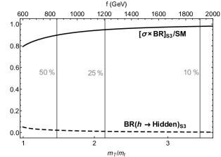
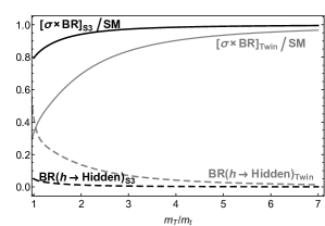
Figure 6: (Left) Plot of the signal strength of producing $h$ and it directly decaying to SM particles and the branching ratio for decays $h$ decays to A and B sector particles. The plot is given as a function of both the order breaking parameter $f$ and the ratio of the top partner masses divided by the SM top mass. (Right) Comparison plot of the signal strength and branching fraction of hidden sector $h$ decays plotted as a function of the top partner mass ratios.

As mentioned in Section 5 in order to associate the $A$-sector with the SM-like sector we needed to tune $\frac{\rho^{2}}{\delta}$ against $\frac{m^{2}}{6\lambda+\delta}$ which resulted in a modest tuning of order $6v^{2}/f^{2}$. A tree level tuning of 50%, 25%, and 10% corresponds to an $SU(12)$ breaking order parameter of $f\approx$ 0.85 TeV, 1.2 TeV, and 1.9 TeV respectively, or equivalently in terms of the top partner mass of $m_{T}\approx$ 1.48$m_{t}$, 2.14$m_{t}$, and 3.43 $m_{t}$. We overlay the plot in Figure 6 with lines indicating these tree level tunings.

6 Results and Future Prospects

The $S_{3}$-orbifold Higgs can easily accommodate the SM without facing any major tuning for cutoff scales approaching $8$ TeV. A 10% tree level tuning is sufficient to give the signal strength the SM Higgs within a couple percent. Though the nature of the model may seem complicated with three sectors which can only communicate through the Higgs portal, the Higgs phenomenology is only dependent on two additional parameter to the SM, the $SU(12)$ breaking order parameter $f$ and the soft term $\rho$. This makes the testability of model in principle no more complicated than Twin Higgs.

The LHC has greater sensitivity in measuring signals from SM decays of the Higgs compared to invisible decays. This makes searching for deviations in SM Higgs decay channels favorable for testing the model. At an integrated luminosity of $3000\mbox{ fb}^{-1}$ the LHC will be able to probe Higgs signal strengths in the $WW$, $ZZ$, and $\gamma\gamma$ channels down to the 5% level[27]. If a suppression in the signal strengths of more than 5% is measured, the model will be pushed into the region of parameter space where with top partner masses $m_{T}\lesssim 2m_{t}$. This makes it difficult for the LHC to strongly disfavor the $S_{3}$-orbifold Higgs as a natural model. The increased Higgs production of a 100 TeV collider however may provide a way of testing the naturalness of the model.

There is also the possibility for more exotic collider signatures in the form of Higgs decays with displaced vertices. It is possible for the SM-like Higgs to decay into $B$ and $C$-sector states which may decay back into SM states giving rise to so-called “hidden valley” signatures[28, 29, 30]. These signatures were studied in the context of the Fraternal Twin Higgs[31]. The phenomenology in the $S_{3}$-orbifold Higgs model should be qualitatively similar. A thorough comparison would require a more detailed study of the hidden sectors and mass scales of the glueballs produced in each sector, including those that may be produced by the unbroken $SU(3)$ subgroup of the broken $SU(4)$ weak gauge group in the $C$-sector.

An interesting feature of the model is that for relatively light top partners, in comparison to those in the Twin Higgs, there is still a large suppression of Higgs decays to hidden sector states. This is a general feature of orbifold Higgs models where the orbifold projection produces three or more sectors. With such a modest difference in the masses of fermion partners it may be interesting to study if any of the matter in the hidden sectors could serve as a stable dark matter candidate. The possibility of $C-$sector having multiple confining gauge groups in the theory may also provide additional stability against the states decaying into SM states. There have already been a number of dark matter and cosmology studies involving the Twin Higgs[34, 33, 32, 35, 36, 37, 38, 39, 40, 41] which may serve as an avenue for future work involving the $S_{3}$-orbifold Higgs model.

7 Acknowledgments

Many thanks to Marc Sher, Christopher Carone, and Joshua Erlich for thoughtful discussions. This work was supported by the NSF under Grant PHY-1519644.

Appendix A Appendix

Scalar multiplets of the daughter theory in the Hermitian basis.

$$\begin{array}[]{ccc}h_{A}=\frac{1}{\sqrt{2}}\left(\begin{array}[]{c}\phi_{A}^{1}+i\phi_{A}^{2}\\ (v_{A}+\phi_{A}^{3})+i\phi_{A}^{4}\end{array}\right)&&h_{B}=\frac{1}{\sqrt{2}}\left(\begin{array}[]{c}\phi_{B}^{1}+i\phi_{B}^{2}\\ (v_{B}+\phi_{B}^{3})+i\phi_{B}^{4}\end{array}\right)\\ &&\\ h_{C_{1}}=\frac{1}{\sqrt{2}}\left(\begin{array}[]{c}\phi_{C_{1}}^{1}+i\phi_{C_{1}}^{2}\\ \phi_{C_{1}}^{3}+i\phi_{C_{1}}^{4}\\ \phi_{C_{1}}^{5}+i\phi_{C_{1}}^{6}\\ (v_{C_{1}}+\phi_{C_{1}}^{7})+i\phi_{C_{1}}^{8}\end{array}\right)&&h_{C_{2}}=\frac{1}{\sqrt{2}}\left(\begin{array}[]{c}\phi_{C_{2}}^{1}+i\phi_{C_{2}}^{2}\\ \phi_{C_{2}}^{3}+i\phi_{C_{2}}^{4}\\ \phi_{C_{2}}^{5}+i\phi_{C_{2}}^{6}\\ (v_{C_{2}}+\phi_{C_{2}}^{7})+i\phi_{C_{2}}^{8}\end{array}\right)\end{array}$$ (A.1)

The scalar mass eigenstates given in terms of the fields of the Hermitian basis with $\theta=v/f$ and $c_{\theta}\equiv\cos\theta$ $s_{\theta}\equiv\sin\theta$.

$$\left(\begin{array}[]{c}h\\ H_{1}\\ H_{2}\\ H_{radial}\end{array}\right)=\left(\begin{array}[]{cccc}c_{\theta}&-\frac{1}{\sqrt{5}}s_{\theta}&-\frac{\sqrt{2}}{\sqrt{5}}s_{\theta}&-\frac{\sqrt{2}}{\sqrt{5}}s_{\theta}\\ 0&\frac{2}{\sqrt{5}}&\frac{-1}{\sqrt{10}}&\frac{-1}{\sqrt{10}}\\ 0&0&\frac{1}{\sqrt{2}}&\frac{-1}{\sqrt{2}}\\ s_{\theta}&\frac{1}{\sqrt{5}}c_{\theta}&\frac{\sqrt{2}}{\sqrt{5}}c_{\theta}&\frac{\sqrt{2}}{\sqrt{5}}c_{\theta}\end{array}\right)\left(\begin{array}[]{c}\phi_{A}^{3}\\ \phi_{B}^{3}\\ \phi_{C_{1}}^{7}\\ \phi_{C_{2}}^{7}\end{array}\right)$$ (A.2)

$$\begin{array}[]{ccc}H_{3}=\frac{1}{\sqrt{2}}\left(\phi_{C_{1}}^{1}-\phi_{C_{2}}^{1}\right)&H_{4}=\frac{1}{\sqrt{2}}\left(\phi_{C_{1}}^{2}-\phi_{C_{2}}^{2}\right)&H_{5}=\frac{1}{\sqrt{2}}\left(\phi_{C_{1}}^{3}-\phi_{C_{2}}^{3}\right)\\ H_{6}=\frac{1}{\sqrt{2}}\left(\phi_{C_{1}}^{4}-\phi_{C_{2}}^{4}\right)&H_{7}=\frac{1}{\sqrt{2}}\left(\phi_{C_{1}}^{5}-\phi_{C_{2}}^{5}\right)&H_{8}=\frac{1}{\sqrt{2}}\left(\phi_{C_{1}}^{6}-\phi_{C_{2}}^{6}\right)\\ &H_{9}=\frac{1}{\sqrt{2}}\left(\phi_{C_{1}}^{8}-\phi_{C_{2}}^{8}\right)&\end{array}$$ (A.3)

Below we list the corresponding masses for the mass eigenstate given above.

$$m^{2}_{H_{1}} \approx \frac{2}{5}\delta f^{2}\cos^{2}\left(\frac{v}{f}\right)$$ (A.4)

$$m^{2}_{H_{2}} \approx \frac{2}{5}\delta f^{2}\cos^{2}\left(\frac{v}{f}\right)+2\sigma^{2}$$ (A.5)

$$m^{2}_{H_{3-9}} \approx 2\sigma^{2}$$ (A.6)

$$m^{2}_{H_{radial}} \approx 2\lambda f^{2}$$ (A.7)

Functions appearing in the Higgs partial decay widths.

$$A_{V}(x) = -x^{2}\left[\frac{2}{x^{2}}+\frac{3}{x}+3\left(\frac{2}{x}-1\right)\arcsin^{2}\left(\frac{1}{\sqrt{x}}\right)\right]$$ (A.8)

$$A_{F}(x) = 2x^{2}\left[\frac{1}{x}+\left(\frac{1}{x}-1\right)\arcsin^{2}\left(\frac{1}{\sqrt{x}}\right)\right]$$ (A.9)

$$\delta_{W} = 1$$ (A.10)

$$\delta_{Z} = \frac{7}{12}-\frac{10}{9}\sin^{2}\theta_{W}+\frac{40}{9}\sin^{4}\theta_{W}$$ (A.11)

$$R_{T}(x)= \frac{3(1-8x+20x^{2})}{\sqrt{4x-1}}\cos^{-1}\left(\frac{3x-1}{2x^{3/2}}\right)-\frac{1-x}{2x}(2-13x+47x^{2})$$

$$-\frac{3}{2}(1-6x+4x^{2})\ln x\,$$ (A.12)

References

- [1] ATLAS Collaboration Collaboration, G. Aad et al., Observation of a new particle in the search for the Standard Model Higgs boson with the ATLAS detector at the LHC, Phys.Lett. B716 (2012) 1–29, [arXiv:1207.7214].
- [2] CMS Collaboration Collaboration, S. Chatrchyan et al., Observation of a new boson at a mass of 125 GeV with the CMS experiment at the LHC, Phys.Lett. B716 (2012) 30–61, [arXiv:1207.7235].
- [3] R. Barbieri and A. Strumia, hep-ph/0007265.
- [4] Z. Chacko, H. S. Goh and R. Harnik, “The Twin Higgs: Natural electroweak breaking from mirror symmetry,” Phys. Rev. Lett. 96, 231802 (2006) doi:10.1103/PhysRevLett.96.231802 [hep-ph/0506256].
- [5] Z. Chacko, H. S. Goh and R. Harnik, JHEP 0601, 108 (2006) doi:10.1088/1126-6708/2006/01/108 [hep-ph/0512088].
- [6] P. Batra and Z. Chacko, A Composite Twin Higgs Model, Phys.Rev. D79 (2009) 095012, arXiv:0811.0394 [hep-ph].
- [7] R. Barbieri, D. Greco, R. Rattazzi, and A. Wulzer, The Composite Twin Higgs scenario, arXiv:1501.07803 [hep-ph].
- [8] M. Low, A. Tesi, and L.-T. Wang, Twin Higgs mechanism and a composite Higgs boson, Phys.Rev. D91 (2015) no. 9, 095012, arXiv:1501.07890 [hep-ph].
- [9] M. Badziak and K. Harigaya, arXiv:1703.02122 [hep-ph].
- [10] A. Katz, A. Mariotti, S. Pokorski, D. Redigolo and R. Ziegler, JHEP 1701, 142 (2017) doi:10.1007/JHEP01(2017)142 [arXiv:1611.08615 [hep-ph]].
- [11] M. Geller and O. Telem, A Holographic Twin Higgs Model, Phys.Rev.Lett. 114 (2015) no. 19, 191801, arXiv:1411.2974 [hep-ph].
- [12] N. Craig and K. Howe, Doubling down on naturalness with a supersymmetric twin Higgs, JHEP 1403 (2014) 140, arXiv:1312.1341 [hep-ph].
- [13] A. Falkowski, S. Pokorski and M. Schmaltz, Phys. Rev. D 74, 035003 (2006) doi:10.1103/PhysRevD.74.035003 [hep-ph/0604066].
- [14] S. Chang, L. J. Hall, and N. Weiner, A Supersymmetric twin Higgs, Phys. Rev. D75 (2007) 035009, arXiv:hep-ph/0604076 [hep-ph].
- [15] G. Burdman, Z. Chacko, H. S. Goh and R. Harnik, JHEP 0702, 009 (2007) doi:10.1088/1126-6708/2007/02/009 [hep-ph/0609152].
- [16] H. Cai, H. C. Cheng and J. Terning, JHEP 0905, 045 (2009) doi:10.1088/1126-6708/2009/05/045 [arXiv:0812.0843 [hep-ph]].
- [17] Z. Chacko, Y. Nomura, M. Papucci and G. Perez, JHEP 0601, 126 (2006) doi:10.1088/1126-6708/2006/01/126 [hep-ph/0510273].
- [18] B. Batell and M. McCullough, Phys. Rev. D 92, no. 7, 073018 (2015) doi:10.1103/PhysRevD.92.073018 [arXiv:1504.04016 [hep-ph]].
- [19] N. Arkani-Hamed, T. Cohen, R. T. D’Agnolo, A. Hook, H. D. Kim and D. Pinner, Phys. Rev. Lett. 117, no. 25, 251801 (2016) doi:10.1103/PhysRevLett.117.251801 [arXiv:1607.06821 [hep-ph]].
- [20] N. Craig, S. Knapen and P. Longhi, Phys. Rev. Lett. 114 (2015) no.6, 061803 doi:10.1103/PhysRevLett.114.061803 [arXiv:1410.6808 [hep-ph]].
- [21] N. Craig, S. Knapen and P. Longhi, JHEP 1503, 106 (2015) doi:10.1007/JHEP03(2015)106 [arXiv:1411.7393 [hep-ph]].
- [22] M. Schmaltz, Phys. Rev. D 59, 105018 (1999) doi:10.1103/PhysRevD.59.105018 [hep-th/9805218].
- [23] E. C. G. Stueckelberg, Helv. Phys. Acta 11, 225 (1938). doi:10.5169/seals-110852
- [24] H. Ruegg and M. Ruiz-Altaba, Int. J. Mod. Phys. A 19, 3265 (2004) doi:10.1142/S0217751X04019755 [hep-th/0304245].
- [25] G. Burdman, Z. Chacko, R. Harnik, L. de Lima and C. B. Verhaaren, Phys. Rev. D 91, no. 5, 055007 (2015) doi:10.1103/PhysRevD.91.055007 [arXiv:1411.3310 [hep-ph]].
- [26] A. Djouadi, Phys. Rept. 457, 1 (2008) doi:10.1016/j.physrep.2007.10.004 [hep-ph/0503172].
- [27] S. Dawson et al., arXiv:1310.8361 [hep-ex].
- [28] M. J. Strassler and K. M. Zurek, Phys. Lett. B 651, 374 (2007) doi:10.1016/j.physletb.2007.06.055 [hep-ph/0604261].
- [29] M. J. Strassler and K. M. Zurek, Phys. Lett. B 661, 263 (2008) doi:10.1016/j.physletb.2008.02.008 [hep-ph/0605193].
- [30] T. Han, Z. Si, K. M. Zurek and M. J. Strassler, JHEP 0807, 008 (2008) doi:10.1088/1126-6708/2008/07/008 [arXiv:0712.2041 [hep-ph]].
- [31] N. Craig, A. Katz, M. Strassler and R. Sundrum, JHEP 1507, 105 (2015) doi:10.1007/JHEP07(2015)105 [arXiv:1501.05310 [hep-ph]].
- [32] R. Barbieri, L. J. Hall and K. Harigaya, JHEP 1611, 172 (2016) doi:10.1007/JHEP11(2016)172 [arXiv:1609.05589 [hep-ph]].
- [33] Z. Chacko, N. Craig, P. J. Fox and R. Harnik, [arXiv:1611.07975 [hep-ph]].
- [34] N. Craig, S. Koren and T. Trott, arXiv:1611.07977 [hep-ph].
- [35] V. Prilepina and Y. Tsai, arXiv:1611.05879 [hep-ph].
- [36] M. Farina, JCAP 1511, no. 11, 017 (2015) doi:10.1088/1475-7516/2015/11/017 [arXiv:1506.03520 [hep-ph]].
- [37] M. Farina, A. Monteux and C. S. Shin, Phys. Rev. D 94, no. 3, 035017 (2016) doi:10.1103/PhysRevD.94.035017 [arXiv:1604.08211 [hep-ph]].
- [38] I. Garcia Garcia, R. Lasenby and J. March-Russell, Phys. Rev. Lett. 115, no. 12, 121801 (2015) doi:10.1103/PhysRevLett.115.121801 [arXiv:1505.07410 [hep-ph]].
- [39] N. Craig and A. Katz, JCAP 1510, no. 10, 054 (2015) doi:10.1088/1475-7516/2015/10/054 [arXiv:1505.07113 [hep-ph]].
- [40] I. Garcia Garcia, R. Lasenby and J. March-Russell, Phys. Rev. D 92, no. 5, 055034 (2015) doi:10.1103/PhysRevD.92.055034 [arXiv:1505.07109 [hep-ph]].
- [41] C. Csaki, E. Kuflik and S. Lombardo, arXiv:1703.06884 [hep-ph].