Emergence of spacetime discreteness in Wightman function from polymer quantization of scalar field

Abstract

The Wightman function i.e. vacuum two-point function, for a massless free scalar field in Fock quantization is inversely proportional to the invariant distance squared between the corresponding spacetime points. Naturally it diverges when these two points are taken to be infinitesimally close to each other. Using a combination of analytical and numerical methods, we show that the Wightman function is bounded from above in polymer quantization of scalar field. The bounded value of the Wightman function is governed by the polymer scale and its bounded nature can be viewed as if the spacetime has a zero-point length. This emergence of effective discreteness in spacetime appears from polymer quantization of matter field alone as the geometry is treated classically. It also demonstrates that the polymer quantization of matter field itself can capture certain aspects of the effective discrete geometry. We discuss the implications of the result on the response function of a Unruh-DeWitt detector that depends on the properties of the Wightman function.

I Introduction

The vacuum two-point function which is usually known as the Wightman function Peskin and Schroeder (1995); Kaku (1993); Birrell and Davies (1984); Ford (1997), plays an important role in disseminating the implications of the quantum field theory. As an example, it is often employed to see whether the causality is preserved by the field in a given quantum field theory. In addition, the Wightman function has been used as a probe to understand the structure of the underlying spacetime Blau et al. (2010); Kapustin (2001); Mercuri (2009); Raasakka (2017). One way to visualize this aspect is to note that the Wightman function for a massless free scalar field in Fock quantization is inversely proportional to the invariant distance squared between the corresponding spacetime points. This relation then may be used in reverse to conclude about the nature of the effective spacetime distance between two given points, as experienced by the field, if one knows the corresponding Wightman function. Therefore, if one computes the Wightman function in a theory which aims to modify physics near Planck scale then one could use it to see whether the properties of such a Wightman function indicate any Plank scale alteration to the effective spacetime distance. For example, one could ask whether the notion of zero-point length can emerge from the properties of the Wightman function.

Besides, the Wightman function is also known to play an important role in realizing aspects of certain quantum phenomena in curved spacetime such as the Unruh effect Birrell and Davies (1984); Crispino et al. (2008); Takagi (1986); Unruh (1976). In particular, the response function of a Unruh-Dewitt detector depends on the structure of the pole of the Wightman function. In the context of polymer quantization, it has been argued that Unruh effect could disappear Hossain and Sardar (2016a); Hossain and Sardar (2015); Hossain and Sardar (2016b) due to the presence of a new length scale. The polymer quantization Ashtekar et al. (2003); Halvorson (2004) is a canonical quantization method which is used in Loop Quantum gravity Ashtekar and Lewandowski (2004); Rovelli (2004); Thiemann (2007). Some key aspects of polymer quantization are known to differ from Schrodinger quantization when one applies it to a mechanical system. Consequently, in polymer quantization of the field one expects to find some results which are different from the Fock quantization. Therefore, it is imperative to study the properties of the Wightman function in the context of polymer quantization and some qualitative aspects of it are already noted in Hossain and Sardar (2015); Hossain and Sardar (2016b). A complete analytical computation of the Wightman function in polymer quantization turns out to be very difficult. Therefore, in order to understand the behaviour of the Wightman function for a wide range of spacetime intervals, in this article we employ a combination of both analytical and numerical techniques in the context of polymer quantization of scalar matter field in a classical flat geometry.

This paper is organized as follows. In the section II, we consider a massless free scalar field in the canonical framework. Subsequently, we review the general derivation of the Wightman function in the canonical approach and derive the same for Fock quantization in the section III. In the section IV, we briefly discuss some key results from polymer quantization which are relevant for computation of the Wightman function. Then, we analytically compute the Wightman function in the asymptotic regions for the timelike and the spacelike intervals separately. Subsequently, we employ numerical techniques to compute it for a wide range of spacetime intervals. Using both analytical and numerical computations, we show that unlike in Fock quantization, the Wightman function is bounded from above in polymer quantization. Its bounded nature is governed by the new polymer length scale and this property can be viewed as if the spacetime has a notion of zero-point length.

II Massless scalar field

In order to study the properties of the two-point function, we consider here a massless free scalar field $\Phi(x)$ in Minkowski spacetime. The dynamics of such a scalar field is described by the action

$$S_{\Phi}=\int d^{4}x\left[-\frac{1}{2}\sqrt{-\eta}\eta^{\mu\nu}\partial_{\mu}\Phi(x)\partial_{\nu}\Phi(x)\right]~{},$$ (1)

where the invariant distance element can be expressed as

$$ds^{2}=\eta_{\mu\nu}dx^{\mu}dx^{\nu}=-dt^{2}+q_{ab}d\mathbf{x}^{a}d\mathbf{x}^{b}~{}.$$ (2)

Here we use the natural units $c=\hbar=1$ and the metric is $\eta_{\mu\nu}=diag(-1,1,1,1)$. In this article, for quantization of the matter field, we aim to apply polymer quantization method which is a canonical approach. Therefore, we need to compute the Hamiltonian associated with the scalar field action (1). By choosing spatial hyper-surfaces, each of which is labeled by given time $t$, one can express the corresponding scalar field Hamiltonian as

$$H_{\Phi}=\int d^{3}\mathbf{x}\left[\frac{\Pi^{2}}{2\sqrt{q}}+\frac{\sqrt{q}}{2}q^{ab}\partial_{a}\Phi\partial_{b}\Phi\right]~{},$$ (3)

where $q_{ab}$ is the spatial metric and $q$ is its determinant. The Poisson bracket between the field $\Phi=\Phi(t,\mathbf{x})$ and the conjugate field momentum $\Pi=\Pi(t,\mathbf{x})$ is given by

$$\{\Phi(t,\mathbf{x}),\Pi(t,\mathbf{y})\}=\delta^{3}(\mathbf{x}-\mathbf{y})~{}.$$ (4)

II.1 Fourier modes

In this article we follow the polymer quantization approach as suggested in Hossain et al. (2010) where one performs explicit Fourier transformation of the field to express it as a set of decoupled simple harmonic oscillators before quantization. In particular, one defines the Fourier modes for the scalar field and its conjugate momentum as

$$\Phi=\frac{1}{\sqrt{V}}\sum_{\mathrm{k}}\tilde{\phi}_{\mathrm{k}}(t)e^{i\mathrm{k}\cdot\mathbf{x}},~{}\Pi=\frac{1}{\sqrt{V}}\sum_{\mathrm{k}}\sqrt{q}~{}\tilde{\pi}_{\mathrm{k}}(t)e^{i\mathrm{k}\cdot\mathbf{x}},$$ (5)

where $V=\int d^{3}\mathbf{x}\sqrt{q}$ is the spatial volume. In Minkowski spacetime, due to the non-compactness of the spatial hyper-surfaces, the spatial volume will diverge. Therefore, using a fiducial box of finite volume, one can avoid to have such a divergent quantity in the intermediate steps. In such case, Kronecker delta and Dirac delta are expressed as $\int d^{3}\mathbf{x}\sqrt{q}~{}e^{i(\mathrm{k}-\mathrm{k}^{\prime})\cdot\mathbf{x}}=V\delta_{\mathrm{k},\mathrm{k}^{\prime}}$ and $\sum_{\mathrm{k}}e^{i\mathrm{k}\cdot(\mathbf{x}-\mathbf{y})}=V\delta^{3}(\mathbf{x}-\mathbf{y})/\sqrt{q}$.

II.2 Hamiltonian density of the modes

Using the expressions of Kronecker delta and Dirac delta, the Hamiltonian (3) can be expressed fully in terms of Fourier modes (5). In particular, the field Hamiltonian (3) can be expressed as $H_{\Phi}=\sum_{\mathrm{k}}\mathcal{H}_{\mathrm{k}}$, where the Hamiltonian density for the $\mathrm{k}^{th}$ mode is

$$\mathcal{H}_{\mathrm{k}}=\frac{1}{2}\tilde{\pi}_{-\mathrm{k}}\tilde{\pi}_{\mathrm{k}}+\frac{1}{2}|\mathrm{k}|^{2}\tilde{\phi}_{-\mathrm{k}}\tilde{\phi}_{\mathrm{k}}~{}.$$ (6)

The non-vanishing Poisson brackets between the modes are given by

$$\{\tilde{\phi}_{\mathrm{k}},\tilde{\pi}_{-\mathrm{k}^{\prime}}\}=\delta_{\mathrm{k},\mathrm{k}^{\prime}}~{}.$$ (7)

The Fourier modes of field $\tilde{\phi}_{\mathrm{k}}$ and its conjugate momenta $\tilde{\pi}_{\mathrm{k}}$ are in general complex-valued functions. Therefore, each complex-valued mode has two independent real-valued modes. For a real-valued scalar field $\Phi$, one can impose a reality condition to redefine the complex-valued modes $\tilde{\phi}_{\mathrm{k}}$ and $\tilde{\pi}_{\mathrm{k}}$ in terms of the real-valued modes, say, $\phi_{\mathrm{k}}$ and $\pi_{\mathrm{k}}$ respectively. In terms of these real-valued mode functions, the corresponding Hamiltonian density and the Poisson brackets can be expressed as

$$\mathcal{H}_{\mathrm{k}}=\frac{1}{2}\pi_{\mathrm{k}}^{2}+\frac{1}{2}|\mathrm{k}|^{2}\phi_{\mathrm{k}}^{2}~{}~{}~{};~{}~{}~{}\{\phi_{\mathrm{k}},\pi_{\mathrm{k}^{\prime}}\}=\delta_{\mathrm{k},\mathrm{k}^{\prime}}~{}.$$ (8)

The equation (8) represents a standard system of decoupled harmonic oscillators. Clearly, a free scalar field can be viewed as a composition of infinitely many decoupled harmonic oscillators.

II.3 General form of Wightman function

The standard Fock quantization of the scalar field is achieved by quantizing these simple harmonic oscillators using Schrodinger quantization as if each of these modes were a mechanical system. Analogously, we shall use the polymer quantization for these modes in order to perform polymer quantization of the scalar field.

In general, we may express the energy spectrum of these quantum oscillators as $\hat{\mathcal{H}}_{\mathrm{k}}|n_{\mathrm{k}}\rangle=E_{n}^{(\mathrm{k})}|n_{\mathrm{k}}\rangle$ where the energy eigenvalues $E_{n}^{(\mathrm{k})}$ of the $\mathrm{k}^{th}$ oscillator corresponds to the energy eigenstates $|n_{\mathrm{k}}\rangle$. The corresponding vacuum state for the field can then be expressed as $|0\rangle=\Pi_{\mathrm{k}}\otimes|0_{\mathrm{k}}\rangle$. Therefore, the general form of the vacuum two-point function which is also known as the Wightman function, can be expressed as

$$G(x,x^{\prime})\equiv\langle 0|\hat{\Phi}(x)\hat{\Phi}(x^{\prime})|0\rangle=\langle 0|\hat{\Phi}(t,\mathbf{x})\hat{\Phi}(t^{\prime},\mathbf{x}^{\prime})|0\rangle~{}.$$ (9)

In terms of the Fourier modes (5), one can express the Wightman function (9) as

$$G(x,x^{\prime})=\frac{1}{V}\sum_{\mathrm{k}}D_{\mathrm{k}}(t,t^{\prime})~{}e^{i{\mathrm{k}}\cdot(\mathbf{x}-\mathbf{x}^{\prime})},$$ (10)

where the matrix element can be written as

$$D_{\mathrm{k}}(t,t^{\prime})=\langle 0_{\mathrm{k}}|e^{i\hat{\mathcal{H}}_{\mathrm{k}}t}\hat{\phi}_{\mathrm{k}}e^{-i\hat{\mathcal{H}}_{\mathrm{k}}t}e^{i\hat{\mathcal{H}}_{\mathrm{k}}t^{\prime}}\hat{\phi}_{\mathrm{k}}e^{-i\hat{\mathcal{H}}_{\mathrm{k}}t^{\prime}}|0_{\mathrm{k}}\rangle.$$ (11)

We may expand the state $\hat{\phi}_{\mathrm{k}}|0_{\mathrm{k}}\rangle$ in the complete basis of the energy eigenstates as $\hat{\phi}_{\mathrm{k}}|0_{\mathrm{k}}\rangle=\sum_{n}c_{n}|n_{\mathrm{k}}\rangle$. Subsequently, by using the energy spectrum, we can express the matrix element as

$$D_{\mathrm{k}}(t-t^{\prime})\equiv D_{\mathrm{k}}(t,t^{\prime})=\sum_{n}|c_{n}|^{2}e^{-i\Delta E_{n}(t-t^{\prime})},$$ (12)

where the energy gaps $\Delta E_{n}\equiv E_{n}^{(\mathrm{k})}-E_{0}^{(\mathrm{k})}$ and the coefficients $c_{n}=\langle n_{\mathrm{k}}|\hat{\phi}_{\mathrm{k}}|0_{\mathrm{k}}\rangle$.

Thanks to the chosen definition of Fourier modes (5), the Hamiltonian density and Poisson brackets of the modes are already independent of the fiducial volume. The remaining fiducial volume dependence in the expression of the Wightman function (10) can be removed by taking the limit $V\to\infty$ such that the summation becomes an integral. In other words, we can remove the fiducial volume, by essentially replacing the sum $\frac{1}{V}\sum_{\mathrm{k}}$ by an integration $\int\frac{d^{3}\mathrm{k}}{(2\pi)^{3}}$. The Wightman function (10) then becomes

$$G(x,x^{\prime})=\int\frac{d^{3}\mathrm{k}}{(2\pi)^{3}}~{}D_{\mathrm{k}}(t,t^{\prime})~{}e^{i{\mathrm{k}}\cdot(\mathbf{x}-\mathbf{x}^{\prime})}~{}.$$ (13)

The matrix element of $D_{\mathrm{k}}(t-t^{\prime})$ depends on $\mathrm{k}$ through its magnitude for both Fock quantization and the polymer quantization. Therefore, in order to evaluate the integration (13), we use polar coordinates in momentum space as following

$$G(x,x^{\prime})=\int\frac{k^{2}dk}{4\pi^{2}}D_{k}(\Delta t)\int\sin\theta d\theta~{}e^{ik|\Delta\mathbf{x}|\cos\theta},$$ (14)

where $k=|\mathrm{k}|$, $\Delta\mathbf{x}=\mathbf{x}-\mathbf{x}^{\prime}$ and $\Delta t=t-t^{\prime}$. By performing the integration over the angle $\theta$, one can express the Wightman function as

$$G(x,x^{\prime})=G_{+}-G_{-}~{},$$ (15)

where

$$G_{\pm}=\frac{i}{4\pi^{2}|\Delta\mathbf{x}|}\int dk~{}kD_{k}(\Delta t)~{}e^{\mp ik|\Delta\mathbf{x}|}~{}.$$ (16)

Using the equations (15) and (16), we note that the Wightman function depends only on the magnitude of the spatial separation $\Delta\mathbf{x}$. On the other hand it is sensitive also to the sign of the temporal separation $\Delta t$. An important consequence of these dependences is that the vacuum expectation value of the commutator bracket $\langle 0|[\hat{\Phi}(x),\hat{\Phi}(x^{\prime})]|0\rangle=G(x,x^{\prime})-G(x^{\prime},x)=0$ when temporal separation $\Delta t=0$ for the given two spacetime points $x$, $x^{\prime}$. For a spacelike separation in Minkowski spacetime, one can always choose a frame where the temporal separation $\Delta t$ vanishes. These aspects together imply that no causal communication is possible between any two spacelike events.

In general, the integrals in the equation (16) are not convergent. Therefore, one needs to employ some form of regularization techniques to render them finite. Here we use the standard prescription where one introduces a non-oscillatory regulator term in the integral as follows

$$G_{\pm}^{\delta}=\frac{i}{4\pi^{2}|\Delta\mathbf{x}|}\int dk~{}kD_{k}(\Delta t)~{}e^{\mp ik|\Delta\mathbf{x}|}~{}e^{-\delta~{}k}~{}.$$ (17)

Here $\delta$ is taken to be a positive parameter such that $\lim_{\delta\to 0}G_{\pm}^{\delta}=G_{\pm}$.

III Fock quantization

As we have mentioned earlier that the Fock quantization is achieved by quantizing the modes (8) using Schrodinger quantization. In particular, there one seeks to represent the elementary commutator bracket $\left[\hat{\phi}_{\mathrm{k}},\hat{\pi}_{\mathrm{k}}\right]=i$ for the given mode on the Hilbert space. It is then straightforward to compute the energy spectrum for the $\mathrm{k}^{th}$ mode which is given by $E_{n}^{(\mathrm{k})}=(n+\frac{1}{2})|\mathrm{k}|$. The corresponding coefficients are $c_{n}=\delta_{1,n}/\sqrt{2|\mathrm{k}|}$ and the energy gaps are $\Delta E_{n}=n|\mathrm{k}|$. The Wightman function (15) for the Fock quantization then becomes

$$G^{\delta}(x,x^{\prime})=\frac{1}{4\pi^{2}\left[-(\Delta t-i\delta)^{2}+|\Delta\mathbf{x}|^{2}\right]}~{},$$ (18)

where the parameter $\delta$ is introduced as the regulator of the integral. If we remove the regulator by taking the limit $\delta\to 0$ then the Wightman function (18) becomes

$$G(x,x^{\prime})=\frac{1}{4\pi^{2}\Delta x^{2}}~{},$$ (19)

where $\Delta x^{2}=-\Delta t^{2}+|\Delta\mathbf{x}|^{2}$ is the usual invariant distance interval in the Minkowski spacetime.

IV Polymer quantization

We now briefly review some relevant results from polymer quantization for the computation of the Wightman function. The polymer quantization is a canonical quantization method which is used in loop quantum gravity. Apart from the Planck constant $\hbar$, it comes with a new dimension-full parameter, say $l_{\star}$. In full quantum gravity, this length scale would correspond to the Planck length. However, in this article we treat the background geometry as classical and we apply polymer quantization only for the matter field.

In polymer quantization it is shown that the exact energy spectrum of the $\mathrm{k}^{th}$ harmonic oscillator can be expressed in terms of the Mathieu characteristic value functions $A_{n}$, $B_{n}$ as Hossain et al. (2010)

$$\frac{E_{\mathrm{k}}^{2n}}{|\mathrm{k}|}=\frac{1}{4g}+\frac{g}{2}~{}A_{n}(g)~{},~{}\frac{E_{\mathrm{k}}^{2n+1}}{|\mathrm{k}|}=\frac{1}{4g}+\frac{g}{2}B_{n+1}(g)~{},$$ (20)

where $n\geq 0$ and $g=|\mathrm{k}|~{}l_{\star}$ is a dimension-less parameter. The corresponding energy eigenstates are $\psi_{2n}(v)=\mathrm{ce}_{n}(1/4g^{2},v)/\sqrt{\pi}$ and $\psi_{2n+1}(v)=\mathrm{se}_{n+1}(1/4g^{2},v)/\sqrt{\pi}$ where $v=\pi_{\mathrm{k}}\sqrt{l_{\star}}+\pi/2$. These functions $\mathrm{ce}_{n}$ and $\mathrm{se}_{n}$ are solutions to Mathieu equations which are known as elliptic cosine and sine functions respectively Abramowitz and Stegun (1964). We should mention here that the superselection rules are employed to arrive at these $\pi$-periodic and $\pi$-antiperiodic states in $v$. Without imposition of any such superselection rules, some statistical features of the system are known to be ill-defined Barbero G. et al. (2013).

In polymer quantization, the coefficients $c_{4n+3}=i\sqrt{l_{\star}}\int_{0}^{2\pi}\psi_{4n+3}\partial_{v}\psi_{0}dv$ are non-vanishing for all positive integer $n$ whereas in Fock quantization only one $c_{n}$ is non-vanishing. Using the asymptotic expressions of $A_{n}$ and $B_{n}$, it is shown that the energy spectrum (20) reduces to regular harmonic oscillator energy spectrum along with perturbative corrections in the small $g$ limit Hossain et al. (2010). In particular, the relevant energy gaps for sub-Planckian modes (i.e. $g\ll 1$) can be expressed as

$$\frac{\Delta E_{4n+3}}{|\mathrm{k}|}=(2n+1)-\frac{(4n+3)^{2}-1}{16}g+\mathcal{O}\left(g^{2}\right)~{},$$ (21)

for $n\geq 0$. On the other hand, for super-Planckian modes (i.e. $g\gg 1$), one can approximate the energy gaps as

$$\frac{\Delta E_{4n+3}}{|\mathrm{k}|}=2(n+1)^{2}g+\mathcal{O}\left(\frac{1}{g^{3}}\right),$$ (22)

for $n\geq 0$. One may note that the form of the energy gaps (22) for super-Planckian modes significantly differ from the corresponding energy gaps obtained from Fock quantization.

Using asymptotic behavior of the Mathieu functions in small $g$ limit, one can approximate the coefficients as

$$c_{3}=\frac{i}{\sqrt{2|\mathrm{k}|}}\left[1+\mathcal{O}\left(g\right)\right]~{},~{}\frac{c_{4n+3}}{c_{3}}=\mathcal{O}\left(g^{n}\right),$$ (23)

where $n>0$. On the other hand, for the limit $g\gg 1$, the coefficients can be expressed as

$$c_{3}=i\sqrt{\frac{g}{2|\mathrm{k}|}}\left[\frac{1}{4g^{2}}+\mathcal{O}\left(\frac{1}{g^{6}}\right)\right],\frac{c_{4n+3}}{c_{3}}=\mathcal{O}\left(\frac{1}{g^{2n}}\right),$$ (24)

for $n>0$. Using the equations (23) and (24), it is clear that in polymer quantization one can approximate the matrix elements as

$$D_{\mathrm{k}}(\Delta t)\simeq|c_{3}|^{2}e^{-i\Delta E_{3}\Delta t}\equiv|c_{k}|^{2}e^{-i\Delta E_{k}\Delta t}~{},$$ (25)

for both asymptotic regions.

IV.1 Sub-Planckian and super-Planckian contributions to Wightman function

Unlike in the case of Fock quantization, the exact analytical computation of the Wightman function for all possible spacetime intervals does not seem to be possible in polymer quantization. However, it is possible to perform analytic computation for asymptotic regions and some qualitative aspects of it has already been noted in Hossain and Sardar (2015); Hossain and Sardar (2016b). Asymptotic expressions of the Wightman function also becomes very useful for checking the consistency of its numerically evaluated values.

From the equations (16) and (25), we note that the expression of the Wightman function is determined by the expressions of $|c_{k}|^{2}\equiv|c_{3}|^{2}$ and energy gap $\Delta E_{k}\equiv\Delta E_{3}$. Further, we note that the asymptotic expressions of $|c_{k}|^{2}$ and $\Delta E_{k}$ are different for the sub-Planckian and the super-Planckian modes. By choosing a pivotal wave-number $k_{0}$ such that $g_{0}=k_{0}l_{\star}=\mathcal{O}(1)$, we may approximate their expressions for sub-Planckian modes ($g<g_{0}$) as

$$\Delta E_{k}\simeq k\left(1-\tfrac{1}{2}~{}l_{\star}k\right)~{},~{}|c_{k}|^{2}\simeq\frac{1}{2k}\left(1-2\delta_{c}~{}l_{\star}k\right)~{},$$ (26)

where $\delta_{c}$ can be estimated numerically and its value is $\delta_{c}\approx 0.25$. On the other hand, for super-Planckian modes ($g>g_{0}$) we may approximate them as

$$\Delta E_{k}\simeq 2~{}l_{\star}~{}k^{2}~{},~{}|c_{k}|^{2}\simeq\frac{1}{32~{}l_{\star}^{3}~{}k^{4}}~{}.$$ (27)

We note here that by requiring both asymptotic expressions for energy gaps (26) and (27) to match at $g=g_{0}$ we could obtain an equation of the form $1-\tfrac{1}{2}g_{0}=2g_{0}$ which leads to the value $g_{0}=0.40$. On the other hand, one could also match the coefficient $|c_{k}|^{2}$ using numerical value of $\delta_{c}$ and obtain the value $g_{0}\approx 0.43$. We should mention here that we have obtained asymptotic expressions by neglecting higher order terms. Therefore, the given value of $g_{0}$ here should be considered as a crude estimate. However, it is clear that in order to evaluate the Wightman function one should consider the contributions from sub-Planckian and super-Planckian modes separately as

$$G=G_{sub}+G_{super}~{},$$ (28)

where $G_{sub}$ and $G_{super}$ contain the contributions from the sub-Planckian and the super-Planckian modes respectively.

IV.2 Asymptotic forms of Wightman function for timelike intervals

We may note that the energy gap $\Delta E_{k}$ is modified in polymer quantization compared to the Fock quantization. Together with the equation (16), it then implies that the temporal separation contributes differently to the Wightman function than a spacelike separation. Therefore, in order to compute asymptotic expressions of the Wightman function, we treat the timelike and spacelike intervals separately. Further, we also do not consider null-like intervals here as it diverges identically for Fock quantization and would not be amenable under numerical computations. Using the identity $e^{-x}=e^{x}\sum_{m=0}^{\infty}(-2x)^{m}/m!$, the Wightman function $G(x,x^{\prime})=G_{+}-G_{-}$(15) can also be expressed as a series of the form

$$G=\sum_{m=1}^{\infty}\frac{(-2i|\Delta\mathbf{x}|)^{m-1}}{2\pi^{2}m!}\int_{0}^{\infty}dk~{}k^{m+1}D_{k}(\Delta t)e^{ik|\Delta\mathbf{x}|}~{}.$$ (29)

For a timelike separation, we can always choose the reference frame where $\Delta\mathbf{x}=0$. The equation (29) then reduces to the form

$$G=\frac{1}{2\pi^{2}}\int dk~{}k^{2}|c_{k}|^{2}e^{-i\Delta E_{k}\Delta t}~{}.$$ (30)

By defining a variable $u=\Delta E_{k}\Delta t$, the regulated expression of the Wightman function can be written as

$$G^{\epsilon}=\int du~{}h(u,\Delta t)e^{-iu}e^{-\epsilon u}~{},$$ (31)

such that $\lim_{\epsilon\to 0}G^{\epsilon}=G$. The function $h(u,\Delta t)$ is given by

$$h(u,\Delta t)=\frac{k^{2}|c_{k}|^{2}}{2\pi^{2}}\frac{dk}{du}~{}.$$ (32)

The sub-Planckian contribution to the Wightman function can be expressed as

$$G^{\epsilon}_{sub}=\int_{0}^{u_{0}}du~{}h_{sub}(u,\Delta t)~{}e^{-u(\epsilon+i)}~{},$$ (33)

where $u_{0}=\Delta E_{k0}\Delta t=\tilde{g}_{0}(\Delta t/l_{\star})$ and $\tilde{g}_{0}=g_{0}(1-g_{0}/2)$. The function $h_{sub}$ can be expressed as

$$h_{sub}(u,\Delta t)=\frac{1}{4\pi^{2}}\frac{u}{\Delta t^{2}}\left[1+\frac{\delta_{1}~{}l_{\star}u}{\Delta t}\right]~{},$$ (34)

where $\delta_{1}=\tfrac{3}{2}-2\delta_{c}$. On the other hand, the super-Planckian contribution to the Wightman function can be expressed as

$$G^{\epsilon}_{super}=\int_{u_{0}}^{\infty}du~{}h_{super}(u,\Delta t)~{}e^{-u(\epsilon+i)}~{},$$ (35)

where the function $h_{super}$ is given by

$$h_{super}(u,\Delta t)=\frac{1}{64\pi^{2}~{}l_{\star}^{2}}\sqrt{\frac{\Delta t}{2l_{\star}}}~{}u^{-3/2}~{}.$$ (36)

It turns out that the analytic evaluation of the equations (33) and (35) are possible for asymptotically large or small values of the interval $\Delta t$.

IV.2.1 Long-distance Wightman function

In the long distance domain where $\Delta t\gg l_{\star}$, the limit of integration $u_{0}\sim(\Delta t/l_{\star})\gg 1$. Further, we choose the regulator $\epsilon$ such that $(\epsilon u_{0})\gg 1$ is also satisfied. This choice allows one to drop the terms which are exponentially small i.e. $\mathcal{O}(e^{-\epsilon u_{0}})$. The leading sub-Planckian contributions to the Wightman function in this domain, after the removal of the regulator $\epsilon$, are given by

$$G_{sub}=-\frac{1}{4\pi^{2}\Delta t^{2}}\left[1-\frac{2i~{}\delta_{1}~{}l_{\star}}{\Delta t}+\mathcal{O}(l_{\star}^{2}/\Delta t^{2})\right]~{}.$$ (37)

The super-Planckian contributions are exponentially small i.e. $G^{\epsilon}_{super}\sim e^{-\epsilon u_{0}}$. Therefore, the leading terms of the long-distance Wightman function with polymer corrections can be expressed as

$$G^{poly}(x,x^{\prime})=\frac{1}{4\pi^{2}\Delta x^{2}}\left[1-2i\delta_{1}~{}\mathrm{sgn}(\Delta t)\frac{l_{\star}}{|\Delta x|}+\dots\right]~{},$$ (38)

where $\mathrm{sgn}(\Delta t)$ is the signum function and we have used $\Delta x^{2}=-\Delta t^{2}$ for the chosen frame of reference. The $2^{nd}$ term within the square bracket of the equation (38) signifies the leading correction that comes from the polymer quantization and contributes to the imaginary part of the Wightman function. We should note here that in the limit $l_{\star}\to 0$, polymer corrected Wightman function (38) reduces to the Fock-space Wightman function.

IV.2.2 Short-distance Wightman function

Similarly, one can also evaluate the short-distance Wightman function analytically in the domain $\Delta t\ll l_{\star}$. In this domain the limit of integration $u_{0}\sim(\Delta t/l_{\star})\ll 1$. It is then straightforward to compute the sub-Planckian contributions to the Wightman function as

$$G_{sub}=\frac{1}{4\pi^{2}l_{\star}^{2}}\left[\frac{\tilde{g}_{0}^{2}}{2}+\frac{\delta_{1}\tilde{g}_{0}^{3}}{3}+\mathcal{O}(\Delta t/l_{\star})\right]~{}.$$ (39)

The contributions from the super-Planckian modes to the Wightman function on the other hand can be expressed as

$$G_{super}=\frac{1}{4\pi^{2}l_{\star}^{2}}\left[\frac{1}{16g_{0}}-\frac{(1+i)}{16}\sqrt{\frac{\pi\Delta t}{l_{\star}}}+\mathcal{O}(\Delta t/l_{\star})\right]~{}.$$ (40)

Therefore, the short-distance Wightman function with polymer corrections, including contributions from both sub-Planckian and super-Planckian modes, can be written as

$$G^{poly}(x,x^{\prime}) =\frac{1}{4\pi^{2}l_{\star}^{2}}\left[\frac{1}{16g_{0}}\left(1+8g_{0}^{3}+\dots\right)\right.$$ (41)

$$\left.-\frac{(1+i)}{16}\sqrt{\frac{\mathrm{sgn}(\Delta t)\pi|\Delta x|}{l_{\star}}}+\dots\right].$$

We note few important properties of the polymer corrected Wightman function (41). Firstly, unlike in the case of Fock quantization, the Wightman function is bounded from above with the approximate maxima being at $\sim 1/4\pi^{2}l_{\star}^{2}$. Secondly, the presence of inverse powers of $l_{\star}$ in the leading term implies that the modifications are non-perturbative in nature. This asymptotic expression matches very closely to the numerical results as shown in the Fig.3.

IV.3 Asymptotic forms of Wightman function for spacelike intervals

Having computed the asymptotic Wightman function for timelike intervals we now focus on spacelike intervals. For a spacelike interval we can always choose a frame of reference where $\Delta t=0$. For simplicity, we choose such a frame and there the equation (16) reduces to the form

$$G_{\pm}=\frac{i}{4\pi^{2}|\Delta\mathbf{x}|}\int dk~{}k|c_{k}|^{2}~{}e^{\mp ik|\Delta\mathbf{x}|}~{}.$$ (42)

The regulated expression for the corresponding Wightman function can then be expressed as

$$G^{\epsilon}=\int du~{}h(u,|\Delta\mathbf{x}|)\left[e^{-iu}-e^{iu}\right]e^{-\epsilon u}~{},$$ (43)

where the variable $u=k|\Delta\mathbf{x}|$ and the function $h(u,|\Delta\mathbf{x}|)$ is given by

$$h(u,|\Delta\mathbf{x}|)=\frac{i~{}k~{}|c_{k}|^{2}}{4\pi^{2}|\Delta\mathbf{x}|^{2}}~{}.$$ (44)

The regulated expression for the sub-Planckian contributions to the Wightman function can be expressed as

$$G^{\epsilon}_{sub}=\int_{0}^{u_{0}}du~{}h_{sub}(u,|\Delta\mathbf{x}|)~{}\left[e^{-iu}-e^{iu}\right]e^{-\epsilon u}~{},$$ (45)

where $u_{0}=g_{0}|\Delta\mathbf{x}|/l_{\star}$. The function $h_{sub}$ can be approximated as

$$h_{sub}(u,|\Delta\mathbf{x}|)=\frac{i}{8\pi^{2}|\Delta\mathbf{x}|^{2}}\left[1-\frac{2\delta_{c}l_{\star}u}{|\Delta\mathbf{x}|}\right]~{}.$$ (46)

Similarly, the regulated super-Planckian contributions to the Wightman function can be expressed as

$$G^{\epsilon}_{super}=\int_{u_{0}}^{\infty}du~{}h_{super}(u,|\Delta\mathbf{x}|)\left[e^{-iu}-e^{iu}\right]e^{-\epsilon u}~{},$$ (47)

where the function $h_{super}$ is given by

$$h_{super}(u,|\Delta\mathbf{x}|)=\frac{i~{}|\Delta\mathbf{x}|}{128\pi^{2}~{}l_{\star}^{3}}~{}u^{-3}~{}.$$ (48)

As earlier, the analytic evaluation of the equations (45) and (47) are possible for asymptotically large or small intervals.

IV.3.1 Long-distance Wightman function

In the long-distance ($|\Delta\mathbf{x}|\gg l_{\star}$) domain, the limit of integration $u_{0}=g_{0}(|\Delta\mathbf{x}|/l_{\star})\gg 1$. Once again, we choose $(\epsilon u_{0})\gg 1$ so that we can neglect terms which are exponentially small. The leading sub-Planckian contributions to the Wightman function in this domain are

$$G_{sub}=\frac{1}{4\pi^{2}|\Delta\mathbf{x}|^{2}}\left[1+\mathcal{O}\left(l_{\star}^{2}/|\Delta\mathbf{x}|^{2}\right)\right]~{}.$$ (49)

The contributions from the super-Planckian modes in the long-distance domain are exponentially small. Therefore, the leading terms of the long-distance Wightman function with polymer corrections can be expressed as

$$G^{poly}(x,x^{\prime})=\frac{1}{4\pi^{2}\Delta x^{2}}\left[1+\mathcal{O}\left(l_{\star}^{2}/\Delta x^{2}\right)\right]~{},$$ (50)

where we have used $\Delta x^{2}=\Delta\mathbf{x}^{2}$ for the chosen frame of reference. Unlike for the case of timelike interval, the Wightman function does not receive $\mathcal{O}\left(l_{\star}\right)$ corrections for spacelike interval from polymer quantization. In a sense this implies that the perturbative corrections terms from polymer quantization violate Lorentz invariance. Although, given the presence of a new dimension-full scale $l_{\star}$, the violation is expected.

IV.3.2 Short-distance Wightman function

As earlier, we can compute the short-distance Wightman function analytically in the domain $|\Delta\mathbf{x}|\ll l_{\star}$. In this domain $u_{0}=g_{0}(|\Delta\mathbf{x}|/l_{\star})\ll 1$. It is straightforward to evaluate the leading sub-Planckian contributions to the Wightman function which are given by

$$G_{sub}=\frac{1}{4\pi^{2}l_{\star}^{2}}\left[\frac{g_{0}^{2}}{2}-\frac{2\delta_{c}g_{0}^{3}}{3}+\mathcal{O}(|\Delta\mathbf{x}|^{2}/l_{\star}^{2})\right]~{}.$$ (51)

Similarly, the leading contributions from the super-Planckian modes to the Wightman function can be expressed as

$$G_{super}=\frac{1}{4\pi^{2}l_{\star}^{2}}\left[\frac{1}{16g_{0}}-\frac{\pi}{64}\frac{|\Delta\mathbf{x}|}{l_{\star}}+\mathcal{O}(|\Delta\mathbf{x}|^{2}/l_{\star}^{2})\right]~{}.$$ (52)

The short-distance Wightman function with polymer corrections then can be written as

$$G^{poly}(x,x^{\prime})=\frac{1}{4\pi^{2}l_{\star}^{2}}\left[\frac{1}{16g_{0}}\left(1+8g_{0}^{3}+\dots\right)\right.$$

$$\left.-\frac{\pi}{64}\frac{|\Delta x|}{l_{\star}}+\dots\right]~{}.$$ (53)

Similar to the case of timelike intervals, the short-distance polymer corrected Wightman function for spacelike intervals remains bounded from above. The maximum magnitude of the Wightman function reaches approximately to the same value as for the case of the timelike intervals, when the separation interval is taken to be zero.

IV.4 Emergence of effective spacetime discreteness from Wightman function

We have already noted that once the integral regulator is removed the Wightman function (19) for a massless free scalar field in Fock quantization becomes inversely proportional to the invariant distance squared between the corresponding spacetime points. This property can be used as an effective probe to measure the spacetime distance between the two given points, as experienced by the scalar matter if we know the corresponding Wightman function. It can be made apparent by inverting the equation (19) to define an effective spacetime distance between two given points $x$ and $x^{\prime}$ as follows

$$\Delta x_{eff}^{2}(x,x^{\prime})\equiv\frac{1}{4\pi^{2}~{}|G(x,x^{\prime})|}~{}.$$ (54)

In the definition (54) we have used the magnitude of the Wightman function, as being a transition amplitude it is a complex-valued function in general. This limits the effective distance to probe only the magnitude of it. For Fock quantization $\Delta x_{eff}^{2}(x,x^{\prime})=|(-\Delta t^{2}+|\Delta\mathbf{x}|^{2})|$ is the magnitude of usual invariant distance in the Minkowski spacetime. Therefore, when these two points $x,x^{\prime}$ are taken infinitesimally close to each other then the effective distance between them vanishes as

$$\lim_{x\to x^{\prime}}\Delta x_{eff}^{2}(x,x^{\prime})_{|Fock}=0~{}.$$ (55)

On the other hand, the Wightman function remains bounded from above in polymer quantization for both timelike or spacelike intervals. So the analogous effective spacetime distance in the limiting case for polymer quantization can be written as

$$\lim_{x\to x^{\prime}}\Delta x_{eff}^{2}(x,x^{\prime})_{|poly}\simeq l_{\star}^{2}~{}\left(\frac{64\pi^{2}g_{0}}{1+8g_{0}^{3}}\right)~{}.$$ (56)

Unlike in the case of Fock quantization, the equation (56) implies a non-vanishing value for the so called zero-point length. The notion of zero-point length of the spacetime, such as seen in equation (56), has long been anticipated to arise from the possible quantum gravity effects quite generically Padmanabhan (1997); Smailagic et al. (2003) as well as in specific approaches to quantum gravity such as in string theory Amati et al. (1989); Gross and Mende (1988); YONEYA (1989), non-commutative geometry Girelli et al. (2005); Douglas and Nekrasov (2001). However, we should emphasize that here we have applied polymer quantization only for the matter sector. In particular, the geometry has been treated classically. Therefore, the equation (56) appears to imply an emergence of an effective discreteness in the spacetime. In this sense, the polymer quantization of matter field itself seems to capture certain aspects of quantum gravity effects.

IV.5 Numerical computation of Wightman function

Analytical computation of the Wightman function in polymer quantization does not appear to be possible for all possible spacetime intervals, unlike in Fock quantization. One could perform analytical computations only for the asymptotic regions. However, the asymptotic analysis does not present a reliable picture for the intermediate regions. So in order to obtain a comprehensive picture of the Wightman function in polymer quantization we employ numerical techniques. Subsequently we evaluate the Wightman function for a wide range of spacetime intervals as permitted by the available computing resources.

IV.5.1 Matrix element $D_{\mathrm{k}}(\Delta t)$

It can be seen from the equation (16) that the Wightman function is fully determined once the matrix element $D_{\mathrm{k}}(\Delta t)$ is known. In polymer quantization, the matrix element (12) can be expressed as

$$D_{\mathrm{k}}^{poly}(\Delta t)=\sum_{n}|c_{4n+3}|^{2}e^{-i\Delta E_{4n+3}\Delta t},$$

$$= |c_{3}|^{2}e^{-i\Delta E_{3}\Delta t}\left[1+\frac{|c_{7}|^{2}}{|c_{3}|^{2}}e^{-i(\Delta E_{7}-\Delta E_{3})\Delta t}+\dots\right]~{}.$$

Unlike in Fock quantization where only the first term is non-vanishing in the summation, in polymer quantization there are infinitely many non-vanishing terms. From the FIG.1, we can see that $|c_{7}|^{2}/|c_{3}|^{2}\ll 1$ even in the intermediate regions where $g\sim g_{0}$. In the asymptotic regions such behaviour can be seen analytically. It may also be shown that all other higher order coefficients are progressively smaller.

Therefore, in order to simplify the numerical computation we consider the contribution to the matrix element from $c_{3}$ term only.

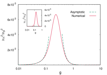
Figure 1: The solid line represents numerically evaluated ratio between $|c_{7}|^{2}$ and $|c_{3}|^{2}$. The dashed line represents the same ratio using their respective asymptotic expressions. Both for the large $g$ and small $g$, compared to $g_{0}$, the asymptotes closely follow the numerical results.

IV.5.2 Coefficient $c_{k}$ and energy gap $\Delta E_{k}$

In the Fock quantization the non-vanishing coefficient $c_{1}$ can be expressed using dimensionless parameter $g$ as $|c_{k}|^{2}\equiv|c_{1}|^{2}=\frac{1}{2}(l_{\star}/g)$. For the ease of comparison, we refer the coefficient $c_{3}$ as $c_{k}$ and the corresponding energy gap $\Delta E_{3}$ as $\Delta E_{k}$ also for polymer quantization. In the FIG.2, we have plotted the values $|c_{k}|^{2}$ as a function of the parameter $g$ using asymptotic expressions and numerically evaluated values.

In Fock quantization, the energy gap $\Delta E_{k}\equiv\Delta E_{3}=|\mathrm{k}|$ hence the ratio $\Delta E_{k}/|\mathrm{k}|$ is unity for all values of $g$. However, in polymer quantization, that ratio $\Delta E_{k}/|\mathrm{k}|$ deeps below unity and has a minima at around $g\approx 0.26$. In the region where $g\gg g_{0}$, this ratio differs drastically (22) from the result of Fock quantization. We have plotted the behaviour of the energy gap $\Delta E_{k}$ as a function of $g$ in FIG.2.

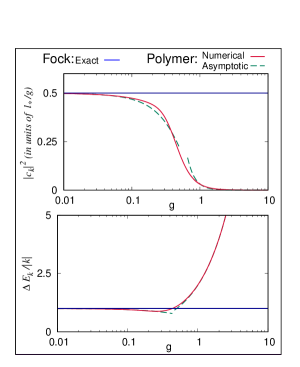
Figure 2: In Fock quantization, $|c_{k}|^{2}=\frac{1}{2}(l_{\star}/g)$ and it is represented as the solid blue line. The solid red line represents the numerical results and the dashed line represents the asymptotic expressions for $|c_{k}|^{2}$ in polymer quantization. In Fock quantization, $\Delta E_{3}/|\mathrm{k}|=1$, which is represented by the straight solid line. The curved solid line represents the numerical results and the dashed line represents asymptotic expressions for polymer quantization. For both small and large values of $g$, compared to $g_{0}$, the asymptotic expressions closely follow the numerical results.

IV.5.3 Wightman function

In order to perform the numerical evaluation, we scale the Wightman function as follows

$$G(\Delta t,\Delta\mathbf{x})=\frac{1}{4\pi^{2}l_{\star}^{2}}~{}\tilde{G}~{},$$ (58)

where $\tilde{G}$ is dimensionless. Using the equations (15) and (16), the regulated expression of the scaled and dimensionless Wightman function can be expressed as

$$\tilde{G}^{\epsilon}=\int_{g_{min}}^{g_{max}}dg~{}\tilde{h}(g,|\Delta\mathbf{x}|)~{}e^{-iu(g)-\epsilon g}.$$ (59)

where $g_{min}$ and $g_{max}$ are approximate limits of integration which are used in numerical evaluation to represent $0$ and $\infty$ respectively. The function $u(g)$ can be expressed in terms of the dimensionless quantities as

$$u(g)=g~{}\left(\frac{\Delta E_{k}}{|\mathrm{k}|}\right)~{}\left(\frac{\Delta t}{l_{\star}}\right)~{}.$$ (60)

Similarly, the function $\tilde{h}$ can be expressed in terms of dimensionless quantities as follows

$$\tilde{h}(g,|\Delta\mathbf{x}|)=2~{}\left(\frac{|c_{k}|^{2}g}{l_{\star}}\right)~{}\left(\frac{l_{\star}}{|\Delta\mathbf{x}|}\right)~{}\sin\left(g\frac{|\Delta\mathbf{x}|}{l_{\star}}\right)~{}.$$ (61)

It may be noted that we have explicitly expressed spacetime intervals $\Delta\mathbf{x}$ and $\Delta t$ in the units of $l_{\star}$.

From FIG.3, we may see that numerically evaluated Wightman function in polymer quantization, differs significantly from Fock quantization in short-distance. However, for the large distance they closely follow each other. Furthermore, in the limit $\Delta x^{2}\to 0$, numerically evaluated bounded value matches the asymptotic value $\tilde{G}_{0}\approx 0.24$.

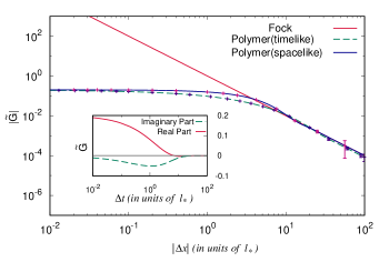
Figure 3: The Wightman function is scaled by a factor $1/4\pi^{2}l_{\star}^{2}$ and the solid red line represents the same in Fock quantization. The dashed green line represents absolute value of the scaled polymer Wightman function for timelike intervals and the solid blue line represents the same for spacelike intervals. For both timelike and spacelike intervals, the polymer Wightman function approaches the same value in the short distance. In large distance, Wightman function in polymer quantization mostly follows the result of the Fock quantization but in the short distance it differs significantly. The numerical error bars are amplified by a factor $10^{3}$ to make them legible in the figure. In the inset the solid red line represents the real part of the polymer Wightman function whereas the green dashed line represents the imaginary part.

IV.5.4 Numerical errors and the domain

The integrand in equation (59) involves exponential function. Therefore, by considering the limitation of double-precision floating-point numbers, here we have used $g_{min}=10^{-3}$ , $g_{max}=10^{3}$ for numerical evaluation of the Wightman function. To ensure the convergence of the integration (59) within the desired precision, we choose an appropriate value of the regulator $\epsilon$ which depends on $g_{max}$ as well as on the chosen intervals. In particular, for a given set of spatial interval $\Delta\mathbf{x}$ and temporal interval $\Delta t$, the regulator should be chosen such that $(u(g)/g\pm|\Delta\mathbf{x}|/l_{\star})>\epsilon$ and $(\epsilon~{}g_{max})>1$.

The numerical errors in computing Wightman function stems from the finite size of the divisions that we consider for integrating using trapezoidal rule. Therefore, we can estimate this numerical errors by computing the same integral using two different division sizes and then considering their differences as follows

$$\delta G_{num}=|G|_{\Delta g_{1}}-|G|_{\Delta g_{2}}~{}.$$ (62)

Here we have considered $\Delta g_{1}=2\times 10^{-4}$ and $\Delta g_{2}=1\times 10^{-4}$. It can be seen from FIG. 3 that the numerical errors are much smaller than the evaluated values of the Wightman function for both the cases.

V Discussions

In summary, we have studied the properties of the Wightman function i.e. vacuum two-point function, corresponding to a massless free scalar field in polymer quantization. In Fock quantization, the corresponding Wightman function is inversely proportional to the invariant distance squared between the corresponding spacetime points. Therefore, the Wightman function diverges when these two points are taken to be infinitesimally close to each other. We have shown here that in contrast to the Fock quantization, Wightman function is bounded from above in polymer quantization. We have established this bounded nature of the Wightman function by asymptotic but analytic computation as well as using numerical methods. The bounded value of the polymer Wightman function is controlled by the polymer length scale $l_{\star}$ which is analogous to the Planck length.

We have argued that the Wightman function i.e. vacuum two-point function, can be used as a probe to measure the effective spacetime distance between these two points, as experienced by the scalar field. In the case of polymer quantization, the bounded Wightman function leads to the notion of zero-point length of spacetime. Such notion of the zero-point length has long been anticipated to arise from the possible quantum gravity effects quite generically Padmanabhan (1997); Smailagic et al. (2003) as well as in specific approaches to quantum gravity such as in string theory Amati et al. (1989); Gross and Mende (1988); YONEYA (1989), non-commutative geometry Girelli et al. (2005); Douglas and Nekrasov (2001). However, in this article we have used polymer quantization only for matter field and the geometry has been treated classically. In this sense, the polymer quantization of matter field itself seems to capture certain aspects of quantum gravity effects. In other words, the property of the Wightman function in polymer quantization seems to imply an emergence of an effective discreteness in the spacetime.

We now discuss few implications of this bounded nature of the Wightman function. In the study of Unruh effect, the properties of the Wightman function plays an important role. In particular, the non-transient term of the instantaneous transition rate of the Unruh-DeWitt detector contains a residue evaluated at the pole of the Wightman function. In contrast to the Fock quantization, there is no pole in polymer Wightman function as shown here. Therefore, the non-transient term in the response function of the Unruh-Dewitt detector would disappear in polymer quantization Hossain and Sardar (2016b). Nevertheless, there are some alternative views on the response of the Unruh-DeWitt detectors Kajuri (2016); Husain and Louko (2016). The properties of the Wightman function as shown here also support the results of Hossain and Sardar (2015) where the violation of Kubo-Martin-Schwinger condition is shown and criticism raised in Rovelli (2014) is addressed. The disappearance of the Unruh effect has also been seen using the method of Bogoliubov transformation Hossain and Sardar (2016a). The bounded nature of the Wightman function also serves as an example where some aspects of the anticipation regarding quantum gravity to serve as a natural regulator Garay (1995); Hossenfelder (2013, 2006, 2004); Thiemann (1998); Kothawala (2013), are realized.

We may also like to point out that the bounded nature of the Wightman function as shown here, is analogous to the behaviour of the effective Hubble parameter and the spectrum of inverse scale factor operator in loop quantum cosmology (LQC) Ashtekar et al. (2006a, b); Bojowald (2001a, b). These results are also associated with some inverse powers of the distance scale, similar to the properties of the two-point function. In LQC, this crucial behaviour plays a key role in resolution of Big Bang singularity. However unlike in LQC, here we have applied polymer quantization only for scalar matter field rather than for the geometry.