On the Laplacian spectra of some double join operations of graphs

Abstract

Many variants of join operations of graphs have been introduced and their spectral properties have been studied extensively by many researchers. This paper mainly focuses on the Laplacian spectra of some double join operations of graphs. We first introduce the conception of double join matrix and provide a complete information about its eigenvalues and the corresponding eigenvectors. Further, we define four variants of double join operations based on subdivision graph, $Q$-graph, $R$-graph and total graph. Applying the result obtained for the double join matrix, we give an explicit complete characterization of the Laplacian eigenvalues and the corresponding eigenvectors of four variants in terms of the Laplacian eigenvalues and the eigenvectors of the factor graphs. These results generalize some well-known results about some join operations of graphs.

AMS classification: 05C50 05C90 15A18

Key words: Double join matrix; Laplacian matrix; Laplacian spectrum; Laplacian eigenvector; Join operations

1. Introduction

Throughout this paper, all graphs considered are finite simple graphs. Let $G=(V,E)$ be a graph with vertex set $V=\{v_{1},v_{2},\ldots,v_{n}\}$ and edge set $E(G)$. The adjacency matrix $A(G)=(a_{ij})$ of $G$ is an $n\times n$ matrix where $a_{ij}=1$ whenever $v_{i}$ and $v_{j}$ are adjacent in $G$ and $a_{ij}=0$ otherwise. The degree of $v_{i}$ in $G$ is denoted by $d_{i}=d_{G}(v_{i})$. Let $D(G)$ be the degree diagonal matrix of $G$ with diagonal entries $d_{1},d_{2},\ldots,d_{n}$. The Laplacian matrix $L(G)$ of $G$ is defined as $D(G)-A(G)$. The signless Laplacian matrix of $G$ is defined as $|L|(G)=D(G)+A(G)$. For an $n\times n$ matrix $M$ associated to $G$, the set of all the eigenvalues of $M$ is called the spectrum of matrix $M$ or graph $G$. In particular, if $M$ is the adjacency matrix $A(G)$ of $G$, then the adjacency spectrum of $G$ is denoted by $\sigma(A(G))=(\nu_{1}(G),\nu_{2}(G),\ldots,\nu_{n}(G)),$ where $\nu_{1}(G)\leq\nu_{2}(G)\leq\cdots\leq\nu_{n}(G)$ are the eigenvalues of $A(G)$. If $M$ is the Laplacian matrix $L(G)$ of $G$, then the Laplacian spectrum of $G$ is denoted by $\sigma(L(G))=(\lambda_{1}(G),\lambda_{2}(G),\ldots,\lambda_{n}(G)),$ where $\lambda_{1}(G)\leq\lambda_{2}(G)\leq\cdots\leq\lambda_{n}(G)$ are the eigenvalues of $L(G)$. If $M$ is the signless Laplacian matrix $|L|(G)$ of $G$, then the signless Laplacian spectrum of $G$ is denoted by $\sigma(|L|(G))=(q_{1}(G),q_{2}(G),\ldots,q_{n}(G)),$ where $q_{1}(G)\leq q_{2}(G)\leq\cdots\leq q_{n}(G)$ are the eigenvalues of $|L|(G)$. For more review about the adjacency spectrum, Laplacian spectrum and signless Laplacian spectrum of $G$, readers may refer to [5, 7, 9, 10, 11, 13, 18] and the references therein.

Determining the spectra of many graph operations is a basic and very meaningful work in spectral graph theory. Up till now, many graph operations such as Cartesian product, Kronecker product, graph with $k$ (edge)-pockets, corona, edge corona, some variants of (edge)corona, join, some variants of join have been introduced and the adjacency spectra (Laplacian spectra, signless Laplacian spectra as well) of these graph operations have also been determined in terms of the corresponding spectra of the factor graphs in [1, 2, 3, 4, 6, 8, 12, 14, 15, 16, 20, 21]. Moreover, it is known that the corresponding spectra of these graph operations can be used to construct infinitely many pairs of cospectral graphs[1, 3, 4, 8, 11, 16, 20], infinitely families of integral graphs[2, 15] and to investigate many other properties of graphs, such as the Kirchhoff index[16, 17, 21], the number of spanning trees[4, 14, 16] and so on. This paper focuses on the Laplacian spectra of four new variants of double join operations based on subdivision graph, $Q$-graph, $R$-graph and total graph. The following definitions come from [9], which will be required to define our new operations.

Let $G$ be a connected graph with $n$ vertices and $m$ edges. The subdivision graph $S(G)$ is the graph obtained by inserting a new vertex into every edge of $G$. The $Q$-graph $Q(G)$ is the graph obtained by inserting a new vertex into every edge of $G$ and by adding edges between those inserted vertex which lie on adjacent edges of $G$. The $R$-graph $R(G)$ is the graph by adding a new vertex corresponding to each edge of $G$ and by adding edges between each added vertex and the corresponding edge’s endpoints. The total graph $T(G)$ is the graph whose vertex set is the union of vertex set and edge set of $G$, and two vertex of $T(G)$ is adjacent whenever two corresponding elements are incident or adjacent; see Figure 1 for example.

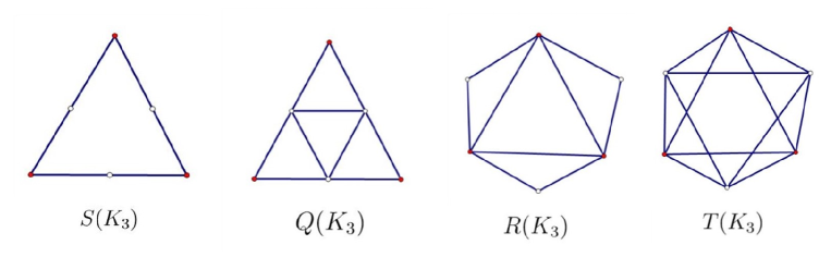
Figure 1: $S(K_{3})$, $Q(K_{3})$, $R(K_{3})$ and $T(K_{3})$ for the complete graph $K_{3}$. (Here new added vertices are white, the old vertices are black.)

Definition 1.

Let $G$ be a connected graph with $n$ vertices and $m$ edges. Also let $G_{1}$ and $G_{2}$ be two graphs with $n_{1}$ and $n_{2}$ vertices, respectively. The subdivision double join $G^{S}\vee{(G^{\bullet}_{1},G^{\circ}_{2})}$ of $G$ , $G_{1}$ and $G_{2}$ is the graph obtained from $S(G)$, $G_{1}$ and $G_{2}$ by joining every vertex of $G$ to every vertex of $G_{1}$ and every vertex of $I(G)$ to every vertex of $G_{2}$, where $I(G)$ denotes the vertex set of the added new vertices in $S(G)$. Replaced $S(G)$ by $Q(G)$ ($R(G),T(G)$) in this definition, the resulting graph is referred to as $Q$-graph($R$-graph, total, respectively) double join of these graphs. Similarly, we denote them by $G^{Q}\vee{(G^{\bullet}_{1},G^{\circ}_{2})}$, $G^{R}\vee{(G^{\bullet}_{1},G^{\circ}_{2})}$ and $G^{T}\vee{(G^{\bullet}_{1},G^{\circ}_{2})}$, respectively.

Example 2.

Let $G$, $G_{1}$ and $G_{2}$ be the complete graph $K_{3}$, the paths $P_{2}$ and $P_{3}$, respectively. Figure 2 displays four graphs $K_{3}^{S}\vee{(P_{2}^{\bullet},P_{3}^{\circ})}$, $K_{3}^{Q}\vee{(P_{2}^{\bullet},P_{3}^{\circ})}$, $K_{3}^{R}\vee{(P_{2}^{\bullet},P_{3}^{\circ})}$ and $K_{3}^{T}\vee{(P_{2}^{\bullet},P_{3}^{\circ})}$ below.

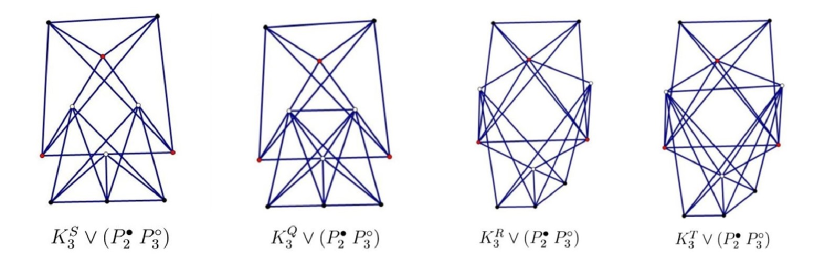
Figure 2: Illustration of $K_{3}^{S}\vee{(P_{2}^{\bullet},P_{3}^{\circ})}$, $K_{3}^{Q}\vee{(P_{2}^{\bullet},P_{3}^{\circ})}$, $K_{3}^{R}\vee{(P_{2}^{\bullet},P_{3}^{\circ})}$ and $K_{3}^{T}\vee{(P_{2}^{\bullet},P_{3}^{\circ})}$ in Example 2.

Recently, many variants of join operations of graphs have been introduced and their spectral properties have been studied by many researchers. Cardoso et al.[6] characterized adjacency and Laplacian spectra of the $H$-join operation of graphs. Estrada and Benzi[12] discussed the clustering, assortativity and spectral properties of core-satellite graphs. Remark that the core-satellite graph named in [12] is a special join of some complete graphs. In [15], the adjacency spectra of the subdivision vertex(edge) joins of graphs were computed in terms of the corresponding spectra of two regular graphs. The author also constructed infinite family of new integral graphs. Liu and Zhang[16] determined the spectra, (signless) Laplacian spectra of the subdivision vertex(edge) joins for a regular graph $G_{1}$ and arbitrary graph $G_{2}$. As applications, they constructed infinitely many pairs of cospectral graphs and obtained the number of spanning trees and the Kirchhoff index of the subdivision vertex(edge) joins. Remark that they determined these spectra with the help of the coronal technique. But this technique cannot describe completely the eigenvectors corresponding to all the eigenvalues.

Motivated by these researches, we discuss the Laplacian spectra of four new variants of double join operations based on subdivision graph, $Q$-graph, $R$-graph and total graph namely, $G^{S}\vee{(G^{\bullet}_{1},G^{\circ}_{2})}$, $G^{Q}\vee{(G^{\bullet}_{1},G^{\circ}_{2})}$, $G^{R}\vee{(G^{\bullet}_{1},G^{\circ}_{2})}$ and $G^{T}\vee{(G^{\bullet}_{1},G^{\circ}_{2})}$. The rest of this paper is organized as follows. In Section 2, we shall introduce the conception of double join matrix and provide a complete information about its eigenvalues and the corresponding eigenvectors. In Section 3, applying the result obtained for the double join matrix, we give an explicit complete characterization of the Laplacian spectra of the four variants $G^{S}\vee{(G^{\bullet}_{1},G^{\circ}_{2})}$, $G^{Q}\vee{(G^{\bullet}_{1},G^{\circ}_{2})}$, $G^{R}\vee{(G^{\bullet}_{1},G^{\circ}_{2})}$ and $G^{T}\vee{(G^{\bullet}_{1},G^{\circ}_{2})}$ in terms of the Laplacian spectra of the factor graphs. These results not only generalize some well-known results, but also describe completely the eigenvectors corresponding to all the Laplacian eigenvalues of these graphs. In Section 4, we summarize our work and give some further remarks.

2. Spectra of double join matrices

Suppose that $A$, $C$, $D$, $E$ are real matrices of order $p$, $q$, $r$, $s$, respectively and $B$ is a $p\times q$ matrix with $p<q$. Consider the following block matrix:

$$\mathscr{D}_{j}=\begin{pmatrix}A&B&cJ_{p\times r}&\textbf{0}_{p\times s}\\ B^{T}&C&\textbf{0}_{q\times r}&cJ_{q\times s}\\ cJ_{r\times p}&\textbf{0}_{r\times q}&D&\textbf{0}_{r\times s}\\ \textbf{0}_{s\times p}&cJ_{s\times q}&\textbf{0}_{s\times r}&E\\ \end{pmatrix},$$

where $J_{p\times r}$ denotes the $p\times r$ matrix with every entry is equal to 1 and $c=\pm 1$. Obviously, $\mathscr{D}_{j}$ is a matrix of order $p+q+r+s$. Throughout $\textbf{1}_{n}$ denotes the column vector of order $n$ with every entry 1. We call $\mathscr{D}_{j}$ the double join matrix if $\mathscr{D}_{j}$ satisfies the following four conditions:

1. If $\textbf{X}_{i}$ and $\textbf{Y}_{i}$ are the singular vector pairs of $B$ corresponding to the singular values $b_{i}$ for $i=1,2,...,p$, then $\textbf{X}_{i}$ and $\textbf{Y}_{i}$ are the orthogonal unit eigenvectors of $A$ and $C$. Equivalently, $B\textbf{Y}_{i}=b_{i}\textbf{X}_{i}$ and $B^{T}\textbf{X}_{i}=b_{i}\textbf{Y}_{i}$ for $i=1,2,...,p$ imply $A\textbf{X}_{i}=a_{i}\textbf{X}_{i}$, $C\textbf{Y}_{i}=c_{i}\textbf{Y}_{i}$ where $a_{i}$ and $c_{i}$ are eigenvalues of matrices $A$ and $C$, respectively.

2. Assume that $\textbf{X}_{1}=\frac{1}{\sqrt{p}}\textbf{1}_{p}$ and $\textbf{Y}_{1}=\frac{1}{\sqrt{q}}\textbf{1}_{q}$ are the unit eigenvectors of $A$ and $C$ corresponding to the eigenvalues $a_{1}$ and $c_{1}$, respectively.

3. If $B\textbf{Y}_{j}=\textbf{0}_{p}$ for $j=p+1,p+2,...,q$, then $\textbf{Y}_{j}$ are the orthogonal eigenvectors of $C$, that is, $C\textbf{Y}_{j}=c_{j}\textbf{Y}_{j}$ for $j=p+1,p+2,...,q$, where $c_{j}$ are eigenvalues of $C$.

4. Also assume that $\textbf{Z}_{1}=\frac{1}{\sqrt{r}}\textbf{1}_{r}$ and $\textbf{W}_{1}=\frac{1}{\sqrt{s}}\textbf{1}_{s}$ are the unit eigenvectors of $D$ and $E$ corresponding to the eigenvalues $d_{1}$ and $e_{1}$, respectively.

Next, we shall give a full description of all the eigenvalues and the corresponding eigenvectors for the double join matrix $\mathscr{D}_{j}$.

Theorem 3.

The spectrum of the double join matrix $\mathscr{D}_{j}$ consists of:

• The eigenvalues $\lambda=d_{i}$ for $i=2,3,...,r$;

• The eigenvalues $\lambda=e_{i}$ for $i=2,3,...,s$;

• The eigenvalues $\lambda_{\pm}=\frac{a_{i}+c_{i}\pm\sqrt{(a_{i}-c_{i})^{2}+4b_{i}^{2}}}{2}$ for $i=2,3,...,p$;

• The eigenvalues $\lambda=c_{j}$ for $j=p+1,p+2,...,q$;

• The remaining four eigenvalues are given by the roots of the following equation:
  $\lambda^{4}-(e_{1}+c_{1}+a_{1}+d_{1})\lambda^{3}+(e_{1}c_{1}-qs+(a_{1}+d_{1})(e_{1}+c_{1})+a_{1}d_{1}-pr-b^{2}_{1})\lambda^{2}+((d_{1}+e_{1})b^{2}_{1}-(a_{1}+d_{1})(e_{1}c_{1}-qs)-(a_{1}d_{1}-pr)(e_{1}+c_{1}))\lambda+(a_{1}d_{1}-pr)(e_{1}c_{1}-qs)-d_{1}e_{1}b^{2}_{1}=0.$

Proof.

Suppose that $\textbf{Z}_{1},\textbf{Z}_{2},\ldots,\textbf{Z}_{r}$ are the orthogonal eigenvectors of $D$ corresponding to the eigenvalues $d_{1},d_{2},...,d_{r}$, respectively. Firstly, consider the vectors

$$\;\;\;\;\;\;\;\;\;\;\;\;\;\;\;\;\;\;\;\;\;\;\;\;\;\;\;\;\;\;\;\;\;\textbf{x}=\begin{pmatrix}\textbf{0}_{p}\\ \textbf{0}_{q}\\ \textbf{Z}_{i}\\ \textbf{0}_{s}\\ \end{pmatrix},\;\;\;\text{for}~{}i=2,3,...,r.$$ (1)

Notice that $J_{p\times r}\textbf{Z}_{i}=\textbf{0}_{p}$ as $\textbf{Z}_{i}\bot\textbf{1}_{r}$. Then the equation $\mathscr{D}_{j}\textbf{x}=\lambda\textbf{x}$ becomes

$$\mathscr{D}_{j}\textbf{x}=\begin{bmatrix}\textbf{0}_{p}\\ \textbf{0}_{q}\\ d_{i}\textbf{Z}_{i}\\ \textbf{0}_{s}\\ \end{bmatrix}=\begin{bmatrix}\textbf{0}_{p}\\ \textbf{0}_{q}\\ \lambda\textbf{Z}_{i}\\ \textbf{0}_{s}\\ \end{bmatrix}.$$

So, $\lambda=d_{i}$ are the eigenvalues of double join matrix $\mathscr{D}_{j}$ for $i=2,3...,r$.

Now suppose that $\textbf{W}_{1},\textbf{W}_{2},\ldots,\textbf{W}_{s}$ are the orthogonal eigenvectors of $E$ corresponding to the eigenvalues $e_{1},e_{2},...,e_{s}$, respectively. Next, consider the vectors

$$\;\;\;\;\;\;\;\;\;\;\;\;\;\;\;\;\;\;\;\;\;\;\;\;\;\;\;\;\;\;\;\;\;\textbf{x}=\begin{pmatrix}\textbf{0}_{p}\\ \textbf{0}_{q}\\ \textbf{0}_{r}\\ \textbf{W}_{i}\\ \end{pmatrix},\;\;\;\text{for}~{}i=2,3,...,s.$$ (2)

Then we plug (2) into the equation $\mathscr{D}_{j}\textbf{x}=\lambda\textbf{x}$. Notice that $J_{q\times s}\textbf{W}_{i}=\textbf{0}_{q}$ as $\textbf{W}_{i}\bot\textbf{1}_{s}$. Thus one gets

$$\mathscr{D}_{j}\textbf{x}=\begin{bmatrix}\textbf{0}_{p}\\ \textbf{0}_{q}\\ \textbf{0}_{r}\\ e_{i}\textbf{W}_{i}\\ \end{bmatrix}=\begin{bmatrix}\textbf{0}_{p}\\ \textbf{0}_{q}\\ \textbf{0}_{r}\\ \lambda\textbf{W}_{i}\\ \end{bmatrix}.$$

So, $\lambda=e_{i}$ ($i=2,3,...,s$) are also eigenvalues of double join matrix $\mathscr{D}_{j}$.

Now consider the following vectors

$$\;\;\;\;\;\;\;\;\;\;\;\;\;\;\;\;\;\;\;\;\;\;\;\;\;\;\;\;\;\;\;\;\;\textbf{x}=\begin{pmatrix}k_{1}\textbf{X}_{i}\\ \textbf{Y}_{i}\\ \textbf{0}_{r}\\ \textbf{0}_{s}\\ \end{pmatrix},\;\;\;\text{for}~{}i=2,3,...,p,$$ (3)

where $k_{1}$ is an unknown constant to be determined. Notice that $J_{r\times p}\textbf{X}_{i}=\textbf{0}_{r}$ and $J_{s\times q}\textbf{Y}_{i}=\textbf{0}_{s}$ as $\textbf{X}_{i}\bot\textbf{1}_{p}$ and $\textbf{Y}_{i}\bot\textbf{1}_{q}$. Again, plugging (3) into the equation $\mathscr{D}_{j}\textbf{x}=\lambda\textbf{x}$, we obtain

$$\mathscr{D}_{j}\textbf{x}=\begin{bmatrix}k_{1}a_{i}\textbf{X}_{i}+b_{i}\textbf{X}_{i}\\ k_{1}b_{i}\textbf{Y}_{i}+c_{i}\textbf{Y}_{i}\\ \textbf{0}_{r}\\ \textbf{0}_{s}\\ \end{bmatrix}=\lambda\begin{bmatrix}k_{1}\textbf{X}_{i}\\ \textbf{Y}_{i}\\ \textbf{0}_{r}\\ \textbf{0}_{s}\\ \end{bmatrix},$$

which reduces to the following conditions

$$k_{1}a_{i}+b_{i}=\lambda k_{1},\;\;\;k_{1}b_{i}+c_{i}=\lambda.$$

Eliminating $k_{1}$ from above conditions, one obtains

$$\;\;\;\;\;\;\;\;\;\;\;\;\;\;\;\;\;\;\;\;\;\;\;\;\;\;\;\;\;\;\lambda^{2}-(a_{i}+c_{i})\lambda+a_{i}c_{i}-b_{i}^{2}=0.$$ (4)

The roots of the equation (4) are $\lambda_{\pm}=\frac{(a_{i}+c_{i})\pm\sqrt[2]{(a_{i}-c_{i})^{2}+4b_{i}^{2}}}{2}$, which implies that the third part of theorem follows.

Below, we consider the vectors

$$\;\;\;\;\;\;\;\;\;\;\;\;\;\;\;\;\;\;\;\;\;\;\;\;\;\;\;\;\;\;\;\;\;\textbf{x}=\begin{pmatrix}\textbf{0}_{p}\\ \textbf{Y}_{j}\\ \textbf{0}_{r}\\ \textbf{0}_{s}\\ \end{pmatrix},\;\;\;\text{for}~{}j=p+1,p+2,...,q.$$ (5)

Observe that $B\textbf{Y}_{j}=\textbf{0}_{p}$ and $J_{s\times q}\textbf{Y}_{j}=\textbf{0}_{s}$ for $j=p+1,p+2,...,q$. Then the equation $\mathscr{D}_{j}\textbf{x}=\lambda\textbf{x}$ becomes

$$\mathscr{D}_{j}\textbf{x}=\begin{bmatrix}\textbf{0}_{p}\\ c_{j}\textbf{Y}_{j}\\ \textbf{0}_{r}\\ \textbf{0}_{s}\\ \end{bmatrix}=\lambda\begin{bmatrix}\textbf{0}_{p}\\ \textbf{Y}_{j}\\ \textbf{0}_{r}\\ \textbf{0}_{s}\\ \end{bmatrix}.$$

Hence, $\lambda=c_{j}$ ($j=p+1,p+2,...,q$) are eigenvalues of $\mathscr{D}_{j}$. So far we have determined $p+q+r+s-4$ eigenvalues of $\mathscr{D}_{j}$.

To determine the four remaining eigenvalues and the corresponding eigenvectors, let

$$\;\;\;\;\;\;\;\;\;\;\;\;\;\;\;\;\;\;\;\;\;\;\;\;\;\;\;\;\;\;\;\;\;\;\;\;\;\;\;\;\;\;\;\textbf{x}=\begin{pmatrix}k_{1}\textbf{1}_{p}\\ k_{2}\textbf{1}_{q}\\ k_{3}\textbf{1}_{r}\\ \textbf{1}_{s}\\ \end{pmatrix},$$ (6)

where $k_{1},k_{2},k_{3}$ are three unknown constants to be determined. Note that $B\textbf{1}_{q}=\sqrt{q}B\frac{\textbf{1}_{q}}{\sqrt{q}}=b_{1}\sqrt{\frac{q}{p}}\textbf{1}_{p}$ and $B^{T}\textbf{1}_{p}=b_{1}\sqrt{\frac{p}{q}}\textbf{1}_{q}$. Plugging (6) into the equation $\mathscr{D}_{j}\textbf{x}=\lambda\textbf{x}$, we get following conditions.

$$\begin{cases}k_{1}a_{1}+k_{2}b_{1}\sqrt{\frac{q}{p}}+ck_{3}r=\lambda k_{1},\\ k_{1}\sqrt{\frac{p}{q}}b_{1}+k_{2}c_{1}+cs=\lambda k_{2},\\ ck_{1}p+k_{3}d_{1}=\lambda k_{3},\\ ck_{2}q+e_{1}=\lambda.\\ \end{cases}$$

Eliminating $k_{1},k_{2}$ and $k_{3}$ from above conditions, one obtains

$$(\lambda-a_{1}-\frac{c^{2}pr}{\lambda-d_{1}})(\lambda-c_{1}-\frac{c^{2}qs}{\lambda-e_{1}})=b_{1}^{2}.$$

Note $c^{2}=1$. We may reduce this equation to

$\lambda^{4}-(e_{1}+c_{1}+a_{1}+d_{1})\lambda^{3}+(e_{1}c_{1}-qs+(a_{1}+d_{1})(e_{1}+c_{1})+a_{1}d_{1}-pr-b^{2}_{1})\lambda^{2}+((d_{1}+e_{1})b^{2}_{1}-(a_{1}+d_{1})(e_{1}c_{1}-qs)-(a_{1}d_{1}-pr)(e_{1}+c_{1}))\lambda+(a_{1}d_{1}-pr)(e_{1}c_{1}-qs)-d_{1}e_{1}b^{2}_{1}=0.$

The proof of this theorem is completed. ∎

3. Laplacian spectra of double join operations of graphs

In this section, applying the result obtained in Theorem 3, we shall give an explicit complete characterization of the Laplacian spectra of four variants of the double join operations $G^{S}\vee{(G^{\bullet}_{1},G^{\circ}_{2})}$, $G^{Q}\vee{(G^{\bullet}_{1},G^{\circ}_{2})}$, $G^{R}\vee{(G^{\bullet}_{1},G^{\circ}_{2})}$ and $G^{T}\vee{(G^{\bullet}_{1},G^{\circ}_{2})}$ in terms of the Laplacian spectra of the factor graphs.

We first focus on determining the Laplacian spectra of the subdivision double join $G^{S}\vee{(G^{\bullet}_{1},G^{\circ}_{2})}$ for a regular graph $G$ and two arbitrary graphs $G_{1}$, $G_{2}$.

Theorem 4.

Let $G$ be a $k$-regular graph with $n$ vertices and $m$ edges. Also let $G_{1}$ and $G_{2}$ be two arbitrary graph with $n_{1}$ and $n_{2}$ vertices, respectively. Then the Laplacian spectrum of $G^{S}\vee{(G^{\bullet}_{1},G^{\circ}_{2})}$ consists of:

1. $\lambda_{i}(G_{1})+n$, for $i=2,3,...,n_{1}$;

2. $\lambda_{i}(G_{2})+m$, for $i=2,3,...,n_{2}$;

3. $\frac{(n_{1}+k+n_{2}+2)\pm\sqrt{(n_{1}+k-n_{2}-2)^{2}+4(2k-\lambda_{i}(G))}}{2}$ , for $i=2,3,...,n$;

4. $n_{2}+2$, repeated $m-n$ times;

5. all the roots of the following equation
   $\lambda(\lambda^{3}-(m+n+n_{1}+k+n_{2}+2)\lambda^{2}+(2m+(n_{1}+k+n)(m+n_{2}+2)+nk-2k)\lambda+2(n+m)k-2(n_{1}+k+n)m-nk(m+n_{2}+2))=0$.

Proof.

With a suitable labeling of the vertices of $G^{S}\vee{(G^{\bullet}_{1},G^{\circ}_{2})}$, we can write the Laplacian matrix of $G^{S}\vee{(G^{\bullet}_{1},G^{\circ}_{2})}$ as

$$L(G^{S}\vee{(G^{\bullet}_{1},G^{\circ}_{2})})=\begin{pmatrix}(n_{1}+k)I_{n}&-M&-J_{n\times n_{1}}&\textbf{0}_{n\times n_{2}}\\ -M^{T}&(n_{2}+2)I_{m}&\textbf{0}_{m\times n_{1}}&-J_{m\times n_{2}}\\ -J_{n_{1}\times n}&\textbf{0}_{n_{1}\times m}&L(G_{1})+nI_{n_{1}}&\textbf{0}_{n_{1}\times n_{2}}\\ \textbf{0}_{n_{1}\times n}&-J_{n_{2}\times m}&\textbf{0}_{n_{2}\times n_{1}}&L(G_{2})+mI_{n_{2}}\\ \end{pmatrix},$$

where $M$ denotes vertex-edge incidence matrix of $G$ and $I_{n}$ the identity matrix of order $n$. By comparing the Laplacian matrix $L(G^{S}\vee{(G^{\bullet}_{1},G^{\circ}_{2})})$ with the double join matrix $\mathscr{D}_{j}$, we take $p=n$, $q=m$, $r=n_{1}$, $s=n_{2}$, $c=-1$ and $A=(n_{1}+k)I_{n}$, $B=-M$, $C=(n_{2}+2)I_{m}$, $D=L(G_{1})+nI_{n_{1}}$, $E=L(G_{2})+mI_{n_{2}}$ in Theorem 3. Since $MM^{T}=\left|L\right|\left(G\right)=kI_{n}+A(G)=2kI_{n}-L(G)$, $L(G_{1})\textbf{1}_{n_{1}}=0\textbf{1}_{n_{1}}$ and $L(G_{2})\textbf{1}_{n_{2}}=0\textbf{1}_{n_{2}}$. Then we have

• $a_{i}=n_{1}+k$ for $i=1,2,...,n$,   $a_{1}=n_{1}+k$;

• $b_{i}^{2}=2k-\lambda_{i}(G)$ for $i=1,2,...,n$,   $b_{1}^{2}=2k$;

• $c_{i}=n_{2}+2$ for $i=1,2,...,m$;

• $d_{i}=\lambda_{i}(G_{1})+n$ for $i=1,2,...,n_{1}$,   $d_{1}=n$;

• $e_{i}=\lambda_{i}(G_{2})+m$ for $i=1,2,...,n_{2}$,   $e_{1}=m$.

Now plugging these values into Theorem 3, we obtain the required result. ∎

Remark 5.

Remark that the subdivision double join $G^{S}\vee{(G^{\bullet}_{1},G^{\circ}_{2})}$ becomes the subdivision-vertex join defined in [15] whenever $G_{2}$ is a null graph. Similarly, the subdivision double join $G^{S}\vee{(G^{\bullet}_{1},G^{\circ}_{2})}$ becomes the subdivision-edge join defined in [15] whenever $G_{1}$ is a null graph. In [16], Liu and Zhang determined the Laplacian spectra of subdivision-vertex join and subdivision-edge join. Clearly, Theorem 4 generalizes the results of both Theorems 2.7 and 3.4 in [16].

Next, we give a complete description of the Laplacian spectra of the $Q$-graph double join $G^{Q}\vee{(G^{\bullet}_{1},G^{\circ}_{2})}$ for a regular graph $G$ and two arbitrary graphs $G_{1}$, $G_{2}$.

Theorem 6.

Let $G$ be a $k$-regular graph with $n$ vertices and $m$ edges. Also let $G_{1}$ and $G_{2}$ be two arbitrary graph with $n_{1}$ and $n_{2}$ vertices, respectively. Then the Laplacian spectrum of $G^{Q}\vee{(G^{\bullet}_{1},G^{\circ}_{2})}$ consists of:

1. $\lambda_{i}(G_{1})+n$, for $i=2,3,...,n_{1}$;

2. $\lambda_{i}(G_{2})+m$, for $i=2,3,...,n_{2}$;

3. $\frac{(n_{1}+k+n_{2}+2+\lambda_{i}(G))\pm\sqrt{(n_{1}+k-n_{2}-2-\lambda_{i}(G))^{2}+4(2k-\lambda_{i}(G))}}{2}$ , for $i=2,3,...,n$;

4. $n_{2}+2k+2$, repeated $m-n$ times;

5. four roots of the equation
   $\lambda(\lambda^{3}-(m+n+n_{1}+k+n_{2}+2)\lambda^{2}+(2m+(n_{1}+k+n)(m+n_{2}+2)+nk-2k)\lambda+2(n+m)k-2(n_{1}+k+n)m-nk(m+n_{2}+2))=0.$

Proof.

With a proper labeling of vertices, the Laplacian matrix of $G^{Q}\vee{(G^{\bullet}_{1},G^{\circ}_{2})}$ can be written as

$$L(G^{Q}\vee{(G^{\bullet}_{1},G^{\circ}_{2})})=\begin{pmatrix}(n_{1}+k)I_{n}&-M&-J_{n\times n_{1}}&\textbf{0}_{n\times n_{2}}\\ -M^{T}&(n_{2}+2)I_{m}+L(l(G))&\textbf{0}_{m\times n_{1}}&-J_{m\times n_{2}}\\ -J_{n_{1}\times n}&\textbf{0}_{n_{1}\times m}&L(G_{1})+nI_{n_{1}}&\textbf{0}_{n_{1}\times n_{2}}\\ \textbf{0}_{n_{1}\times n}&-J_{n_{2}\times m}&\textbf{0}_{n_{2}\times n_{1}}&L(G_{2})+mI_{n_{2}}\\ \end{pmatrix},$$

where $l(G)$ denotes the line graph of $G$.

Now, comparing the Laplacian matrix $L(G^{Q}\vee{(G^{\bullet}_{1},G^{\circ}_{2})})$ with the double join matrix $\mathscr{D}_{j}$, we take $A=(n_{1}+k)I_{n}$, $B=-M$, $C=(n_{2}+2)I_{m}+L(l(G))$, $D=L(G_{1})+nI_{n_{1}}$, $E=L(G_{2})+mI_{n_{2}}$ in Theorem 3. Since $D(l(G))=2(k-1)I_{m}$, $A(l(G))=M^{T}M-2I_{m}$. Then $L(l(G))=2kI_{m}-M^{T}M$, which implies that $C=(n_{2}+2k+2)I_{m}-M^{T}M$. Note that $MM^{T}=2kI_{n}-L(G)$. Since $MM^{T}$ and $M^{T}M$ have same nonzero eigenvalues. Then the spectrum of $C$ consists of: $c_{i}=n_{2}+\lambda_{i}(G)+2$ for $i=1,2,...,n$ and $c_{j}=n_{2}+2k+2$ for $j=n+1,n+2,...,m$. Furthermore, it follows from Theorem 3.38 in [9] that $C\textbf{Y}_{j}=c_{j}\textbf{Y}_{j}$ satisfy $M\textbf{Y}_{j}=\textbf{0}_{n}$ for $j=n+1,n+2,...,m$. Therefore, one has

• $a_{i}=n_{1}+k$ for $i=1,2,...,n$,   $a_{1}=n_{1}+k$;

• $b_{i}^{2}=2k-\lambda_{i}(G)$ for $i=1,2,...,n$,   $b_{1}^{2}=2k$;

• $c_{i}=n_{2}+\lambda_{i}(G)+2$ for $i=1,2,...,n$,  $c_{j}=n_{2}+2k+2$ for $j=n+1,...,m$;

• $d_{i}=\lambda_{i}(G_{1})+n$ for $i=1,2,...,n_{1}$,   $d_{1}=n$;

• $e_{i}=\lambda_{i}(G_{2})+m$ for $i=1,2,...,n_{2}$,   $e_{1}=m$.

Now from Theorem 3, the required result follows. ∎

The following result describes the Laplacian spectra of the $R$-graph double join $G^{R}\vee{(G^{\bullet}_{1},G^{\circ}_{2})}$ for a regular graph $G$ and two arbitrary graphs $G_{1}$, $G_{2}$.

Theorem 7.

Let $G$ be a $k$-regular graph with $n$ vertices and $m$ edges. Let $G_{1}$ and $G_{2}$ be two arbitrary graph witn $n_{1}$ and $n_{2}$ vertices, respectively. Then the Laplacian spectrum of $G^{R}\vee{(G^{\bullet}_{1},G^{\circ}_{2})}$ consists of:

1. $\lambda_{i}(G_{1})+n$, for $i=2,3,...,n_{1}$;

2. $\lambda_{i}(G_{2})+m$, for $i=2,3,...,n_{2}$;

3. $\frac{(n_{1}+\lambda_{i}(G)+k+n_{2}+2)\pm\sqrt{(n_{1}+\lambda_{i}(G)+k-n_{2}-2)^{2}+4(2k-\lambda_{i}(G))}}{2}$ , for $i=2,3,...,n$;

4. $n_{2}+2$, repeated $m-n$ times;

5. four roots of the equation
   $\lambda(\lambda^{3}-(m+n+n_{1}+k+n_{2}+2)\lambda^{2}+(2m+(n_{1}+k+n)(m+n_{2}+2)+nk-2k)\lambda+2(n+m)k-2(n_{1}+k+n)m-nk(m+n_{2}+2))=0.$

Proof.

With a proper labeling of vertices, the Laplacian matrix of $G^{R}\vee{(G^{\bullet}_{1},G^{\circ}_{2})}$ can be written as

$$L(G^{R}\vee{(G^{\bullet}_{1},G^{\circ}_{2})})=\begin{pmatrix}L(G)+(n_{1}+k)I_{n}&-M&-J_{n\times n_{1}}&\textbf{0}_{n\times n_{2}}\\ -M^{T}&(n_{2}+2)I_{m}&\textbf{0}_{m\times n_{1}}&-J_{m\times n_{2}}\\ -J_{n_{1}\times n}&\textbf{0}_{n_{1}\times m}&L(G_{1})+nI_{n_{1}}&\textbf{0}_{n_{1}\times n_{2}}\\ \textbf{0}_{n_{1}\times n}&-J_{n_{2}\times m}&\textbf{0}_{n_{2}\times n_{1}}&L(G_{2})+mI_{n_{2}}\\ \end{pmatrix}.$$

Using the same technique as the proof of Theorem 4, we obtain

• $a_{i}=n_{1}+k+\lambda_{i}(G)$ for $i=1,2,...,n$,   $a_{1}=n_{1}+k$;

• $b_{i}^{2}=2k-\lambda_{i}(G)$ for $i=1,2,...,n$,   $b_{1}^{2}=2k$;

• $c_{i}=n_{2}+2$ for $i=1,2,...,m$;

• $d_{i}=\lambda_{i}(G_{1})+n$ for $i=1,2,...,n_{1}$,   $d_{1}=n$;

• $e_{i}=\lambda_{i}(G_{2})+m$ for $i=1,2,...,n_{2}$,   $e_{1}=m$.

Now plugging these values in Theorem 3, we obtain the desired result. ∎

For the total double join $G^{T}\vee{(G^{\bullet}_{1},G^{\circ}_{2})}$, we describe the Laplacian spectra in the following results.

Theorem 8.

Let $G$ be a $k$-regular graph with $n$ vertices and $m$ edges. Let $G_{1}$ and $G_{2}$ be two arbitrary graph with $n_{1}$ and $n_{2}$ vertices, respectively. Then the Laplacian spectrum of $G^{T}\vee{(G^{\bullet}_{1},G^{\circ}_{2})}$ consists of:

1. $\lambda_{i}(G_{1})+n$, for $i=2,3,...,n_{1}$;

2. $\lambda_{i}(G_{2})+m$, for $i=2,3,...,n_{2}$;

3. $\frac{(n_{1}+2\lambda_{i}(G)+k+n_{2}+2)\pm\sqrt{(n_{1}+k-n_{2}-2)^{2}+4(2k-\lambda_{i}(G))}}{2}$ , for $i=2,3,...,n$;

4. $n_{2}+2k+2$, repeated $m-n$ times;

5. four roots of the equation
   $\lambda(\lambda^{3}-(m+n+n_{1}+k+n_{2}+2)\lambda^{2}+(2m+(n_{1}+k+n)(m+n_{2}+2)+nk-2k)\lambda+2(n+m)k-2(n_{1}+k+n)m-nk(m+n_{2}+2))=0$.

Proof.

The Laplacian matrix of $G^{T}\vee{(G^{\bullet}_{1},G^{\circ}_{2})}$ can be expressed as follows

$$\begin{pmatrix}L(G)+(n_{1}+k)I_{n}&-M&-J_{n\times n_{1}}&\textbf{0}_{n\times n_{2}}\\ -M^{T}&L(l(G))+(n_{2}+2)I_{m}&\textbf{0}_{m\times n_{1}}&-J_{m\times n_{2}}\\ -J_{n_{1}\times n}&\textbf{0}_{n_{1}\times m}&L(G_{1})+nI_{n_{1}}&\textbf{0}_{n_{1}\times n_{2}}\\ \textbf{0}_{n_{1}\times n}&-J_{n_{2}\times m}&\textbf{0}_{n_{2}\times n_{1}}&L(G_{2})+mI_{n_{2}}\\ \end{pmatrix}.$$

Using the similar technique to the proof of Theorem 6, we obtain

• $a_{i}=n_{1}+k+\lambda_{i}(G)$ for $i=1,2,...,n$,   $a_{1}=n_{1}+k$;

• $b_{i}^{2}=2k-\lambda_{i}(G)$ for $i=1,2,...,n$,   $b_{1}^{2}=2k$;

• $c_{i}=n_{2}+\lambda_{i}(G)+2$ for $i=1,2,...,n$,  $c_{j}=n_{2}+2k+2$ for $j=n+1,...,m$;

• $d_{i}=\lambda_{i}(G_{1})+n$ for $i=1,2,...,n_{1}$,   $d_{1}=n$;

• $e_{i}=\lambda_{i}(G_{2})+m$ for $i=1,2,...,n_{2}$,   $e_{1}=m$.

Now substituting these values in Theorem 3, we get the expected result. ∎

Remark 9.

If $G_{2}$ is a null graph, then our $Q$-graph double join($R$-graph double join, total double join) reduces to $Q$-graph vertex join($R$-graph vertex join[17], total vertex join, respectively). Similarly, If $G_{1}$ is a null graph, then our $Q$-graph double join($R$-graph double join, total double join) reduces to $Q$-graph edge join($R$-graph edge join[17], total edge join, respectively). Then Theorems 6, 7 and 8 can help us to determine completely Laplacian spectra of these join operations of graphs.

4. Conclusion

Here we introduce the conception of double join matrix and provide a complete description about its eigenvalues and the corresponding eigenvectors. Further, applying the result obtained for the double join matrix, we give an explicit complete characterization of the Laplacian spectra of four variants of double join operations of graphs in terms of the Laplacian spectra of the factor graphs. These results not only generalize some well-known results, but also describe completely the eigenvectors corresponding to all the Laplacian eigenvalues of these graphs.

As described in the Introduction, many families of pairs of cospectral graphs may be constructed by using some graph operations. Assume that $G$ and $H$ (not necessarily distinct) are two Laplacian cospectral regular graphs, $G_{1}$ is Laplacian cospectral with $H_{1}$(not necessarily distinct) and $G_{2}$ is Laplacian cospectral with $H_{2}$(not necessarily distinct). Then $G^{S}\vee{(G^{\bullet}_{1},G^{\circ}_{2})}$ and $H^{S}\vee{(H^{\bullet}_{1},H^{\circ}_{2})}$ are Laplacian cospectral. Similarly, we can also construct many families of pairs of Laplacian cospectral graphs for other variants of double join operations.

The degree Kirchhoff index and the number of spanning trees of some graph operations have been studied extensively(see Introduction). Our results can also help us to compute the number of spanning trees and Kirchhoff index for four variants of double join operations of graphs.

Before the end of this paper, we see easily that the Laplacian matrix of join graph is also a double join matrix by choosing $B=\textbf{0}_{p\times q}$, $C=\textbf{0}_{q\times q}$ and $s=0$ in the double join matrix $\mathscr{D}_{j}$. Thus the nonzero Laplacian eigenvalues of the join graph can be obtained from the corresponding eigenvalues of double join matrix. Hence our result also generalizes the classical result about the Laplacian spectrum of the usual join graph obtained in [19].

Acknowledgements This work was in part supported by NNSFC (Nos. 11371328, 11671053) and by the Natural Science Foundation of Zhejiang Province, China (No. LY15A010011).

References

- [1] S. Barik, On the Laplacian spectra of graphs with pockets, Linear Multilinear Algebra, 56 (2008) 481-490.
- [2] S. Barik, R.B. Bapat, S. Pati, On the Laplacian spectra of product graphs, Appl. Anal. Discrete Math., 9 (2015) 39-58.
- [3] S. Barik, S. Pati, B. K. Sarma, The spectrum of the corona of two graphs, SIAM. J. Discrete Math., 24 (2007) 47-56.
- [4] S. Barik, G. Sahoo, On the Laplacian spectra of some variants of corona, Linear Algebra Appl., 512 (2017) 32-47.
- [5] A.E. Brouwer, W.H. Haemers, Spectra of Graphs, Springer, New York, 2011.
- [6] C.M. Cardoso, M.A.A.de Freitas, E.A. Martins, M. Robbiano, Spectra of graphs obtained by a generalization of the join graph operation, Discrete Math., 313(2013) 733-741.
- [7] F.R.K. Chung, Spectral Graph Theory, CBMS Regional Conference Series in Mathematics, Amer. Math. Soc., Providence, 1997.
- [8] S-Y. Cui, G-X. Tian, The spectrum and the signless Laplacian spectrum of coronae, Linear Algebra Appl., 437 (2012) 1692-1703.
- [9] D.M. Cvetković, M. Doob, H. Sachs, Spectra of Graphs, Academic Press , New York, San Francisco, London, 1980.
- [10] D. Cvetković, P. Rowlinson, S.K. Simić, Signless Laplacians of finite graphs, Linear Algebra Appl., 423 (2007) 155-171.
- [11] E.R. Van Dam, W.H. Haemers, Which graphs are determined by their spectrum?, Linear Algebra Appl., 373 (2003) 241-272.
- [12] E. Estrada, M. Benzi, Core-satellite graphs: clustering, assortativity and spectral properties, Linear Algebra Appl., 517 (2017) 30-52.
- [13] R. Grone, R. Merris, V S. Sunder, The Laplacian spectral of graphs, SIAM J. Matrix Anal. Appl., 11 (1990) 218-239.
- [14] Y. Hou, W-C. Shiu, The spectrum of the edge corona of two graphs, Electron. J. Linear Algebra., 20 (2010) 586-594.
- [15] G. Indulal, Spectrum of two new joins of graphs and infinite families of integral graphs, Kragujevac J. Math., 36 (2012) 133-139.
- [16] X.-G. Liu, Z.H. Zhang, Spectra of subdivision-vertex join and subdivision-edge join of two graphs, Bull. Malays. Math. Sci. Soc., doi:10.1007/s40840-017-0466-z, (2017).
- [17] X.-G. Liu, J. Zhou, C.-J. Bu, Resistance distance and Kirchhoff index of -vertex join and -edge join of two graphs, Discrete Appl. Math., 187 (2015) 130-139.
- [18] R. Merris, Laplacian matrices of graphs: a survey, Linear Algebra Appl., 197-198 (1994) 143-176.
- [19] R. Merris, Laplacian graph eigenvectors, Linear Algebra Appl., 278 (1998) 221-236.
- [20] M. Nath, S. Paul, On the spectra of graphs with edge-pockets, Linear Multilinear Algebra, 63 (2015) 509-522.
- [21] H. Zhang, Y. Yang, C. Li, Kirchhoff index of composite graphs, Discrete Appl. Math., 157 (2009) 2918-2927.