Significance of distinct electron correlation effects in determining the P,T-odd electric dipole moment of ¹⁷¹Yb

Abstract

Parity and time-reversal violating electric dipole moment (EDM) of ¹⁷¹Yb is calculated accounting for the electron correlation effects over the Dirac-Hartree-Fock (DHF) method in the relativistic Rayleigh-Schrödinger many-body perturbation theory, with the second (MBPT(2) method) and third order (MBPT(3) method) approximations, and two variants of all-order relativistic many-body approaches, in the random phase approximation (RPA) and coupled-cluster (CC) method with singles and doubles (CCSD method) framework. We consider electron-nucleus tensor-pseudotensor (T-PT) and nuclear Schiff moment (NSM) interactions as the predominant sources that induce EDM in a diamagnetic atomic system. Our results from the CCSD method to EDM ($d_{a}$) of ¹⁷¹Yb due to the T-PT and NSM interactions are found to be $d_{a}=4.85(6)\times 10^{-20}\langle\sigma\rangle C_{T}\ |e|\ cm$ and $d_{a}=2.89(4)\times 10^{-17}{S/(|e|\ fm^{3})}$, respectively, where $C_{T}$ is the T-PT coupling constant and $S$ is the NSM. These values differ significantly from the earlier calculations. The reason for the same has been attributed to large correlation effects arising through non-RPA type of interactions among the electrons in this atom that are observed by analyzing the differences in the RPA and CCSD results. This has been further scrutinized from the MBPT(2) and MBPT(3) results and their roles have been demonstrated explicitly.

I Introduction

Possible existence of intrinsic electric dipole moments (EDMs) of non-degenerate quantum systems like atoms and molecules can signify for the violations of both parity (P) and time-reversal (T) symmetries (P,T-odd) (khriplovich, ; pospelov, ; dzuba, ; yamanaka, ). In the atomic sector, measurements have been performed on the ¹³³Cs, ²⁰⁵Tl, ¹²⁹Xe, ¹⁹⁹Hg and ²²⁵Ra atoms which only give upper bounds to EDMs murthy ; chin ; regan ; rosenberry ; griffith ; graner ; parker . Owing to the open-shell structure of ¹³³Cs and ²⁰⁵Tl atoms, they are suitable to probe electron EDM ($d_{e}$) and electron-nucleus (e-N) P,T-odd pseudoscalar-scalar (PS-S) interactions. However, in recent past experiments on polar molecules with strong internal electric field have provided tremendous improvement on the limits on $d_{e}$ and e-N coupling-coefficient due to PS-S interactions over the atomic experiments (hudson, ; baron, ). On the other hand diamagnetic (closed-shell) atoms are better suitable to infer the nuclear Schiff moment (NSM) and the coupling coefficients associated with the e-N tensor-pseudotensor (T-PT) and scalar-pseudoscalar (S-PS) interactions. The NSM originates primarily due to the distorted charge distribution inside the atomic nucleus caused by the P,T-odd interactions among the nucleons or from the EDMs and chromo-EDMs of the up ($\tilde{d}_{u}$) and down ($\tilde{d}_{d}$) quarks khriplovich ; yamanaka . At the tree level, magnitudes of these P,T-odd interactions are predicted to be tiny in the well celebrated standard model (SM) of particle physics. However, such P,T-odd effects are enlarged manifold in various extensions of SM such as multi-Higgs, supersymmetry, left-right symmetric models that are trying to address some of the today’s very fundamental issues like observation of finiteness of neutrino masses, reasons for observing the matter-antimatter asymmetry in the Universe, existence of dark matter etc. dine ; canetti . Thus, the improved limits on EDMs inferred from the atomic experiments combined with accurate calculations can be very useful to support validity of these proposed models.

Successively, a variety of progressive experimental techniques have been used to improve the precision of EDM measurements in closed-shell atoms. For example, the use of spin-exchange pumped masers and a ³He co-magnetometer by Rosenberry and Chupp, which yields an upper limit to Xe EDM as $d_{a}(^{129}\rm{Xe})=0.7\pm 3.3(\rm{stat})\pm 0.1(\rm{sys})\times 10^{-27}$ e-cm rosenberry . Currently, new proposals to measure EDM of ¹²⁹Xe are being made to take advantage of its larger spin relaxation time inoue-xe ; fierlinger ; schmidt . The proposal by Inoue et al. inoue-xe argues utilization of the nuclear spin oscillator technique yoshimi to carry out measurement of Larmor precession with several orders lower than the available results. In the atoms like ²²³Rn, large enhancement of the EDM signal is expected owing to its deformed nucleus auerbach . Based on this argument, an experiment to measure EDM of ²²³Rn has been under progress rand ; tardiff . So far the most precise atomic EDM measurement has been performed on the ¹⁹⁹ Hg atom, gradually improving its limit in two successive experiments griffith ; graner , among which the best limit has recently been reported by Graner et al. graner . In the earlier experiment, Griffith et al. had used a stack of four cells in such a way that electric fields were being created in opposite directions among two middle cells and zero electric field in the outer two cells. Thus, the signal due to EDM was observed as a difference of the Larmor spin precession frequencies originating from the middle two cells, and combinations of these four cells were used to measure the magnetic field. In this approach EDM of the ¹⁹⁹Hg atom was observed as $d_{a}(^{199}\rm{Hg})=(0.49\pm 1.29(\rm{stat})\pm 0.76(\rm{sys}))\times 10^{−29}$ e-cm griffith . However, in the recent measurement by Graner et al. fused silica vapor cells containing ¹⁹⁹Hg atoms were arranged in a stack with common magnetic field. Optical pumping was being used to spin-polarize the ¹⁹⁹Hg atoms which was orthogonal to the applied magnetic field, and the Faraday rotation of near-resonant light was observed to determine an electric-field-induced perturbation to the Larmor precession frequency. The improved EDM value inferred from the above precession frequencies as $d_{a}(^{199}\rm{Hg})=(−2.20\pm 2.75(\rm{stat})\pm 1.48(\rm{sys}))\times 10^{−30}$ e-cm that translates to an upper limit of $|d_{a}(^{199}\rm{Hg})|<7.4\times 10^{−30}$ e-cm with 95% confidence limit, which corresponds to an improvement of at least an order of magnitude over the previous measurement graner . In a breakthrough, Parker and co-workers have reported measurement of EDM of the radioactive element ²²⁵Ra atom for the first time parker . Similar to ²²³Rn, EDM signal of ²²⁵Ra is also enhanced extraordinarily high due to the octupole deformation in its nucleus auerbach . Owing to this fact, even if one could measure EDM of the ²²⁵Ra atom to a couple of orders larger than the ¹⁹⁹Hg EDM, it is still advantageous to use this result to extract out the required information more reliably. To measure EDM of the ²²⁵Ra atom, a cold-atom technique was developed to detect the spin precession holding the atoms in an optical dipole trap. An upper limit as $|d_{a}(^{225}\rm{Ra})|<5.0\times 10^{−22}$ e-cm with a 95% confidence level was inferred from this measurement.

A number of calculations employing variants of relativistic atomic many-body methods have been carried out in the ¹²⁹Xe, ²²³Rn, ¹⁹⁹Hg and ²²⁵Ra atoms to evaluate quantities that in combinations with the measurements can give limits on various quantities of fundamental interest (for more details see a recent review yamanaka ). On comparing EDM results from the latest calculations by the relativistic coupled-cluster (RCC) method with the previously reported values from other less sophisticated approaches, it was observed that results were almost in agreement with each other in the ¹²⁹Xe yashpal1 and ²²³Rn yashpal2 atoms. This suggested to us that there are strong cancellations among electron correlation effects in these atoms from the higher order effects. However, we had found very large differences in the results from the RCC method with the earlier reported calculations in the ¹⁹⁹Hg yashpal3 ; sahoo1 and ²²⁵Ra atoms yashpal4 . Though detailed analysis on the reasons for large discrepancies in all those calculations were not given before, but we had mentioned briefly how the electron correlation effects that do not appear through the random phase approximation (RPA) are solely responsible for bringing down the results in the latter mentioned two atoms. The other diamagnetic atom that is of current interest to measure EDM is the ¹⁷¹Yb atom liu-china . In this proposal, it is suggested to use ¹⁷¹Yb as a co-magnetometer and a proxy for measuring EDM of the ²²⁵Ra atom. Earlier, feasibility of measuring EDM in this atom was being discussed extensively in Refs. takahashi ; romalis ; natarajan ; takano following which a number of theoretical calculations have also already been performed angom ; dzuba2 ; dzuba7 ; dzuba9 ; latha . In view of the above mentioned substantial discrepancies among the results between different theoretical studies in some of the atoms, it would be of vested interest to perform RCC calculations in the ¹⁷¹Yb atom and compare the obtained results with the previously reported values. Providing reliable calculations for this atom can be very useful to infer limits on various fundamental parameters by combining those values with the measured EDM of the ¹⁷¹Yb atom from the ongoing experiment when it comes to fruition.

The rest of the paper is organized as follows: In the next section, we briefly mention about the theory of atomic EDMs and present the T-PT and NSM interaction Hamiltonians used for the EDM calculations. Then in the next section, we describe our many-body methods and procedures for obtaining atomic wave functions at various levels of approximations. This is followed by discussions on our results and comparison of these values with the previously performed calculations. Unless stated otherwise, we use atomic units (a.u.) throughout this paper.

II Theory

The P,T-odd Lagrangian for a pair of electron and nucleon (e-n) is given by pospelov

$$\mathcal{L}_{e-n}^{PT} = C_{T}^{e-n}\varepsilon_{\mu\nu\alpha\beta}\bar{\psi}_{e}\sigma^{\mu\nu}\psi_{e}\bar{\psi}_{n}\sigma^{\alpha\beta}\psi_{n}$$ (1)

$$+C_{P}^{e-n}\bar{\psi}_{e}\psi_{e}\ \bar{\psi}_{n}i\gamma_{5}\psi_{n},$$

where $\varepsilon_{\mu\nu\alpha\beta}$ is the Levi-Civita symbol and $\sigma_{\mu\nu}=\frac{i}{2}[\gamma_{\mu},\gamma_{\nu}]$ with $\gamma$ being the Dirac matrices. The constants $C_{T}^{e-n}$ and $C_{P}^{e-n}$ represent couplings associated with the respective T-PT and S-PS e-n interactions. Here, $\psi_{n}$ and $\psi_{e}$ are the Dirac wave functions of a nucleon and an electron, respectively. In the non-relativistic limit, the e-n T-PT interaction Hamiltonian from the above Lagrangian yields barr1 ; martensson

$$H^{e-n}_{T-PT} = \frac{G_{F}}{\sqrt{2}}C_{T}^{e-n}\bar{\psi}_{e}\gamma_{5}\sigma_{\mu\nu}\psi_{e}\ \bar{\psi}_{n}\iota\gamma_{5}\sigma_{\mu\nu}\psi_{n},$$ (2)

where $G_{F}$ reads as the Fermi constant. In the atomic scale, the above equation can be further simplified to get the corresponding e-N T-PT interaction Hamiltonian as

$$H_{EDM}^{T-PT}=i\sqrt{2}G_{F}C_{T}\sum_{e}\mbox{\boldmath$\sigma_{N}\cdot\gamma_{e}$}\rho_{N}(r_{e}),$$ (3)

with $C_{T}$ being the e-N T-PT coupling constant, $\sigma_{N}$$=\langle\sigma_{N}\rangle\frac{{\bf I}}{I}$ is the Pauli spinor of the nucleus for the nuclear spin $I$, $\rho_{N}(r)$ is the nuclear density and the subscripts $N$ and $e$ represent for the respective nucleon and electronic coordinates.

Similarly, the Lagrangian for the P,T-odd pion-nucleon-nucleon ($\pi$-n-n) interactions that contribute significantly to the EDMs of the diamagnetic atoms is given by pospelov

$$\mathcal{L}^{\pi nn}_{e-n} = \bar{g}_{0}\bar{\psi}_{n}\tau^{i}\psi_{n}\pi^{i}+\bar{g}_{1}\bar{\psi}_{n}\psi_{n}\pi^{0}$$ (4)

$$+\bar{g}_{2}\big{(}\bar{\psi}_{n}\tau^{i}\psi_{n}\pi^{i}-3\bar{\psi}_{n}\tau^{3}\psi_{n}\pi^{0}\big{)},$$

where the couplings $\bar{g}_{i}$ with the superscript $i=$ 1, 2, 3 represent for the isospin components. The corresponding e-N interaction Hamiltonian is given by flambaum ; dzuba

$$H_{EDM}^{NSM}=\frac{3{\bf S.r}}{B_{4}}\rho_{N}(r),$$ (5)

where ${\bf S}=S\frac{{\bf I}}{I}$ is the NSM and $B_{4}=\int_{0}^{\infty}drr^{4}\rho_{N}(r)$. The magnitude of NSM $S$ is given by haxton ; ban ; jesus

$$S=g_{\pi nn}\times(a_{0}\bar{g}_{\pi nn}^{(0)}+a_{1}\bar{g}_{\pi nn}^{(1)}+a_{2}\bar{g}_{\pi nn}^{(2)}),$$ (6)

where $g_{\pi nn}\simeq 13.5$ is the CP-even $\pi$-n-n coupling constant, $a_{i}$ are the polarization parameters of the nuclear charge distribution that can be computed to a reasonable accuracy using the Skyrme effective interactions in the Hartree-Fock-Bogoliubov mean-field method engel , and $\bar{g}_{\pi nn}^{(i)}$s with $i=$ 1, 2, 3 represent for the isospin components of the CP-odd $\pi$-n-n coupling constants. These couplings are related to the chromo-EDMs of up quark ($\tilde{d}_{u}$) and down quark ($\tilde{d}_{d}$) as $\bar{g}_{\pi nn}^{(1)}\approx 2\times 10^{-12}\times(\tilde{d}_{u}-\tilde{d}_{d})$ pospelov ; pospelov1 and $\bar{g}_{\pi nn}^{(0)}/\bar{g}_{\pi nn}^{(1)}\approx 0.2\times(\tilde{d}_{u}+\tilde{d}_{d})/(\tilde{d}_{u}-\tilde{d}_{d})$ pospelov ; dekens , where $\tilde{d}_{u}$ and $\tilde{d}_{d}$ are scaled to $10^{-26}$ e-cm. Also, it yields a relation with the quantum chromodynamics (QCD) parameter ($\bar{\theta}$) by $|\bar{g}_{\pi nn}^{(1)}|=0.018(7)\bar{\theta}$ dekens . From the nuclear calculations, one can obtain $S\simeq(1.9d_{n}+0.2d_{p})$ fm² dmitriev . Thus, it is necessary to obtain accurate values of $C_{T}$ and $S$ by combining atomic calculations with the experimental EDM result to infer magnitudes of the above fundamental parameters reliably.

III Method of calculations

The EDM of an atomic system in its ground state is given by

$$d_{a}=\frac{\langle\Psi_{0}|D|\Psi_{0}\rangle}{\langle\Psi_{0}|\Psi_{0}\rangle},$$ (7)

where $D$ is the electric dipole (E1) operator and ($|\Psi_{0}\rangle$) is the ground state wave function corresponding to the atomic Hamiltonian containing both the electromagnetic and P,T-odd weak interactions. Since atoms are spherically symmetric, we use the spherical polar coordinate system to determine atomic wave functions. In this case, operators are expressed in form of multiple expansion and parity is treated as a good quantum number. Thus, mixture of parities in the wave functions due to both the electromagnetic and weak interactions are done explicitly when required. For this reason, we evaluate the atomic wave functions first by considering only the electromagnetic interactions where parities of the atomic orbitals are still preserved. Then these wave functions are perturbed to the first order due to the P,T-odd operators because of which parity mixing among the atomic orbitals are carried out explicitly. This is done by expressing the atomic Hamiltonian as

$$H=H^{at}+\lambda H^{PT},$$ (8)

where $H^{at}$ represents the Hamiltonian part that accounts only the electromagnetic interactions and $\lambda H^{PT}$ corresponds to one of the considered P,T-odd Hamiltonians with $\lambda$ representing either $S$ or $C^{T}$ depending upon the undertaken P,T-odd Hamiltonian. In this framework, atomic wave function $|\Psi_{0}\rangle$ can be expressed as

$$|\Psi_{0}\rangle\approx|\Psi_{0}^{(0)}\rangle+\lambda|\Psi_{0}^{(1)}\rangle,$$ (9)

where $|\Psi_{0}^{(0)}\rangle$ and $|\Psi_{0}^{(1)}\rangle$ are the wave functions due to $H^{at}$ and its first order correction due to $\lambda H^{PT}$, respectively. Following this Eq. (7) can be approximated to

$$d_{a} \simeq 2\lambda\frac{\langle\Psi_{0}^{(0)}|D|\Psi_{0}^{(1)}\rangle}{\langle\Psi_{0}^{(0)}|\Psi_{0}^{(0)}\rangle}.$$ (10)

To infer $S$ and $C_{T}$ values from the measured $d_{a}$ result, it is imperative to determine

$${\cal R}=d_{a}/{\lambda} = 2\frac{\langle\Psi_{0}^{(0)}|D|\Psi_{0}^{(1)}\rangle}{\langle\Psi_{0}^{(0)}|\Psi_{0}^{(0)}\rangle}.$$ (11)

The first order perturbed wave function $|\Psi^{(1)}\rangle$ can be obtained as a solution of the following inhomogeneous equation

$$(H^{at}-E_{0}^{(0)})|\Psi_{0}^{(1)}\rangle = (E_{0}^{(1)}-H^{PT})|\Psi_{0}^{(0)}\rangle$$ (12)

$$= -H^{PT}|\Psi_{0}^{(0)}\rangle,$$

where $E_{0}^{(0)}$ and $E_{0}^{(1)}$ are the zeroth and the first order perturbed energies of the ground state. Here $E_{0}^{(1)}$ vanishes owing to odd-parity nature of $H^{PT}$.

It is worth mentioning here that, one can obtain ground state E1 polarizability ($\alpha_{d}$) of the atomic system by using $\lambda|\Psi_{0}^{(1)}\rangle$ as the first order order perturbed wave function due to the operator $D$ in Eq. (10), which can be evaluated by simply replacing $\lambda H^{PT}$ by operator $D$ in the above inhomogeneous equation. Conventionally, robustness of a many-body method can be judged by its potential to reproduce experimental results. Though a precise experimental value of $\alpha_{d}$ for Yb is not available, we still carry out calculations of $\alpha_{d}$ of the ¹⁷¹Yb atom by employing the considered many-body methods and compare our result with the previously available results from other theoretical studies to get some assurance on the accuracies of our calculated ${\cal R}$ values.

In fact, calculating atomic wave functions accurately due to the electromagnetic interactions by allowing only one photon exchange, even in the non-covariant form approximation, is also strenuous owing to the two-body form of the electron-electron interaction potential. We consider the Dirac-Coulomb (DC) Hamiltonian as $H^{at}$, which is given by

$$H^{at} = \sum_{i}\left[c\mbox{\boldmath$\alpha$}_{i}\cdot\textbf{p}_{i}+(\beta_{i}-1)c^{2}+V_{n}(r_{i})+\sum_{j>i}\frac{1}{r_{ij}}\right]$$

with $\alpha$ and $\beta$ are the usual Dirac matrices and $V_{n}(r)$ represents for the nuclear potential that is evaluated assuming the Fermi-charge distribution, for calculating $|\Psi_{0}^{(0)}\rangle$.

In this work, we consider relativistic second order many-body perturbation theory (MBPT(2)) and third order many-body perturbation theory (MBPT(3)) in the Rayleigh-Schrödinger approach, RPA and RCC methods for calculating $\alpha_{d}$ and ${\cal R}$ values. To demonstrate relations among these methods, we discuss on the formulation of these methods briefly by starting with the common reference wave function $|\Phi_{0}\rangle$, which is obtained here using the Dirac-Hartree-Fock (DHF) method, by expressing as

$$|\Psi_{0}^{(0)}\rangle=\Omega^{(0)}|\Phi_{0}\rangle$$ (14)

and

$$|\Psi_{0}^{(1)}\rangle=\Omega^{(1)}|\Phi_{0}\rangle,$$ (15)

where $\Omega^{(0)}$ and $\Omega^{(1)}$ are known as wave operators that account for the neglected residual electromagnetic interactions ($V_{es}$) in the DHF method and $V_{es}$ with the considered weak interactions to first order, respectively.

In the MBPT(n) method, we expand the wave operators as

$$|\Psi_{0}^{(0)}\rangle=\sum_{k}^{n}\Omega^{(k,0)}|\Phi_{0}\rangle,$$ (16)

where $\Omega^{(k,0)}$ is the wave operator with $k$ and zero orders of $V_{es}$ and $H^{PT}$ perturbations, respectively. The first order correction to $|\Psi_{0}^{(0)}\rangle$ due to $H^{PT}$ in the MBPT(n) method is then expressed as

$$|\Psi_{0}^{(1)}\rangle = \sum_{k}^{n-1}\Omega^{(k,1)}|\Phi_{0}\rangle.$$ (17)

Amplitudes corresponding to both the unperturbed and perturbed wave operators are obtained using the generalized Bloch equations as lindgren

$$[\Omega^{(k,0)},H_{0}]P = QV_{es}\Omega^{(k-1,0)}P$$ (18)

$$-\sum_{m=1}^{k-1}\Omega^{(k-m,0)}PV_{es}\Omega^{(m-1,0)}P\ \ \ \ \$$

and

$$[\Omega^{(k,1)},H_{0}]P = QV_{es}\Omega^{(k-1,1)}P+QH^{PT}\Omega^{(k,0)}P$$ (19)

$$-\sum_{m=1}^{k-1}\big{(}\Omega^{(k-m,1)}PV_{es}\Omega^{(m-1,0)}P$$

$$-\Omega^{(k-m,1)}PH^{PT}\Omega^{(m,0)}P\big{)},$$

where $P=|\Phi_{0}\rangle\langle\Phi_{0}|$ and $Q=1-P$. It implies that $\Omega^{(0,0)}=1$, $\Omega^{(1,0)}=\sum_{I}\frac{\langle\Phi_{I}|V_{es}|\Phi_{0}\rangle}{E_{I}^{(0)}-E_{0}^{(0)}}=0$ and $\Omega^{(0,1)}=\sum_{I}\frac{\langle\Phi_{I}|H^{PT}|\Phi_{0}\rangle}{E_{I}^{(0)}-E_{0}^{(0)}}$. Here $|\Phi_{I}\rangle$ with DHF energy $E_{I}^{(0)}$ is an excited state with respect to $|\Phi_{0}\rangle$ and $E_{0}^{(0)}$ is the sum of DHF single particle energies. We implement this method using the Goldstone diagrams adopting normal ordering of second quantization operators that define excitations and de-excitation processes from $|\Phi_{0}\rangle$ considering it as the Fermi vacuum. Though this approach is convenient to implement, but number of diagrams increase rapidly from the MBPT(2) to MBPT(3) method (7 to more than 200 diagrams). Thus, it is challenging to go beyond the MBPT(3) method. However, behavior of various correlation effects can be investigated explicitly through these approximations. Here, we have applied these methods to explain the reasons for the discrepancies between the results obtained using the RPA and RCC methods.

In the RPA, the wave operators are approximated to

$$\Omega^{(0)} \approx 1$$ (20)

and

$$\Omega^{(1)} \approx \sum_{k}^{\infty}\sum_{p,a}\Omega_{p,a}^{(k,1)}$$ (21)

$$= \sum_{k=1}^{\infty}\sum_{pq,ab}\Big{(}\frac{[\langle pb|\frac{1}{r_{ij}}|aq\rangle-\langle pb|\frac{1}{r_{ij}}|qa\rangle]\Omega_{b,q}^{(k-1,1)}}{\epsilon_{p}-\epsilon_{a}}$$

$$+\frac{\Omega_{b,q}^{{(k,1)}^{\dagger}}[\langle pq|\frac{1}{r_{ij}}|ab\rangle-\langle pq|\frac{1}{r_{ij}}|ba\rangle]}{\epsilon_{p}-\epsilon_{a}}\Big{)},$$

where sum over $a$ and $p$ represent replacement of an occupied orbital $a$ by a virtual orbital $p$ in $|\Phi_{0}\rangle$, corresponding to a class of single excitations. Formulation of wave operator in this approach encapsulates the core-polarization effects to all orders, which play dominant role in determining the investigated properties in this work.

In the RCC method, we express the unperturbed wave operator as

$$\Omega^{(0)} = e^{T^{(0)}}$$ (22)

and the first order perturbed wave operator as

$$\Omega^{(1)} = e^{T^{(0)}}T^{(1)},$$ (23)

where $T^{(0)}$ and $T^{(1)}$ are referred to as the excitation operators that produce excited state configurations after operating upon $|\Phi_{0}\rangle$ due to $V_{es}$ and due to $V_{es}$ along with the perturbed $H^{PT}$ operator, respectively. The amplitudes of these RCC excitation operators are evaluated by solving the equations

$$\langle\Phi_{0}^{*}|\overline{H}_{N}^{at}|\Phi_{0}\rangle = 0$$ (24)

and

$$\langle\Phi_{0}^{*}|\overline{H}_{N}^{at}T^{(1)}|\Phi_{0}\rangle = -\langle\Phi_{0}^{*}|\overline{H}_{N}^{PT}|\Phi_{0}\rangle,$$ (25)

where the subscript $N$ represents normal ordered form of the operator, $\overline{O}=(Oe^{T^{(0)}})_{con}$ with $con$ means only the connected terms are allowed and $|\Phi_{0}^{*}\rangle$ corresponds to the excited configurations with respect to $|\Phi_{0}\rangle$. In our calculations, we only consider the singly and doubly excited configurations by defining

$$T^{(0)} = T_{1}^{(0)}+T_{2}^{(0)}\ \ \ \ \text{and}\ \ \ \ T^{(1)}=T_{1}^{(1)}+T_{2}^{(1)},$$ (26)

which is known as the CCSD method in the literature. The difficult part in this method is to store and compute the reduced matrix element of $H_{N}^{PT}\otimes T_{2}^{(0)}$, which is odd in parity, as it involves coupled tensor products in the spherical coordinate system.

After obtaining amplitudes of the wave operators in different approaches, we obtain the DHF value of ${\cal R}$ as

$${\cal R} = 2\langle\Phi_{0}|{\Omega^{(0,0)}}^{\dagger}D\Omega^{(0,1)}|\Phi_{0}\rangle$$ (27)

$$= 2\sum_{I}\frac{\langle\Phi_{0}|D|\Phi_{I}\rangle\langle\Phi_{I}|H^{PT}|\Phi_{0}\rangle}{E_{I}^{(0)}-E_{0}^{(0)}}.$$

In the MBPT(n) method, we evaluate

$${\cal R} = 2\frac{\sum_{k=0}^{n-1}\langle\Phi_{0}|{\Omega^{(n-k,0)}}^{\dagger}D\Omega^{(k,1)}|\Phi_{0}\rangle}{\sum_{l=0}^{n-1}\langle\Phi_{0}|{\Omega^{(n-l,0)}}^{\dagger}\Omega^{(l,0)}|\Phi_{0}\rangle}$$ (28)

$$\approx 2\sum_{k=0}^{n-1}\langle\Phi_{0}|({\Omega^{(n-k,0)}}^{\dagger}D\Omega^{(k,1)})_{con}|\Phi_{0}\rangle.$$

Thus, expression in MBPT(2) method is given by

$${\cal R} \approx 2\langle\Phi_{0}|[\Omega^{(0,0)}+\Omega^{(1,0)}]^{\dagger}D[\Omega^{(0,1)}+\Omega^{(1,1)}]|\Phi_{0}\rangle$$ (29)

$$\approx 2\langle\Phi_{0}|D\Omega^{(0,1)}+D\Omega^{(1,1)}+{\Omega^{(1,0)}}^{\dagger}D\Omega^{(0,1)}$$

$$+{\Omega^{(1,0)}}^{\dagger}D\Omega^{(1,1)}|\Phi_{0}\rangle,$$

and in the MBPT(3) method it is given by

$${\cal R} \approx 2\langle\Phi_{0}|[\Omega^{(0,0)}+\Omega^{(1,0)}+\Omega^{(2,0)}]^{\dagger}D$$ (30)

$$\times[\Omega^{(0,1)}+\Omega^{(1,1)}+\Omega^{(2,1)}]|\Phi_{0}\rangle$$

$$\approx 2\langle\Phi_{0}|D\Omega^{(0,1)}+D\Omega^{(1,1)}+D\Omega^{(2,1)}+{\Omega^{(1,0)}}^{\dagger}D\Omega^{(0,1)}$$

$$+{\Omega^{(1,0)}}^{\dagger}D\Omega^{(1,1)}+{\Omega^{(2,0)}}^{\dagger}D\Omega^{(0,1)}|\Phi_{0}\rangle.$$

This expression clearly indicates on the complexity in the calculations with the consideration of higher order terms through the MBPT(n) methods.

In the all order RPA method, we get

$${\cal R} = 2\langle\Phi_{0}|{\Omega^{(0,0)}}^{\dagger}D\Omega_{RPA}^{(1)}|\Phi_{0}\rangle$$ (31)

$$= 2\langle\Phi_{0}|D\Omega_{RPA}^{(1)}|\Phi_{0}\rangle.$$

In fact, this method is straightforward to implement and requires much less computational time to obtain the ${\cal R}$ values than the MBPT(3) method. Since it is able to capture the electron core-polarization effects to all orders, one would expect to get reasonably accurate values using RPA than the MBPT(2) and MBPT(3) methods.

The CCSD method should give the most accurate results for ${\cal R}$ than all the employed methods as it subsumes contributions arising through the RPA method as well as accounts for other types of correlation effects, such as the electron pair-correlation effects, to all orders which are arising in the MBPT(3) method as the lowest order non-RPA type of contributions. Importantly, all these correlation effects are coupled through the RCC amplitude solving equations as in the real physical situation. In this approach, we evaluate as

$${\cal R} = 2\frac{\langle\Phi_{0}|e^{T^{\dagger(0)}}De^{T^{(0)}}T^{(1)}|\Phi_{0}\rangle}{\langle\Phi_{0}|e^{T^{\dagger(0)}}e^{T^{(0)}}|\Phi_{0}\rangle}$$ (32)

$$= 2\langle\Phi_{0}|(\overline{D}^{(0)}T^{(1)})_{con}|\Phi_{0}\rangle,$$

where $\overline{D}^{(0)}=e^{T^{\dagger{(0)}}}De^{T^{(0)}}$ is a non-terminating series. In order to account for most of the contributions from $\overline{D}^{(0)}$ term, we adopt a self-consistent procedure to compute it as have been explained in our earlier works yashpal3 ; sahoo1 ; yashpal4 ; yash-polz1 .

IV Results and Discussion

Table 1: Results of $\alpha_{d}$, ${\cal R_{T}}$, and ${\cal R_{S}}$, in units of $ea_{0}^{3}$, ($\times 10^{-20}\langle\sigma\rangle|e|cm$) and ($\times 10^{-17}[1/|e|fm^{3}]|e|cm$) respectively, for the ground state of ¹⁷¹Yb from the employed many-body methods and comparison with the other studies.

Method	$\alpha_{d}$	${\cal R_{T}}$	${\cal R_{S}}$
DHF	124.51	$-$0.71	$-$0.42
MBPT(2)	141.25	$-2.49$	$-1.42$
MBPT(3)	115.70	$-2.34$	$-1.34$
RPA	179.76	$-3.39$	$-1.91$
CCSD	135.50	$-2.04$	$-1.51$
Others angom		$-2.51^{\ddagger}$
dzuba2 ; dzuba7	179	$-3.4$	$-1.91$
dzuba9			$-2.12$
latha	176.16		$-1.903$
radziute			$-2.15$
porsev	111.3(5)
zhang	143
bksahoo	144.59(5.64)
dzuba	141(6)
safronova	141(3)
Experiment miller	142(36)

^‡Sign has been changed as per the convention of this work.

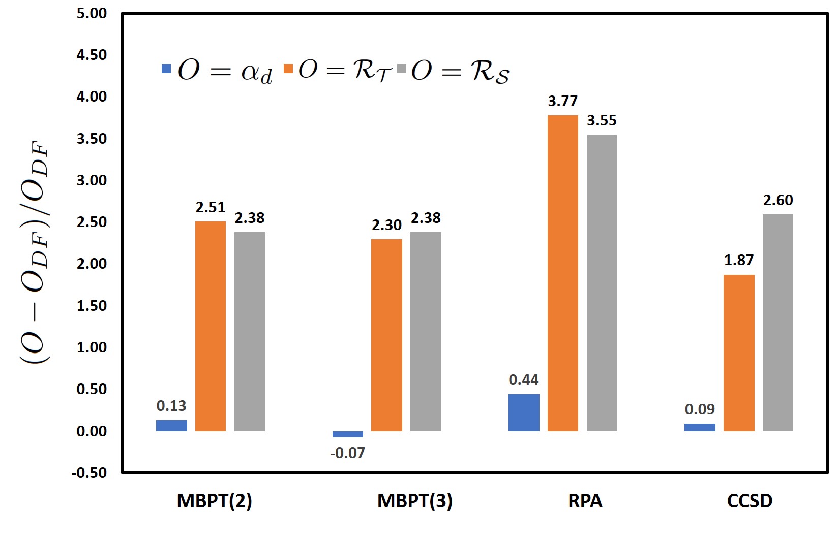
Figure 1: Comparison of electron correlation contributions to $\alpha_{d}$, ${\cal R_{T}}$, and ${\cal R_{S}}$ in ¹⁷¹Yb at different levels of approximations in the many-body methods with respect to the DHF results. No scaling has been maintained in the X-axis, while results plotted in the Y-axis are unit-less.

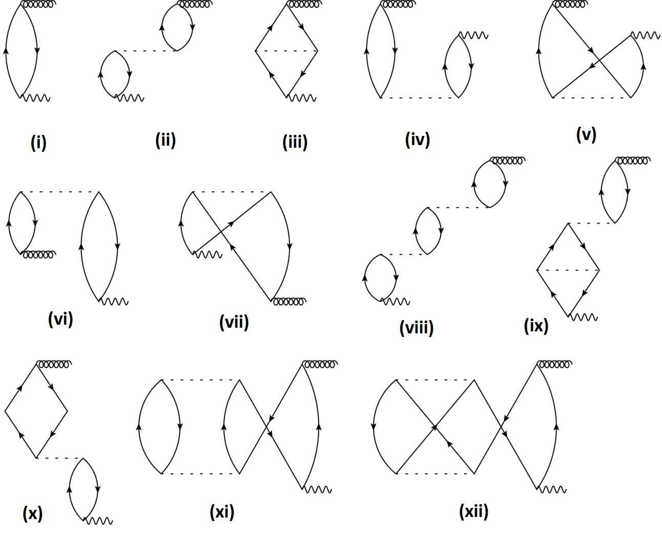
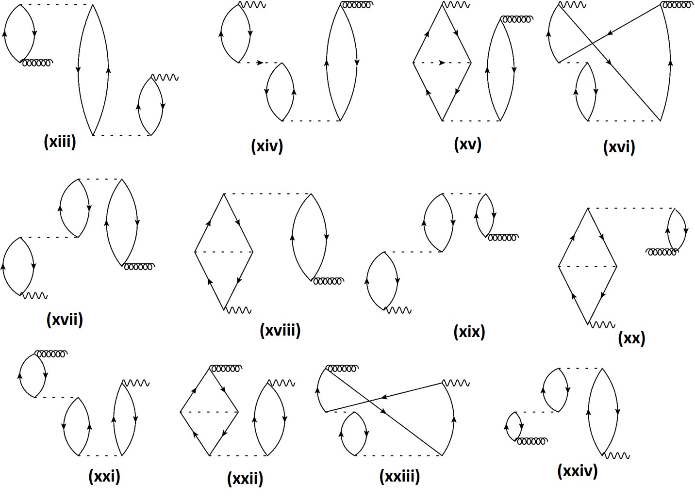
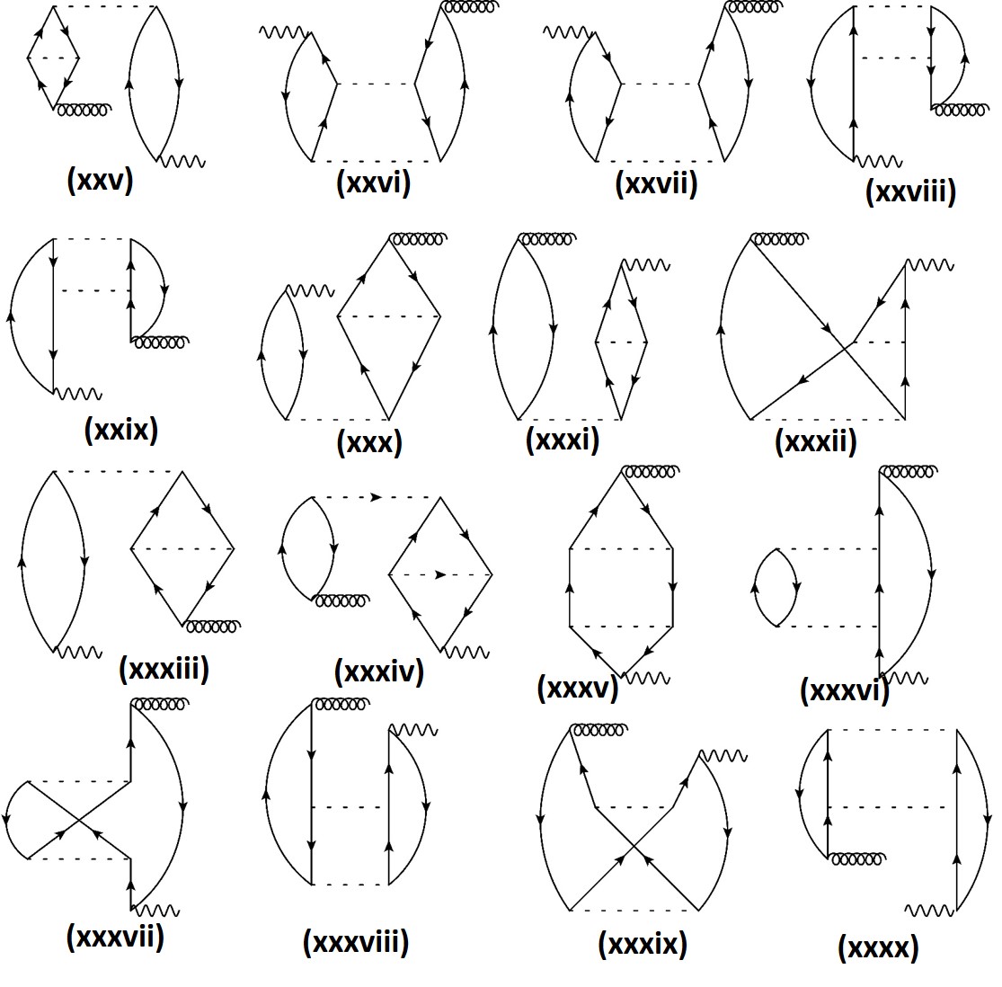
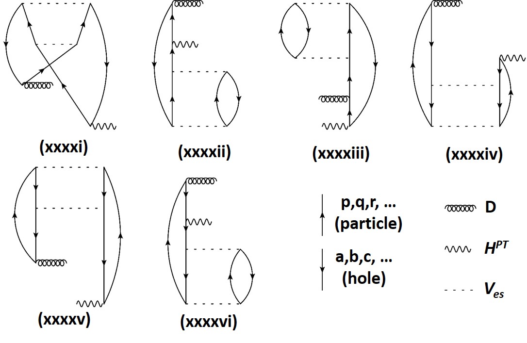
Figure 2: Important Goldstone diagrams belonging to the MBPT(3) method. Diagram (i) and diagrams up to (vii) correspond to the DHF and MBPT(2) methods, respectively. Operators appearing from right to left in Eqs. (29) and (30) are shown from bottom to top. Lines with arrows up and down represent for the virtual and core orbitals, respectively. Symbols for different operators are shown at the end.

Table 2: Explicit contributions to $\alpha_{d}$, ${\cal R_{T}}$, and ${\cal R_{S}}$ in units of $ea_{0}^{3}$, $\times 10^{-20}\langle\sigma\rangle|e|cm$ and $\times 10^{-17}[1/|e|fm^{3}]|e|cm$, respectively, from some of the important Goldstone diagrams of the MBPT(3) method. First one and along this the next six give DHF and MBPT(2) contributions, respectively.

Diagrams	$\alpha_{d}$	${\cal R_{T}}$	${\cal R_{S}}$
Fig. 2(i)	124.50	$-0.71$	$-0.42$
Fig. 2(ii)	$-46.95$	$-0.02$	$-0.01$
Fig. 2(iii)	92.82	$-1.29$	$-0.72$
Fig. 2(iv)	$-23.47$	$-0.41$	$-0.23$
Fig. 2(v)	8.91	$-0.29$	$-0.18$
Fig. 2(vi)	$-23.47$	0.39	0.22
Fig. 2(vii)	8.91	$-0.15$	$-0.08$
Fig. 2(viii)	25.03	0.16	0.09
Fig. 2(ix)	$-35.26$	0.51	0.28
Fig. 2(x)	$-35.26$	0.03	0.02
Fig. 2(xi)	$-31.05$	0.42	0.23
Fig. 2(xii)	9.07	$-0.11$	$-0.06$
Fig. 2(xiii)	5.11	0.13	0.07
Fig. 2(xiv)	7.69	0.26	0.14
Fig. 2(xv)	$-9.09$	0.04	0.03
Fig. 2(xvi)	$-2.25$	0.10	0.06
Fig. 2(xvii)	6.49	$-0.12$	$-0.07$
Fig. 2(xviii)	$-8.15$	0.13	0.07
Fig. 2(xix)	10.85	0.03	0.02
Fig. 2(xx)	$-18.02$	0.33	0.18
Fig. 2(xxi)	6.49	$-0.12$	$-0.07$
Fig. 2(xxii)	$-8.15$	0.12	0.07
Fig. 2(xxiii)	$-2.22$	0.10	0.06
Fig. 2(xxiv)	7.69	$-0.15$	$-0.08$
Fig. 2(xxv)	$-9.09$	0.16	0.08
Fig. 2(xxvi)	$-8.06$	0.14	0.07
Fig. 2(xxvii)	$-8.00$	0.12	0.06
Fig. 2(xxviii)	$-8.09$	0.14	0.08
Fig. 2(xxix)	$-8.12$	0.13	0.07
Fig. 2(xxx)	$-8.15$	0.12	0.07
Fig. 2(xxxi)	$-9.09$	0.04	0.03
Fig. 2(xxxii)	3.59	$-0.11$	$-0.07$
Fig. 2(xxxiii)	$-9.09$	0.16	0.08
Fig. 2(xxxiv)	$-8.18$	0.13	0.07
Fig. 2(xxxv)	70.93	$-1.24$	$-0.67$
Fig. 2(xxxvi)	15.72	$-0.43$	$-0.23$
Fig. 2(xxxvii)	$-3.84$	0.10	0.06
Fig. 2(xxxviii)	11.83	$-0.17$	$-0.10$
Fig. 2(xxxix)	5.38	$-0.11$	$-0.07$
Fig. 2(xxxx)	11.83	$-0.20$	$-0.11$
Fig. 2(xxxxi)	5.38	$-0.09$	$-0.05$
Fig. 2(xxxxii)	$-11.67$	$-0.25$	$-0.14$
Fig. 2(xxxxiii)	$-11.67$	$-0.04$	$-0.02$
Fig. 2(xxxxiv)	8.91	$-0.11$	$-0.06$
Fig. 2(xxxxv)	8.91	$-0.14$	$-0.07$
Fig. 2(xxxxvi)	$-0.19$	$-0.10$	$-0.06$

In Table 1, we present $\alpha_{d}$ and ${\cal R}$ values due to both the T-PT and NSM interactions in ¹⁷¹Yb by means of the earlier discussed many-body methods and compare them with the previously reported results dzuba7 ; dzuba9 ; dzuba2 ; latha ; radziute . For convenience, we denote ${\cal R}$ values due to the T-PT and NSM interactions as ${\cal R_{T}}$ and ${\cal R_{S}}$, respectively. As can be seen, the DHF value of $\alpha_{d}$ and the CCSD result differ marginally giving an impression that the roles of the electron correlation effects in the evaluation of atomic wave functions in this atom are not very strong. However, analyzing results for this quantity from the MBPT(2), MBPT(3), and RPA methods indicate a different scenario. The MBPT(2) method gives a larger value, while the MBPT(3) method gives a lower value of $\alpha_{d}$ from the DHF method. The all order RPA method gives a very large value than all these methods and the all order CCSD method brings down this value drastically. It can be noted that the MBPT(2) method posses all the lowest order core-polarization effects and the MBPT(3) method accounts for the lowest order correlation effects that do not belong to the core-polarization effects, which are discussed elaborately below. Significant differences between the $\alpha_{d}$ values from the MBPT(2) and MBPT(3) methods suggest substantial contributions from these other than core-polarization effects and with the opposite sign than the core-polarization contributions. In the all order level, differences between the RPA and CCSD results imply the net contributions from the other than core-polarization effects. A preliminary experimental result on $\alpha_{d}$ of the ground state of Yb has been reported with large uncertainty as 142(36) a.u. miller . However, many calculations on this quantities are carried out employing variants of many-body methods porsev ; zhang ; bksahoo ; dzuba ; safronova . Most of these calculations are not consistent owing to large electron correlation effects associated with this atom. We had also obtained earlier this value using the CCSD method and was reported as 144.59(5.64) a.u. bksahoo , considering only the linear terms of $\overline{D}^{(0)}$ in Eq. (32). We find inclusion of contributions from the non-linear terms reduces this value because of which we give a slightly smaller value here. Nevertheless, the present result is in close agreement with most of the theoretical values and also with the central value of the reported experimental result. From this, we can hope that our CCSD method can also estimate the ${\cal R}$ values with reasonable accuracies.

Table 3: Contributions to $\alpha_{d}$, ${\cal R_{T}}$, and ${\cal R_{S}}$ in units of $ea_{0}^{3}$, $\times 10^{-20}\langle\sigma\rangle|e|cm$ and $\times 10^{-17}[1/|e|fm^{3}]|e|cm$, respectively, from various CCSD terms (hermitian conjugate terms are included).

CCSD term	$\alpha_{d}$	${\cal R_{T}}$	${\cal R_{S}}$
$DT_{1}^{(1)}$	160.55	$-2.70$	$-1.87$
$T_{1}^{(0)\dagger}DT_{1}^{(1)}$	$-11.58$	$-0.04$	$-0.01$
$T_{2}^{(0)\dagger}DT_{1}^{(1)}$	$-19.62$	0.68	0.41
$T_{1}^{(0)\dagger}DT_{2}^{(1)}$	1.06	$-0.03$	0.02
$T_{2}^{(0)\dagger}DT_{2}^{(1)}$	9.05	$-0.01$	$-0.10$
Higher	$-3.96$	0.06	0.04

Though both the rank and parity of the E1 operator are same with the considered P,T-odd interaction operators, it can be clearly seen from Table 1 that the trends of electron correlation effects in the evaluation of the $\alpha_{d}$ and ${\cal R}$ values are completely different in these properties. The CCSD results for ${\cal R}$ are almost three times larger than their corresponding DHF values. However, the values obtained in the MBPT(2) method are larger than the CCSD results and the MBPT(3) values are smaller than the MBPT(2) results. The RPA method in these cases also give very large values as compared to the CCSD results. One can notice that the electron correlation effects in the evaluation of ${\cal R_{T}}$ and ${\cal R_{S}}$ are also somewhat different. The CCSD value for ${\cal R_{T}}$ is smaller than the MBPT values, while it is larger in case of the NSM interaction. In Fig. 1, we plot the $(O-O_{DF})/O_{DF}$ contributions to $\alpha_{d}$ and ${\cal R}$ values with $O$ representing values from different many-body methods, which highlight the amount of electron effects that are being accounted for in the evaluation of these quantities through the respective methods. This clearly demonstrates that the role electron correlation effects play vital roles in determining the ${\cal R}$ values more than the $\alpha_{d}$ result. Few earlier calculations on ${\cal R}$ are available using the configuration interaction (CI) angom , RPA dzuba7 ; dzuba2 ; dzuba9 ; latha , multi-configuration Dirac-Fock (MCDF) radziute and a combined CI and MBPT methods dzuba9 . Our RPA values agree with the RPA results of Dzuba et al dzuba7 ; dzuba2 , but differ slightly from the RPA values reported by Latha and Amjith latha . The CI, RPA and MCDF methods appear to overestimate the ${\cal R}$ values than the CCSD method. Similar trends of the correlation effects were also observed earlier in ¹⁹⁹Hg yashpal3 ; sahoo1 and in ²²⁵Ra yashpal4 . This clearly demands for employing a potential many-body method to evaluate the ${\cal R}$ values with the reasonable accuracy so that they can be combined with the future experimental result of the ¹⁷¹Yb atom to infer more reliable limits on the $C_{T}$ and $S$ values.

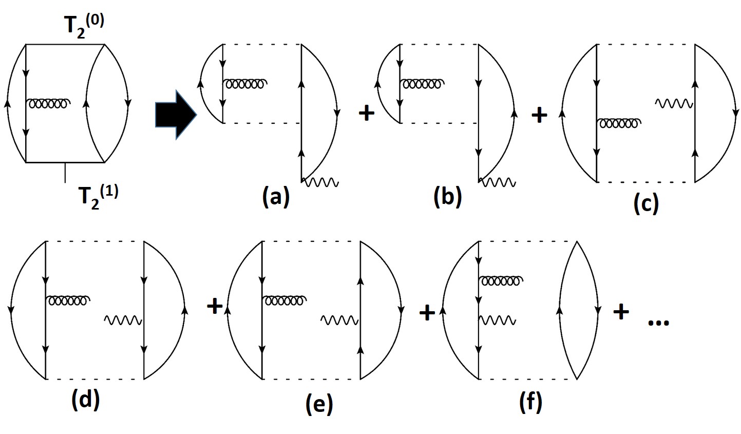
Figure 3: Breakdown of one of the all order diagrams representing the $T_{2}^{(0)\dagger}DT_{2}^{(1)}$ term is shown explicitly for the comprehensive understanding of how other than the core-polarization effects are accounted for through the CCSD method in the evaluation of the $\alpha_{d}$ and ${\cal R}$ values.

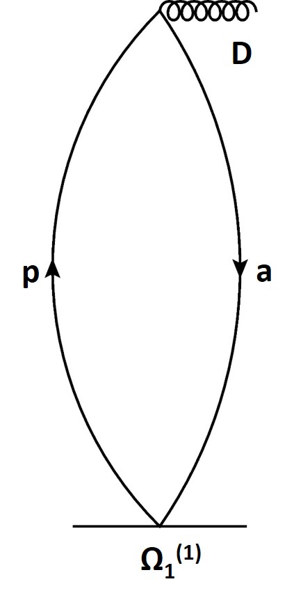
Figure 4: The Goldstone diagram depicting singly excitation contributions to $\alpha_{d}$ and ${\cal R}$ by exciting a core orbital “a” to a virtual orbital “p” through the $\Omega^{(1)}$ operator. Here $\Omega^{(1)}$ represents for the first order perturbed operator in the DHF, MBPT(2) and RPA methods and the $T_{1}^{(1)}$ operator of the CCSD method.

After presenting the final results from various many-body methods, we now intend to analyze the roles of the electron correlation effects in the evaluation of the $\alpha_{d}$ and ${\cal R}$ values through various Goldstone diagrams of the MBPT, RPA and CCSD methods. In Fig. 2, we show some of the important diagrams belonging to the MBPT(3) method. There are more than 200 diagrams appear in the MBPT(3) method, but we present here contributions only from the selective diagrams that contribute substantially. The first diagram of Fig. 2 represents for the DHF method and diagrams up to Fig. 2(vii) correspond to the MBPT(2) method. Individual contribution from these diagrams to $\alpha_{d}$ and ${\cal R}$ are given in Table 2. Some of the non-quoted diagrams also contribute in the similar orders with slightly smaller values, but their contributions are not mentioned explicitly here to avoid a very long table. As can be seen from this table, magnitudes and signs of the contributions from various diagrams to $\alpha_{d}$ and ${\cal R}$ with respect to their respective final values exhibit different trends. Contributions from some diagrams to $\alpha_{d}$ are large, while they contribute tinier to ${\cal R}$. It is also found that some of the individual diagrams contribute as large as three-fourth of the total value to $\alpha_{d}$. Certain third order perturbative diagrams also contribute more than the second order diagrams to this property. Diagrams shown as Fig. 2(xi), (xii), (xxvi), (xxvii), (xxix), (xxxvi), (xxxxii), (xxxxiii), (xxxxiv), (xxxxv), (xxxxvi) etc. are some of the dominantly contributing MBPT(3) diagrams that represent for other than the core-polarization effects. These diagrams are solely responsible for bringing down the MBPT(3) values from the results obtained using the MBPT(2) method. They do not appear through the all order RPA method but appear in the CCSD method to all orders. This is the main reason why the CCSD results are found to be much smaller than the RPA values as quoted in Table 1. Comparing contributions to the ${\cal R}$ values from the T-PT and NSM interactions, we find they maintain a scaling among the contributions from each diagram. Contributions to the T-PT result are about two times larger than the NSM contributions for the individual diagram. In fact, some of the correlation contributions to $\alpha_{d}$ are found to have opposite sign than its DHF value, hence canceling out a large part of the correlation contributions to give the smaller net value. Contrary, the dominant contributions from the MBPT method to ${\cal R}$ have the same sign with their DHF values from the respective P,T-odd interactions. This is why enhancement in the ${\cal R}$ values from their DHF values are found to be much larger than the $\alpha_{d}$ result. It is also found that other than the core-polarization contributions are proportionally larger in the determination of the ${\cal R}$ values than the $\alpha_{d}$ result.

Table 4: Contribution from various atomic orbitals to $\alpha_{d}$, ${\cal R_{T}}$, and ${\cal R_{S}}$ in units of $ea_{0}^{3}$, $\times 10^{-20}\langle\sigma\rangle|e|cm$ and $\times 10^{-17}[1/|e|fm^{3}]|e|cm$, respectively, through dominantly contributing singly excitations represented by Fig. 4. Values that are smaller in magnitudes are approximated to zero (mentioned as $\sim 0.0)$ and those marked in bold fonts highlight changes in the trends of the results from the DHF method after incorporating electron correlation effects through different many-body methods. Contributions from the $6s$ and $p_{3/2}$ orbitals are quoted within two lines to demonstrate how they behave differently in the evaluation of the $\alpha_{d}$ and ${\cal R}$ values using the considered methods.

Occupied	Virtual	$\alpha_{d}$				${\cal R_{T}}$				${\cal R_{S}}$
$a$	$p$	DHF	MBPT(2)	RPA	$DT_{1}^{(1)}$	DHF	MBPT(2)	RPA	$DT_{1}^{(1)}$	DHF	MBPT(2)	RPA	$DT_{1}^{(1)}$
$4s$	$11p_{1/2}$	$\sim 0.0$	$\sim 0.0$	$\sim 0.0$	$\sim 0.0$	0.02	$-0.07$	0.03	0.03	0.01	$-0.02$	0.01	0.01
$3s$	$12p_{1/2}$	$\sim 0.0$	$\sim 0.0$	$\sim 0.0$	$\sim 0.0$	0.02	$-0.04$	0.02	0.02	0.01	$-0.01$	0.01	0.01
$4s$	$12p_{1/2}$	$\sim 0.0$	$\sim 0.0$	$\sim 0.0$	$\sim 0.0$	0.05	$-0.14$	0.05	0.05	0.01	$-0.03$	0.01	0.01
$5s$	$10p_{1/2}$	$\sim 0.0$	$\sim 0.0$	$\sim 0.0$	$\sim 0.0$	0.04	0.09	0.05	0.05	0.01	0.02	0.01	0.01
$5s$	$11p_{1/2}$	$\sim 0.0$	$\sim 0.0$	$\sim 0.0$	$\sim 0.0$	0.07	0.01	0.08	0.08	0.02	$\sim 0.0$	0.02	0.02
$5s$	$12p_{1/2}$	$\sim 0.0$	$\sim 0.0$	$\sim 0.0$	$\sim 0.0$	0.02	$-0.06$	0.02	0.02	$\sim 0.0$	$-0.01$	0.01	0.01
$6s$	$6p_{1/2}$	9.38	12.39	15.97	11.84	$-0.22$	$-0.29$	$-0.78$	$-0.76$	$-0.05$	$-0.07$	$-0.18$	$-0.16$
$6s$	$7p_{1/2}$	22.54	28.94	37.35	29.90	$-0.69$	$-0.88$	$-{\bf 2.32}$	$-{\bf 2.29}$	$-0.17$	$-0.21$	$-{\bf 0.54}$	$-{\bf 0.49}$
$6s$	$8p_{1/2}$	7.95	8.80	11.37	12.09	$-0.52$	$-0.57$	$-{\bf 1.53}$	$-{\bf 1.59}$	$-0.12$	$-0.14$	$-{\bf 0.37}$	$-{\bf 0.35}$
$6s$	$9p_{1/2}$	0.20	0.20	0.04	0.36	$-0.12$	0.05	$-0.27$	$-0.29$	$-0.03$	0.01	$-0.07$	$-0.07$
$6s$	$10p_{1/2}$	$\sim 0.0$	$\sim 0.0$	$\sim 0.0$	$\sim 0.0$	0.02	0.11	0.03	0.03	$\sim 0.0$	0.03	0.01	0.01
$6s$	$6p_{3/2}$	14.01	18.57	23.44	17.54	$\sim 0.0$	$\sim 0.0$	0.05	0.19	$-0.05$	$-0.07$	$-0.16$	$-0.13$
$6s$	$7p_{3/2}$	43.44	55.96	70.39	57.35	$\sim 0.0$	$\sim 0.0$	0.17	0.71	$-0.21$	$-0.27$	$-{\bf 0.63}$	$-{\bf 0.53}$
$6s$	$8p_{3/2}$	18.73	20.99	25.86	28.03	$\sim 0.0$	$\sim 0.0$	0.06	0.48	$-0.21$	$-0.21$	$-{\bf 0.52}$	$-{\bf 0.48}$
$5p_{1/2}$	$8s$	$\sim 0.0$	$\sim 0.0$	$\sim 0.0$	$\sim 0.0$	0.02	$\sim 0.0$	0.02	0.02	$\sim 0.0$	$\sim 0.0$	0.01	$\sim 0.0$
$5p_{1/2}$	$9s$	0.03	$\sim 0.0$	$-0.03$	$\sim 0.0$	0.09	$-0.02$	0.13	0.11	0.02	$\sim 0.0$	0.03	0.03
$4p_{1/2}$	$10s$	$\sim 0.0$	$\sim 0.0$	$\sim 0.0$	$\sim 0.0$	0.01	$-0.02$	0.01	0.01	$\sim 0.0$	$-0.01$	$\sim 0.0$	$\sim 0.0$
$5p_{1/2}$	$10s$	0.03	$-0.01$	$-0.04$	$\sim 0.0$	0.19	$-0.09$	0.26	0.24	0.05	$-0.02$	0.07	0.06
$4p_{1/2}$	$11s$	$\sim 0.0$	$\sim 0.0$	$\sim 0.0$	$\sim 0.0$	0.04	$-0.12$	0.04	0.04	0.01	$-0.03$	0.01	0.01
$5p_{1/2}$	$11s$	$\sim 0.0$	$\sim 0.0$	$\sim 0.0$	$\sim 0.0$	0.09	$-0.12$	0.10	0.10	0.02	$-0.03$	0.03	0.02
$3p_{1/2}$	$12s$	$\sim 0.0$	$\sim 0.0$	$\sim 0.0$	$\sim 0.0$	0.01	$-0.02$	0.02	0.02	$\sim 0.0$	$-0.01$	$\sim 0.0$	$\sim 0.0$
$4p_{1/2}$	$12s$	$\sim 0.0$	$\sim 0.0$	$\sim 0.0$	$\sim 0.0$	0.03	$-0.08$	0.03	0.03	0.01	$-0.02$	0.01	0.01
$5p_{3/2}$	$8s$	0.03	$\sim 0.0$	$-0.03$	0.01	$\sim 0.0$	$\sim 0.0$	$\sim 0.0$	$\sim 0.0$	0.01	$\sim 0.0$	0.01	0.01
$5p_{3/2}$	$9s$	0.11	$-0.03$	$-0.13$	0.02	$\sim 0.0$	$\sim 0.0$	0.02	0.01	0.04	$-0.01$	0.07	0.06
$4p_{3/2}$	$10s$	$\sim 0.0$	$\sim 0.0$	$\sim 0.0$	$\sim 0.0$	$\sim 0.0$	$\sim 0.0$	$\sim 0.0$	$\sim 0.0$	0.01	$-0.01$	0.01	0.01
$5p_{3/2}$	$10s$	0.10	$-0.06$	$-0.13$	$\sim 0.0$	$\sim 0.0$	$\sim 0.0$	0.03	0.02	0.08	$-0.05$	0.12	0.11
$4p_{3/2}$	$11s$	$\sim 0.0$	$\sim 0.0$	$\sim 0.0$	$\sim 0.0$	$\sim 0.0$	$\sim 0.0$	$\sim 0.0$	$\sim 0.0$	0.02	$-0.05$	0.01	0.02
$5p_{3/2}$	$11s$	$\sim 0.0$	$-0.01$	$\sim 0.0$	$\sim 0.0$	$\sim 0.0$	$\sim 0.0$	$\sim 0.0$	$\sim 0.0$	0.03	$-0.05$	0.03	0.04
$3p_{3/2}$	$12s$	$\sim 0.0$	$\sim 0.0$	$\sim 0.0$	$\sim 0.0$	$\sim 0.0$	$\sim 0.0$	$\sim 0.0$	$\sim 0.0$	0.01	$-0.01$	$\sim 0.0$	0.01
$4p_{3/2}$	$12s$	$\sim 0.0$	$\sim 0.0$	$\sim 0.0$	$\sim 0.0$	$\sim 0.0$	$\sim 0.0$	$\sim 0.0$	$\sim 0.0$	0.01	$-0.03$	0.01	0.01
$5p_{3/2}$	$12s$	$\sim 0.0$	$\sim 0.0$	$\sim 0.0$	$\sim 0.0$	$\sim 0.0$	$\sim 0.0$	$\sim 0.0$	$\sim 0.0$	$\sim 0.0$	$-0.01$	$\sim 0.0$	$\sim 0.0$

In Table 3, we present contributions from the individual CCSD terms. This shows the dominant contributions come from the $DT_{1}^{(1)}$ term followed by $T_{2}^{(0)\dagger}DT_{1}^{(1)}$. Contribution from $T_{1}^{(0)\dagger}DT_{1}^{(1)}$ to $\alpha_{d}$ is also quite large, however its contributions to ${\cal R}$ are very small. It can be noticed from Fig. 1 that contributions from most of these diagrams from the MBPT(3) method are accounted for in the $DT_{1}^{(1)}$ term through the RCC formulation and the rest arise through the $T_{2}^{(0)\dagger}DT_{1}^{(1)}$ term. This is the reason why $DT_{1}^{(1)}$ and $T_{2}^{(0)\dagger}DT_{1}^{(1)}$ terms have major shares to the CCSD results as demonstrated in Table 3. In addition to the above, contributions coming through $T_{1}^{(0)\dagger}DT_{1}^{(1)}$ are also from the singly excitations in the configuration space and offer significant shares to the final results. It can be noticed from the above table that a substantial amount of contributions also come through the $T_{2}^{(0)\dagger}DT_{2}^{(1)}$ term. Breakdown of one of its diagrams into some of the MBPT(3) diagrams are shown in Fig. 3. As seen from this figure, all the contributions arising through the $T_{2}^{(0)\dagger}DT_{2}^{(1)}$ term are due to other than the core-polarization effects and they are important in determining the $\alpha_{d}$ value, while they contribute relatively smaller in the evaluation of the ${\cal R}$ values. These MBPT(3) diagrams were not shown explicitly in Fig. 1 as each of these diagrams contribute small, but they add up to a sizable amount in the CCSD method. In the above table, we also quote contributions from the remaining terms of the CCSD method as “Higher”, because they correspond to higher order correlation effects and arise through the non-linear terms such as the $T_{1}^{(0)\dagger}DT_{1}^{(0)}T_{1}^{(1)}$, $T_{2}^{(0)\dagger}DT_{2}^{(0)}T_{1}^{(1)}$, etc. terms. Most of these contributions are due to other than the core-polarization effects.

The Goldstone diagram depicting the $D\Omega^{(1)}$ term with the approximation for $\Omega^{(1)}$ as the first order perturbed operator in the DHF, MBPT(2) and RPA methods and the $T_{1}^{(1)}$ operator of the CCSD method is shown in Fig. 4. This represents the dominantly contributing singly excited configurations, which we have represented replacing a core orbital (a), denoted with a line pointing down arrow, by a virtual orbital (p), denoted with a line with upward arrow, at various levels of approximations. Contributions from this diagram at the DHF, MBPT(2), RPA and CCSD level are listed in Table 4 only from the large contributing orbitals. As can be seen from this table, contributions from various orbitals to $\alpha_{d}$ and ${\cal R}$ values are different. In the determination of $\alpha_{d}$, only the $6s$ and $p_{1/2,3/2}$ orbitals play all the roles. This trend also shows why and how the RPA result for $\alpha_{d}$ becomes very large, particularly through the $6s-7p_{3/2}$ orbitals. It exhibits that the core-polarization effects are changing contributions from these orbitals very strongly at the MBPT(2) and RPA level of approximations, while other types of correlation effects coming through the $DT_{1}^{(1)}$ RCC term revamp these orbitals further to bring these values down. It can also be seen that the $6s-p_{3/2}$ orbitals contribute more than the $6s-p_{1/2}$ orbitals to this quantity. Comparison with the $\alpha_{d}$ results, the correlation effects affect more strongly to the atomic orbitals in the evaluation of the ${\cal R}$ values. Again, the $6s-p_{1/2}$ orbitals contribute predominantly in the evaluation of ${\cal R}$ than the $6s-p_{3/2}$ orbitals. In fact, contributions from the $6s-p_{3/2}$ to these quantities at the DHF values are negligibly small and other than the core-polarization effects through the $DT_{1}^{(1)}$ RCC term modified these orbitals drastically to give a quite significant contributions to the final results. To highlight the same, results only from the $6s-p_{3/2}$ orbitals are put in between two lines of the above table. It can also be noticed that the $6s$ and $p_{1/2,3/2}$ orbitals contribute differently to the ${\cal R_{T}}$ and ${\cal R_{S}}$ values at various levels of approximations in the many-body methods. In contrast to the $\alpha_{d}$ value, some of the high-lying orbitals also contribute substantially to these quantities as these continuum have large overlap over the nuclear region. We have marked in bold fonts to some of the quoted contributions from few specific orbitals to bring into notice how the electron correlation effects modifies these orbitals unusually large in ¹⁷¹Yb for studying atomic properties. This implies that it is important to consider a potential many-body method to determine the ${\cal R}$ values in this atom. It also suggests testing accuracies of the $\alpha_{d}$ value cannot justify accuracies of the ${\cal R}$ values absolutely, but it can only assure validity of the calculations to some extent.

V Conclusion

Roles of electron correlation effects in the determination of dipole polarizability and electric dipole moment due to parity and time reversal symmetry violations considering the tensor-pseudotensor interactions between the electrons with the nucleus and electrons with the nuclear Schiff moment in the ¹⁷¹Yb atom are analyzed. For this purpose, relativistic many-body methods over the Dirac-Hartree-Fock wave function at the approximations of the second and third order many-body perturbation theories, random phase approximation and coupled-cluster method with singles and doubles excitations are employed. Contributions from the core-polarization effects and other possible correlation interactions are investigated categorically from the differences of the random phase approximation and coupled-cluster calculations. To fathom the origin of these differences, contributions in terms of the important Goldstone diagrams appearing through the second-order and third-order perturbative methods are given. Moreover, contributions from different orbitals at various levels of approximations in the many-body methods listed for the comprehensive understanding of propagation of the electron correlation effects in the above atom through these orbitals to the considered properties that have distinct radial behaviors. This suggests that accuracies in the calculated electric dipole moments in atoms cannot be really determined from the dipole polarizability calculations. On the grounds of physical effects that are being embodied in the calculations, the values obtained employing our coupled-cluster method are more accurate and they can be used to infer reliable limits on the tensor-pseudotensor coupling constant between the electrons and nucleus and nuclear Schiff moment of the ¹⁷¹Yb atom when its experiment comes to fruition.

References

- (1) I. B. Khriplovich and S. K. Lamoreaux, CP Violation Without Strangeness (Springer, Berlin, 1997).
- (2) M. Pospelov and A. Ritz, Ann. Phys. (N.Y.) 318, 119 (2005).
- (3) V. A. Dzuba and V. V. Flambaum, Int. J. Mod. Phys. E 21, 1230010 (2012).
- (4) N. Yamanaka, B. K. Sahoo, N. Yoshinaga, T. Sato, K. Asahi, and B. P. Das, Eur. Phys. J. A 53, 54 (2017).
- (5) S. A. Murthy, D. Krause, Jr., Z. L. Li, and L. R. Hunter Phys. Rev. Lett. 63, 965 (1989).
- (6) C. Chin, V. Leiber, V. Vuletić, A. J. Kerman, and S. Chu Phys. Rev. A 63, 033401 (2001).
- (7) B. C. Regan et al., Phys. Rev. Lett. 88, 071805 (2002).
- (8) M. A. Rosenberry and T. E. Chupp Phys. Rev. Lett. 86, 22 (2001).
- (9) W. C. Griffith, M. D. Swallows, T. H. Loftus, M. V. Romalis, B. R. Heckel, and E. N. Fortson Phys. Rev. Lett. 102, 101601 (2009).
- (10) B. Graner, Y. Chen ((陳宜)), E. G. Lindahl, and B. R. Heckel Phys. Rev. Lett. 116, 161601 (2016).
- (11) R. H. Parker et al. Phys. Rev. Lett. 114, 233002 (2015).
- (12) J. J. Hudson et al, Nature 473, 493 (2011).
- (13) J. Baron et al, Science 343, 269 (2014).
- (14) M. Dine and A. Kusenko, Rev. Mod. Phys. 76, 1 (2003).
- (15) L. Canetti, M. Drewes and M. Shaposhnikov, New J. Phys. 14, 095012 (2012).
- (16) T. Inoue et al., Hyperfine Interactions (Springer Netherlands) 220, 59 (2013).
- (17) P. Fierlinger et al., Cluster of Excellence for Fundamental Physics, Technische UniversitätM ünchen, http://www.universecluster.de/fierlinger/xedm.html
- (18) U. Schmidt et al., Collaboration of the Helium Xenon EDM Experiment, Physikalisches Institut, University of Heidelberg, http://www.physi.uniheidelberg.de/Forschung/ANP/XenonEDM/Team.
- (19) A. Yoshimi et al., Phys. Lett. A 304, 13 (2002).
- (20) N. Auerbach, V. V. Flambaum, and V. Spevak, Phys. Rev. Lett. 76, 4316 (1996).
- (21) E. T. Rand et al., J. Phys.: Conf. Series 312 102013 (2011).
- (22) Tardiff et al., Hyperfine Interactions 225, 197 (2014).
- (23) Y. Singh, B. K. Sahoo and B. P. Das, Phys. Rev. A 89, 030502(R) (2014).
- (24) B. K. Sahoo, Y. Singh and B. P. Das, Phys. Rev. A 90, 050501(R) (2014).
- (25) Y. Singh and B. K. Sahoo, Phys. Rev. A 91, 030501(R) (2015).
- (26) B. K. Sahoo, Phys. Rev. D 95, 013002 (2017).
- (27) Y. Singh and B. K. Sahoo, Phys. Rev. A 92, 022502 (2015).
- (28) T. Xia, M. Dietrich, and Z.-T. Lu, EDM measurements on cold 225Ra and 171Yb atoms, K1.00026 Abstract, 48th Annual Meeting of the APS Division of Atomic, Molecular and Optical Physics, June 5–9, 2017 (Sacramento, California) USA.
- (29) Y. Takahashi, M. Fujimoto, T. Yabuzaki, A. D. Singh, M. K. Samal, and B.P.Das, Electric Dipole Moment of Atomic Ytterbium by Laser Cooling and Trapping, Proceedings of CP Violation and its Origin, edited by K. Hagiwara, p. 259, KEK Report, Tsukuba, (1997).
- (30) M.V. Romalis and E.N. Fortson, Phys. Rev. A 59, 4547 (1999).
- (31) V. Natarajan Eur. Phys. J. D 32, 33-38 (2005).
- (32) T. Takano, M. Fuyama, H. Yamamoto, and Y. Takahashi, poster presented at 17th International Spin Physics Symposium, Oct. 2-7 2006, Kyoto.
- (33) A. D. Singh, B. P. Das, W. F. Perger, M. K. Samal and K. P. Geetha, J. Phys. B 34, 3089 (2001).
- (34) V. A. Dzuba, V. V. Flambaum, J. S. M. Ginges and M. G. Kozlov, Phys. Rev. A 66, 012111 (2002).
- (35) V. A. Dzuba, V. V. Flambaum, and J. S. M. Ginges, Phys. Rev. A 76, 034501 (2007).
- (36) V. A. Dzuba, V. V. Flambaum and S. G. Porsev, Phys. Rev. A 80, 032120 (2009).
- (37) K. V. P. Latha and P. R. Amjith, Phys. Rev. A 87, 022509 (2013).
- (38) S. M. Barr, Phys. Rev. D 45, 4148 (1992).
- (39) A.-M. Maartensson-Pendrill, Phys. Rev. Lett. 54, 1153 (1985).
- (40) V. V. Flambaum and J. S. M. Ginges, Phys. Rev. A 65, 032113 (2002).
- (41) W. C. Haxton and E. M. Henley, Phys. Rev. Lett. 51, 1937 (1983).
- (42) S. Ban, J. Dobaczewski, J. Engel and A. Shukla, Phys. Rev. C 82, 015501 (2010).
- (43) J. H. de Jesus and J. Engel, Phys. Rev. C 72, 045503 (2005).
- (44) J. Engel, M. J. Ramsey-Musolf, and U. van Kolck, Prog. Part. Nucl. Phys. 71, 21 (2013).
- (45) M. Pospelov, Phys. Lett. B 530, 123 (2002).
- (46) W. Dekens et al., JHEP, 1407, 069 (2014).
- (47) V. F. Dmitriev and R. A. Sen’kov, Phys. Rev. Lett. 91, 212303 (2003).
- (48) I. Lindgren and J.Morrison, Atomic Many-Body Theory, 2nd ed. (Springer-Verlag, Berlin, 1986).
- (49) Y. Singh, B. K. Sahoo and B. P. Das, Phys. Rev. A 88, 062504 (2013).
- (50) L. Radžiūté, G. Gaigalas, P. Jönsson, and J. Bieroń Phys. Rev. A 90, 012528 (2014).
- (51) T. M. Miller, CRC Handbook of Chemistry and Physics, 77th ed., edited by D. R. Lide (CRC Press, Boca Raton, FL, 1996).
- (52) S. G. Porsev and A. Derevianko, Phys. Rev. A 74, 020502(R) (2006).
- (53) P. Zhang and A. Dalgarno, J. Phys. Chem. A 111, 12471 (2007).
- (54) B. K. Sahoo and B. P. Das, Phys. Rev. A 77, 062516 (2008).
- (55) M. S. Safronova, S. G. Porsev, and Charles W. Clark, Phys. Rev. Lett. 109, 230802 (2012).