On the spectrum and polarization of magnetar flare emission

Abstract

Bursts and flares are among the distinctive observational manifestations of magnetars, isolated neutron stars endowed with an ultra-strong magnetic field ($B\approx 10^{14}$–$10^{15}$ G). It is believed that these events arise in a hot electron-positron plasma which remains trapped within the closed magnetic field lines. We developed a simple radiative transfer model to simulate magnetar flare emission in the case of a steady trapped fireball. After dividing the fireball surface in a number of plane-parallel slabs, the local spectral and polarization properties are obtained integrating the radiative transfer equations for the two normal modes. We assume that magnetic Thomson scattering is the dominant source of opacity, and neglect contributions from second-order radiative processes, although double-Compton scattering is accounted for in establishing local thermal equilibrium in the fireball atmospheric layers. The observed spectral and polarization properties as measured by a distant observer are obtained summing the contributions from the patches which are visible for a given viewing geometry by means of a ray-tracing code. The spectra we obtained in the $1$–$100$ keV energy range are thermal and can be described in terms of the superposition of two blackbodies. The blackbody temperature and the emitting area ratio are in broad agreement with the available observations. The predicted linear polarization degree is in general greater than $80\%$ over the entire energy range and should be easily detectable by new-generation X-ray polarimeters, like IXPE, XIPE and eXTP.

1 Introduction

Soft gamma repeaters (SGRs) and anomalous X-ray pulsars (AXPs) are regarded as the observational manifestations of the same class of neutron stars (NSs), aka the magnetars, for which the long measured spin periods ($P\approx 2$–$12$ s) and large period derivatives ($\dot{P}\approx 10^{-13}$–$10^{-10}$ ss^-1) lead to a huge value of the dipole magnetic field, $B\approx 10^{14}$–$10^{15}$ G, well above those of other NS classes (see Turolla et al., 2015; Mereghetti, 2008, for reviews). Magnetars show an X-ray persistent emission with luminosity in the range $10^{33}$–$10^{36}$ ergs^-1, some orders of magnitude greater than the spin-down luminosity $\dot{E}_{\mathrm{rot}}$ inferred from $P$ and $\dot{P}$. One of the most distinctive properties of SGRs/AXPs is the emission of short ($\approx 10^{-2}$–$1$ s), energetic ($\approx 10^{36}$–$10^{41}$ erg) X-ray bursts and longer ($\approx 1$–$50$ s), even more energetic ($\approx 10^{41}$–$10^{43}$ erg) intermediate flares. Furthermore, three SGRs have been observed to emit also giant flares, the most powerful events ever observed from compact objects, characterized by a short ($\approx 0.1$–$1$ s) initial spike, followed by a long ($\approx 10^{2}$–$10^{3}$ s) pulsating tail modulated at the spin frequency of the star, with a total energy release $\approx 10^{44}$–$10^{47}$ erg.

According to the magnetar model, firstly developed by Duncan & Thompson (1992), magnetar activity is sustained by the magnetic energy stored in the huge (internal) magnetic field. The latter is believed to develop a large toroidal component (see e.g. Braithwaite, 2009; Perna & Pons, 2011), able to exert a strong magnetic stress on the conductive star crust. Contrary to what happens in “normal” NSs, where this force can be balanced by the rigidity of the crust, in the case of magnetars the internal stresses are strong enough to displace single surface elements (the so-called starquakes), owing to their ultra-strong fields. As a result, the external magnetic field acquires in turn a non-zero toroidal component, becoming twisted, and this makes possible for charged particles to fill the magnetosphere, streaming along the closed field lines Thompson et al. (2002); Nobili, Turolla & Zane (2008); Turolla et al. (2015).

The mechanisms that trigger magnetar bursting activity are still not completely clear. It has been proposed (see Lyutikov, 2003; Woods et al., 2005, see also Elenbass et al. 2016 for a discussion) that fast acceleration of magnetospheric particles, after spontaneous magnetic field reconnections, could be responsible for the enormous energy release and the light curves observed in particular kinds of SGR bursts. Thompson & Duncan (1995, 2001) suggested an alternative model to explain the giant flare trigger and emission mechanisms. According to them, an internal magnetic field instability induces large-amplitude oscillations in the magnetosphere, that convert, in turn, into a hot electron-positron plasma. While part of this plasma quickly escapes outwards in the initial phases, producing the hard initial peak of giant flares, another part remains trapped within the closed magnetic field lines, resulting in an optically-thick, photon-pair fireball. The long pulsating tail observed in these extreme events should be due indeed to the radiation coming from this confined, cooling region in the magnetosphere. The same paradigm can be also used to properly explain the shorter intermediate flares, which show as well a clearly detectable decay tail Olive et al. (2004); Feroci et al. (2004); Israel et al. (2008).

Although many efforts have been made in the last decades to explain the physics of magnetars, a detailed theoretical framework for modeling the spectral and polarization properties of the radiation emitted during magnetar flares does not yet exist. Spectral properties are difficult to investigate due to the rarity of intermediate/giant flares and the extremely small duration times of short bursts. On the other hand, as shown e.g. by Israel et al. (2008), the occurrence of batches of these events, during which a great number of single short bursts and intermediate flares can be emitted, could compensate for their short duration and provide enough statistics for a meaningful analysis. In the case of mangetars also polarimetry, besides spectral analysis, can be profitably used to characterize the observed radiation and identify its production mechanisms. In fact, in the presence of strong magnetic fields photons are expected to be highly polarized in two normal modes, the ordinary and the extraordinary modes. The radiative processes that take place in the magnetosphere generally influence the polarization pattern of the emitted radiation (see Mészáros, 1992; Nobili, Turolla & Zane, 2008). Moreover, for magnetic field intensities high enough, the photon polarization is modified also when they propagate in vacuo (the vacuum birefringence effect, see Heisemberg & Euler, 1936, see also Heyl & Shaviv 2002; Mignani et al. 2017 and references therein). This kind of analysis has not been possible so far, given that no instruments are available to perform polarization measurements in the X-rays. Nevertheless, new impetus was given in this field by new-generation instruments like IXPE (Weisskopf et al., 2013, recently approved for the NASA SMEX program and to be launched within 2020), XIPE (Soffitta, 2016, in the study phase of ESA M4 program) and eXTP Zhang et al. (2016), which promise to open a new window in X-ray astrophysics.

The problem of radiative transfer in a scattering medium in the presence of strong magnetic fields, as well as its possible applications to the spectra of SGR bursts, have been addressed by Lyubarsky (2002). Starting from the same theoretical framework as in Thompson & Duncan (1995, 2001), he calculated the spectra of radiation escaping from a plane-parallel slab of the pair fireball, in one dimensional approximation and assuming the star magnetic field parallel to the slab normal. More recently, Yang & Zhang (2015) have presented Montecarlo simulations to study the polarization properties of giant flare decay tail emission. They asssumed that the pair plasma produced during the magnetar flare remains trapped within a set of closed (dipolar) magnetic field lines and solved the radiative transport in a geometrically-thin, surface layer of the fireball, where magnetic Thomson scattering is the only source of opacity. According to the results of their simulations, radiation emitted during such events would be only mildly polarized, with maximum polarization degree in between $\approx 10$ and $30\%$ depending on the photon energy. The spectrum and polarization of magnetar flare radiation have been also studied by van Putten et al. (2016). While considering as well the effects of magnetic scattering on photons that propagate through a trapped fireball (modelled in a similar way as in Yang & Zhang 2015), they focused in particular on the radiation beaming driven by the presence of a mildly-relativistic, baryon-loaded outflow outside the fireball (predicted in the model by Thompson & Duncan, 1995, 2001), in order to describe consistently the observed pulse profiles and the expected evolution of a magnetar fireball. However, a detailed analysis of the spectral and polarization properties of the emitted radiation was outside the scope of their work.

In this paper we reconsider the problem of both the spectrum and polarization of the radiation emitted from a steady trapped fireball, providing simulations directly comparable with observations. As in Yang & Zhang (2015), we compute the photon transport in the surface layer of the fireball, following the approach by Lyubarsky (2002) and assuming magnetic Thomson scattering as the dominant source of opacity in the plasma. We neglect the contributions from second-order radiative processes, although the presence of double-Compton scattering is accounted for in establishing local thermal equilibrium in the fireball atmospheric layers. In particular, after dividing the fireball surface in a number of plane-parallel slabs, we obtain the local spectral and polarization properties integrating the radiative transfer equations for the two normal modes. The observed spectral and polarization properties as measured by a distant observer are obtained summing the contributions from the patches which are visible for a given viewing geometry by means of a ray-tracing code. Our results show that the simulated spectra in the $1$–$100$ keV energy range can be suitably described in terms of the superposition of two blackbody components, with temperatures and emitting area ratio in broad agreement with the observations available so far (see e.g. Israel et al., 2008; Olive et al., 2004; Feroci et al., 2004). Furthermore, the predicted polarization pattern significantly differs from those presented in previous works. In fact, the linear polarization degree turns out to be in general greater than $80\%$ over the entire energy range. Such a large degree of polarization should be easily detectable by new-generation X-ray polarimeters, allowing to confirm the model predictions. We stress, however, that our model is focussed on the radiation coming from a steady trapped fireball, and a complete study of how magnetar flares rise and fade away is beyond the scope of this paper.

The outline of the paper is as follows. In section 2 we introduce the theoretical framework of our model, discussing the scattering cross sections and the radiative transfer equations. In section 3 we describe the structure of the radiation transfer and the ray-tracing codes we developed and discuss the visibility of a trapped fireball in the magnetosphere of a magnetar. The results of our simulations are presented in section 4, while discussion and conclusions are reported in section 5.

2 Theoretical model

According to the model originally developed by Duncan & Thompson (1992); Thompson & Duncan (1995), magnetar flares originate in the sudden rearrangements of the external magnetic field, triggered by crustal displacements driven by their strong internal field; such events are able to inject an Alfvén pulse into the magnetosphere. If the magnetic field at a certain distance $R_{\mathrm{max}}$ from the star is still strong enough to contain the energy of the wave in a volume $\sim R_{\mathrm{max}}^{3}$, these Alfvén waves remain trapped within the closed field lines characterized by the maximum radius $R_{\mathrm{max}}$, dissipating into a magnetically confined electron-positron plasma and forming a so-called “trapped fireball” (see e.g. Thompson & Duncan, 1995, 2001, and references therein). Here we focus on a simple model to compute the properties of radiation emitted during a typical magnetar flare, by solving the radiative transfer equation in a pure scattering medium, following the approach by Lyubarsky (2002). In some respects, our model is similar to that discussed by Yang & Zhang (2015), inasmuch we consider only a steady trapped fireball, where the scattering optical depth is expected to be very high; this allows to compute photon transport only in a geometrically-thin surface slab. Our results can be then used as inputs in more sophisticated models which e.g. account for particle outflows.

2.1 Scattering in strong magnetic fields

In the presence of magnetar-like magnetic fields, photons are expected to be linearly polarized in two normal modes (e.g. Gnedin & Pavlov, 1974; Ho & Lai, 2003; Lai et al., 2010): the ordinary mode (O), with the polarization vector lying in the plane defined by the photon propagation direction $\boldsymbol{k}$ and the local magnetic field $\boldsymbol{B}$, and the extraordinary mode (X), with the electric field oscillating perpendicularly to both $\boldsymbol{k}$ and $\boldsymbol{B}$. Moreover, the electron cyclotron energy $\varepsilon_{\mathrm{B}}=m_{\mathrm{e}}c^{2}B/B_{\mathrm{Q}}$ (here $m_{\mathrm{e}}$ is the electron mass, $B_{\mathrm{Q}}=m_{\mathrm{e}}^{2}c^{3}/\hbar\mathrm{e}\simeq 4.414\times 10^{13}$ G the quantum critical field and $\mathrm{e}$ the electron charge) is typically above the energy of the photons emitted during a magnetar burst, so that scattering onto electrons/positrons is non-resonant. In the electron rest frame (ERF) and neglecting the charge recoil, the scattering cross sections depend on the polarization state of both the ingoing and the outgoing photons (see e.g. Herold, 1979; Ventura, 1979; Mészáros, 1992),

$$\sigma_{\mathrm{OO}}(\alpha\rightarrow\alpha^{\prime}) =\dfrac{3}{8\pi}(1-\mu^{2}_{\mathrm{Bk}})(1-\mu^{\prime 2}_{\mathrm{Bk}})\delta(\varepsilon^{\prime}-\varepsilon)$$

$$\sigma_{\mathrm{OX}}(\alpha\rightarrow\alpha^{\prime}) =\dfrac{3}{8\pi}\left(\dfrac{\varepsilon}{\varepsilon_{\mathrm{B}}}\right)^{2}\mu^{2}_{\mathrm{Bk}}\cos^{2}(\phi_{\mathrm{Bk}}-\phi^{\prime}_{\mathrm{Bk}})\delta(\varepsilon^{\prime}-\varepsilon)$$

$$\sigma_{\mathrm{XO}}(\alpha\rightarrow\alpha^{\prime}) =\dfrac{3}{8\pi}\left(\dfrac{\varepsilon}{\varepsilon_{\mathrm{B}}}\right)^{2}\mu^{\prime 2}_{\mathrm{Bk}}\cos^{2}(\phi_{\mathrm{Bk}}-\phi^{\prime}_{\mathrm{Bk}})\delta(\varepsilon^{\prime}-\varepsilon)$$

$$\sigma_{\mathrm{XX}}(\alpha\rightarrow\alpha^{\prime}) =\dfrac{3}{8\pi}\left(\dfrac{\varepsilon}{\varepsilon_{\mathrm{B}}}\right)^{2}\sin^{2}(\phi_{\mathrm{Bk}}-\phi^{\prime}_{\mathrm{Bk}})\delta(\varepsilon^{\prime}-\varepsilon)\,,$$ (1)

where a prime labels the quantities after scattering, $\varepsilon$ is the photon energy, $\mu_{\mathrm{Bk}}$ is the cosine of the angle $\theta_{\mathrm{Bk}}$ between the photon direction and the local magnetic field and $\phi_{\mathrm{Bk}}$ is the associated azimuth. Here we introduced the notation

$$\sigma_{ij}(\alpha\rightarrow\alpha^{\prime}) \equiv\frac{1}{\sigma_{\mathrm{T}}}\left[\frac{\mathrm{d}^{2}\sigma}{\mathrm{d}\varepsilon^{\prime}\mathrm{d}\Omega^{\prime}}\right]_{ij}\,,$$ (2)

where $i,j=\mathrm{O},\mathrm{X}$, $\mathrm{d}\Omega^{\prime}=\mathrm{d}\mu^{\prime}_{\mathrm{Bk}}\mathrm{d}\phi^{\prime}_{\mathrm{Bk}}$ and $\sigma_{\mathrm{T}}$ is the Thomson cross section. The previous expressions hold as far as the vacuum contributions in the dielectric tensor dominate over the plasma ones (see e.g. Harding & Lai, 2006, and references therein). Equations (2.1) show that photons can change their initial polarization state upon scattering. Furthermore, it appears clearly that all the cross sections which involve extraordinary photons are suppressed by a factor $(\varepsilon/\varepsilon_{\mathrm{B}})^{2}\propto(\varepsilon\,B_{\mathrm{Q}}/B)^{2}$ with respect to the O-O cross section, that is essentially of the order of $\sigma_{\mathrm{T}}$. This implies that the medium becomes optically thin for X-mode photons at much larger Thomson depths with respect to O-mode photons.

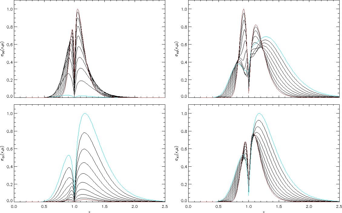
Figure 1: Normalized cross sections for non-resonant, magnetic Compton scattering, integrated over the solid angle $\Omega^{\prime}$ of the outcoming photons, plotted as functions of the ratio $x=\epsilon^{\prime}/\epsilon$ of the ingoing and outgoing photon energies. The curves refer to different values of $\cos\vartheta_{\mathrm{Bk}}$ ranging from 1 (red) to 0.1 (light-blue) with step 0.1 (the integrated cross sections turn out to be symmetric replacing $\theta_{\mathrm{Bk}}$ with $\pi-\theta_{\mathrm{Bk}}$).

Equations (2.1) describe correctly the scattering process in a medium where electrons (and positrons) are substantially at rest in the stellar frame. For the sake of completeness, we discuss here also the general case of electrons and positrons moving at speed $\beta$ (in unit of the speed of light $c$), still treating the scattering in the particle rest frame as conservative. In this case, the expressions for the scattering cross sections in the stellar frame can be obtained from those in the particle rest frame, given by equations (2.1), through the transformation (see Pomraning, 1973)

$$\bar{\sigma}_{ij} =\frac{D}{D^{\prime}}\sigma_{ij}\,,$$ (3)

where

$$D=1-\beta\cos\vartheta_{\mathrm{Bk}}\,\,\,\,\,\,\,\,\,\,\,\,D^{\prime}=1-\beta\cos\vartheta^{\prime}_{\mathrm{Bk}}$$ (4)

and $\vartheta_{\mathrm{Bk}}$ ($\vartheta^{\prime}_{\mathrm{Bk}}$) is the angle between the incoming (outcoming) photon direction and the stellar magnetic field in the star frame. In particular, the angles in the stellar frame can be related to those in the particle frame using the angular aberration formula,

$$\mu_{\mathrm{Bk}}=\frac{\cos\vartheta_{\mathrm{Bk}}-\beta}{D}\,\,\,\,\,\,\,\,\,\,\,\,\mu^{\prime}_{\mathrm{Bk}}=\frac{\cos\vartheta^{\prime}_{\mathrm{Bk}}-\beta}{D^{\prime}}$$ (5)

while, for the energy, it is

$$\varepsilon=\gamma D\epsilon\,\,\,\,\,\,\,\,\,\,\,\,\varepsilon^{\prime}=\gamma D^{\prime}\epsilon^{\prime}\,,$$ (6)

with $\epsilon$ ($\epsilon^{\prime}$) the incoming (outcoming) photon energy in the star reference frame and $\gamma$ the particle Lorentz factor.

Integrating equation (3) in the velocity space of the scattering particles gives the Compton scattering kernel in the stellar frame,

$$\bar{\sigma}_{ij}(\epsilon\rightarrow\epsilon^{\prime},\Omega\rightarrow\Omega^{\prime}) =\int\sigma_{ij}\frac{n_{\mathrm{e}}}{\gamma}\frac{D}{D^{\prime}}f(\beta)\mathrm{d}\beta\,,$$ (7)

in the case of an isotropic velcity distribution. Here $n_{\mathrm{e}}$ is the particle number density and $f(\beta)$ is the particle velocity distribution, which we assume to be a relativistic (1D) maxwellian

$$f(\beta)\mathrm{d}\beta =\frac{\gamma^{3}\mathrm{e}^{-(\gamma-1)/\bar{\Theta}}\mathrm{d}\beta}{2\mathrm{e}^{1/\bar{\Theta}}K_{1}(1/\bar{\Theta})}\,,$$ (8)

with $\bar{\Theta}\equiv kT/m_{\mathrm{e}}c^{2}$ ($T$ is the plasma temperature) and $K_{1}$ the modified Bessel function of the second kind. Finally, using equations (2.1) and (4) – (6), together with the properties of the $\delta$-function, equation (7) becomes

$$\bar{\sigma}_{ij}(\alpha\rightarrow\alpha^{\prime}) =\frac{n_{\mathrm{e}}|\beta|e^{-(\gamma-1)/\bar{\Theta}}}{2\mathrm{e}^{1/\bar{\Theta}}K_{1}(1/\bar{\Theta})}\Sigma_{ij}\,,$$ (9)

where

$$\Sigma_{\mathrm{OO}} \equiv\frac{x(1-\cos^{2}\vartheta_{\mathrm{Bk}})}{\epsilon|x-1|}\frac{(1-\cos^{2}\vartheta^{\prime}_{\mathrm{Bk}})}{\gamma^{3}(1-\beta\cos\vartheta_{\mathrm{Bk}})^{2}(1-\beta\cos\vartheta^{\prime}_{\mathrm{Bk}})^{2}}$$

$$\Sigma_{\mathrm{OX}} \equiv\frac{x(\cos\vartheta_{\mathrm{Bk}}-\beta)^{2}}{\epsilon|x-1|}\left(\frac{\epsilon B_{\mathrm{Q}}}{B}\right)^{2}\gamma^{3}\cos^{2}(\phi_{\mathrm{Bk}}-\phi^{\prime}_{\mathrm{Bk}})$$

$$\Sigma_{\mathrm{XO}} \equiv\frac{x^{3}(\cos\vartheta^{\prime}_{\mathrm{Bk}}-\beta)^{2}}{\epsilon|x-1|}\left(\frac{\epsilon B_{\mathrm{Q}}}{B}\right)^{2}\gamma^{3}\cos^{2}(\phi_{\mathrm{Bk}}-\phi^{\prime}_{\mathrm{Bk}})$$

$$\Sigma_{\mathrm{XX}} \equiv\frac{x(1-\beta\cos\vartheta_{\mathrm{Bk}})^{2}}{\epsilon|x-1|}\left(\frac{\epsilon B_{\mathrm{Q}}}{B}\right)^{2}\gamma^{3}\sin^{2}(\phi_{\mathrm{Bk}}-\phi^{\prime}_{\mathrm{Bk}})$$

and $x\equiv\epsilon^{\prime}/\epsilon$. As an example, Figure 1 shows the behavior of the (normalized) cross sections (9), integrated over the outgoing photon direction, as a function of $x$, for different values of $\cos\vartheta_{\mathrm{Bk}}$ and for $\phi_{\mathrm{Bk}}=0$.

2.2 Radiative transfer in the fireball atmosphere

In this work we treat the fireball plasma as a pure-scattering medium. Since our primary goal in this investigation is to provide and test a general method to compute burst spectral and polarization properties, in the following we restrict to Thomson scattering. The full case of Compton scattering will be addressed in a sequel paper. Among the additional second-order processes that can take place in magnetized plasma, we focus on the effects of double-Compton scattering only, since the contributions of other processes, such as photon splitting and thermal bremsstrahlung, turn out to be far less important under the assumptions we made (see section 5 for a more complete discussion).

Double-Compton scattering is, then, the main process responsible for photon production in the fireball medium. It has been shown (see Lyubarsky, 2002, and references therein) that, at photon energies $\varepsilon\ll\varepsilon_{\mathrm{B}}$, this process can be treated as non-resonant, resembling its non-magnetic counterpart, even when a magnetic field is present. Low-energy photons ($\varepsilon\ll kT$) are injected in the fireball due to double-Compton scattering, at a rate (see Lightman, 1981)

$$Q \approx\frac{4\alpha_{\mathrm{F}}}{3\pi}\frac{\sigma_{\mathrm{T}}}{m_{e}^{2}c^{4}}\frac{\exp(\varepsilon/kT)-1}{\varepsilon^{3}}\left[f_{\mathrm{B}}(\varepsilon,T)-f(\varepsilon)\right]I\,,$$ (11)

where $\alpha_{\mathrm{F}}$ is the fine-structure constant, $f(\varepsilon)$ is the photon occupation number, $f_{\mathrm{B}}(\varepsilon,T)=[\exp(\varepsilon/kT)-1]^{-1}$ and

$$I \equiv\int\varepsilon^{4}[1+f(\varepsilon)]f(\varepsilon)\mathrm{d}\varepsilon\,.$$ (12)

For large scattering depths, equation (11) ensures that photons follow a Planck distribution at photon energies low enough to make double-Compton scattering dominant, $\varepsilon\ll\varepsilon_{0}\approx 0.03(kT)^{3/2}$. At higher energies, on the other hand, scattering tends to establish a Bose-Einstein distribution $f_{\mathrm{BE}}(\varepsilon,T)=[\exp(\varepsilon+\mu/kT)-1]^{-1}$. However, as shown by Lyubarsky (2002), the chemical potential $\mu$ satisfies the condition

$$\ln\frac{\mu+\varepsilon_{0}}{\varepsilon_{0}} \ll 0.5\bigg{(}\frac{10B_{\mathrm{Q}}}{B}\bigg{)}^{2}\,,$$ (13)

where the right-hand side is calculated at scattering depth unity. In this way $\mu$ remains small and one can solve the photon transport assuming local thermal equilibrium (LTE) at large depths for both O- and X-mode photons.

We solved the radiative transfer equations for both the ordinary and the extraordinary photons in the geometrically-thin, surface layers of the fireball which we term the atmosphere. The latter is divided into a number of patches, each labelled by the intensity of the magnetic field at the patch centre and by the angle $\theta_{\mathrm{B}}$ that $\boldsymbol{B}$ makes with the local normal $\boldsymbol{z}$. The contributions from each patch in view are then summed together to derive the overall spectral and polarization properties of the emitted radiation. We assume that the patch dimensions are small enough with respect to the radial scale ($\approx$ the star radius) to neglect the curvature of the closed field lines that contain the fireball. This approach allows us to treat the atmosphere in the plane-parallel approximation, i.e. all the relevant quantities depend only on the height $z$ with respect to the base of the layer. At variance with the case discussed by Lyubarsky (2002), in our model the magnetic field is not necessarily aligned with the patch normal. When this happens, the angle $\theta_{z}$ between the photon direction and $\boldsymbol{z}$ differs from $\theta_{\mathrm{Bk}}$ (see section 2.1), and the two angles are related by

$$\mu_{z} =\mu_{\mathrm{Bk}}\mu_{\mathrm{B}}-\sqrt{(1-\mu^{2}_{\mathrm{Bk}})(1-\mu^{2}_{\mathrm{B}})}\cos\phi_{\mathrm{Bk}}\,,$$ (14)

with $\mu_{z}=\cos\theta_{z}$ and $\mu_{\mathrm{B}}=\cos\theta_{\mathrm{B}}$.

In a pure scattering medium, the radiative transfer equations written in terms of the photon number intensity $n_{i}$ ($i=\mathrm{O,X}$) take the form (see e.g. Mészáros et al., 1989; Alexander et al., 1989),

$$\mu_{z}\frac{\mathrm{d}n_{i}}{\mathrm{d}\tau} =\sum_{k=\mathrm{O,X}}\int\bigg{\{}-\sigma_{ik}(\alpha\rightarrow\alpha^{\prime})n_{i}(\alpha)\big{[}1+n_{k}(\alpha^{\prime})\big{]}$$

$$\,\,\,\,\,\,+\sigma_{ki}(\alpha^{\prime}\rightarrow\alpha)\bigg{(}\frac{\varepsilon^{\prime}}{\varepsilon}\bigg{)}^{2}n_{k}(\alpha^{\prime})\big{[}1+n_{i}(\alpha)\big{]}\bigg{\}}\mathrm{d}\varepsilon^{\prime}\mathrm{d}\Omega^{\prime}\,,$$ (15)

where stimulated scattering is accounted for. Here $\mathrm{d}\tau=n_{\mathrm{e}}\sigma_{\mathrm{T}}\mathrm{d}s$ is the infinitesimal Thomson depth, with $s$ a parameter along the photon propagation direction. However the previous expression can be considerably simplified. In fact, in LTE the scattering cross sections (2.1) must obey the detailed balance condition (see e.g. Mészáros et al., 1989; Alexander et al., 1989; Alexander & Mészáros, 1991),

$$\sigma_{ki}(\alpha^{\prime}\rightarrow\alpha) =\bigg{(}\frac{\varepsilon}{\varepsilon^{\prime}}\bigg{)}^{2}\exp\big{[}-(\varepsilon-\varepsilon^{\prime})/kT\big{]}\sigma_{ik}(\alpha\rightarrow\alpha^{\prime})\,;$$ (16)

in this way, equation (2.2) becomes

$$\mu_{z}\frac{\mathrm{d}n_{i}}{\mathrm{d}\tau} =\sum_{k=\mathrm{O,X}}\int\bigg{\{}-\sigma_{ik}(\alpha\rightarrow\alpha^{\prime})n_{i}(\alpha)$$

$$\,\,\,\,\,\,+\sigma_{ik}(\alpha\rightarrow\alpha^{\prime})F_{i}(\alpha,\varepsilon^{\prime})n_{k}(\alpha^{\prime})\bigg{\}}\mathrm{d}\varepsilon^{\prime}\mathrm{d}\Omega^{\prime}\,,$$ (17)

where

$$F_{i}(\alpha,\varepsilon^{\prime}) \equiv\exp\big{[}-(\varepsilon-\varepsilon^{\prime})/kT\big{]}\bigg{(}1+n_{i}(\alpha)\bigg{)}-n_{i}(\alpha)\,.$$ (18)

Finally, under the assumption of conservative scattering ($\varepsilon=\varepsilon^{\prime}$) and substituting the expressions (2.1), one obtains

$$\mu_{z}\frac{\mathrm{d}n_{\mathrm{O}}}{\mathrm{d}\tau} =-\bigg{[}1-\mu^{2}_{\mathrm{Bk}}+\frac{3\mu^{2}_{\mathrm{Bk}}}{4}\bigg{(}\frac{\varepsilon}{\varepsilon_{\mathrm{B}}}\bigg{)}^{2}\bigg{]}n_{\mathrm{O}}(\alpha)$$

$$\,\,\,\,\,\,+\frac{3}{8\pi}\int_{4\pi}\bigg{[}(1-\mu_{\mathrm{Bk}}^{2})(1-\mu_{\mathrm{Bk}}^{\prime 2})n_{\mathrm{O}}(\alpha^{\prime})$$

$$\,\,\,\,\,\,+\bigg{(}\frac{\varepsilon}{\varepsilon_{\mathrm{B}}}\bigg{)}^{2}\mu^{2}_{\mathrm{Bk}}\cos^{2}(\phi_{\mathrm{Bk}}-\phi^{\prime}_{\mathrm{Bk}})n_{\mathrm{X}}(\alpha^{\prime})\bigg{]}\mathrm{d}\Omega^{\prime}$$

$$\mu_{z}\frac{\mathrm{d}n_{\mathrm{X}}}{\mathrm{d}\tau} =-\bigg{(}\frac{\varepsilon}{\varepsilon_{\mathrm{B}}}\bigg{)}^{2}n_{\mathrm{X}}(\alpha)$$

$$\,\,\,\,\,\,+\frac{3}{8\pi}\bigg{(}\frac{\varepsilon}{\varepsilon_{\mathrm{B}}}\bigg{)}^{2}\int_{4\pi}\bigg{[}\sin^{2}(\phi_{\mathrm{Bk}}-\phi^{\prime}_{\mathrm{Bk}})n_{\mathrm{X}}(\alpha^{\prime})$$

$$\,\,\,\,\,\,+\mu^{\prime 2}_{\mathrm{Bk}}\cos^{2}(\phi_{\mathrm{Bk}}-\phi^{\prime}_{\mathrm{Bk}})n_{\mathrm{O}}(\alpha^{\prime})\bigg{]}\mathrm{d}\Omega^{\prime}\,.$$ (19)

As discussed in the previous section, the propagation of photons in the fireball medium is quite different according to their polarization mode. These two different behaviors can be described in terms of the O- and X-mode optical depths $\tau_{i}\sim n_{\mathrm{e}}\sigma_{i}H$ ($i=\mathrm{O,\,X}$), where $\sigma_{i}=\int(\sigma_{i\mathrm{O}}+\sigma_{i\mathrm{X}})\mathrm{d}\varepsilon^{\prime}\mathrm{d}\Omega^{\prime}$ and $H$ is the scale height of the fireball atmospheric layer. Taking into account the cross sections (2.1) it results

$$\tau_{\mathrm{O}} \approx\tau$$

$$\tau_{\mathrm{X}} =\left(\frac{\varepsilon}{\varepsilon_{\mathrm{B}}}\right)^{2}\tau_{\mathrm{O}}\,,$$ (20)

with $\tau$ the Thomson scattering depth. We remind that these considerations and the following equations hold in the limit $\varepsilon\ll\varepsilon_{\mathrm{B}}$. Owing to the suppression factor $(\varepsilon/\varepsilon_{\mathrm{B}})^{2}$ of the X-mode photon cross section with respect to the O-mode one (see section 2.1), the photosphere of X-mode photons (i.e. the layer at which $\tau_{\mathrm{X}}\approx 1$) lies at different heights in the fireball atmosphere for photons with different energies; in particular, it is closer to the top the higher the photon energy. At the same time, it is $\tau_{\mathrm{O}}\gg 1$ at the X-mode photosphere for all the energies of interest ($\sim$ 1–100 keV).

For these reasons, we follow the approach described by Lyubarsky (2002) and solve the photon transport in terms of the Rosseland mean optical depth $\tau_{\mathrm{R}}$ for the X-mode photons, defined by

$$\mathrm{d}\tau_{\mathrm{R}} =n_{\mathrm{e}}\sigma_{\mathrm{X,R}}\mathrm{d}s\,,$$ (21)

where $\sigma_{\mathrm{X,R}}$ is the Rosseland mean of the $\sigma_{\mathrm{X}}$ cross section

$$\sigma_{\mathrm{X,R}} =\left[\frac{\int\sigma_{\mathrm{X}}^{-1}\partial B_{\varepsilon}/\partial T\,\mathrm{d}\varepsilon}{\int\partial B_{\varepsilon}/\partial T\,\mathrm{d}\varepsilon}\right]^{-1}$$

$$=\frac{4\pi^{2}}{5}\sigma_{\mathrm{T}}\left(\frac{kTB_{\mathrm{Q}}}{m_{\mathrm{e}}c^{2}B}\right)^{2}\,,$$ (22)

with $B_{\varepsilon}(T)=\varepsilon^{3}/[\exp(\varepsilon/kT)-1]$. A good approximation for the temperature distribution can be obtained, in the diffusion regime ($\tau>1$), for a scattering dominated medium (see Lyubarsky, 2002, and references therein),

$$T =T_{\mathrm{b}}\sqrt{1+\frac{3}{4}\tau_{\mathrm{R}}}\,.$$ (23)

where $T_{\mathrm{b}}$ is the bolometric temperature. Actually, solving the temperature profile in this particular case is a non-trivial problem, since it involves the computation of the energy exchange between the radiation field and the pair plasma in the presence of double-Compton and non-conservative scattering. Strictly speaking, the validity of equation (23) is restricted to the optically thick limit. However, it provides a good approximation to the numerical solution one obtains solving the energy balance in the fireball medium also at small optical depths, as we checked a posteriori. Deviations turn out to be $\la 15\%$, in agreement with what found also by Lyubarsky (2002). The Rosseland mean optical depth follows from equations (2.2) and (23),

$$\tau_{\mathrm{R}} =\frac{4\pi^{2}}{5}\left(\frac{kT_{\mathrm{b}}B_{\mathrm{Q}}}{m_{\mathrm{e}}c^{2}B}\right)^{2}\sigma_{\mathrm{T}}\int n_{\mathrm{e}}\mathrm{d}s=R(B)\tau\,,$$ (24)

where

$$R(B) \equiv\frac{4\pi^{2}}{5}\left(\frac{kT_{\mathrm{b}}B_{\mathrm{Q}}}{m_{\mathrm{e}}c^{2}B}\right)^{2}\,.$$ (25)

This allows to relate the optical depths $\tau_{\mathrm{O}}$ and $\tau_{\mathrm{X}}$

$$\tau_{\mathrm{O}} =\frac{5}{4\pi^{2}}\left(\frac{m_{\mathrm{e}}c^{2}B}{kT_{\mathrm{b}}B_{\mathrm{Q}}}\right)^{2}\tau_{\mathrm{R}}\,,\,\,\,\,\,\,\,\,\,\,\,\,\,\,\,\tau_{\mathrm{X}}=\frac{5}{4\pi^{2}}\left(\frac{\varepsilon}{kT_{\mathrm{b}}}\right)^{2}\tau_{\mathrm{R}}\,.$$ (26)

Finally, using equation (24) one can rewrite the radiative transfer equations (2.2) in terms of the Rosseland mean optical depth simply scaling the right-hand sides of both of them by the factor $R(B)$:

$$\mu_{z}\frac{\mathrm{d}n_{\mathrm{O}}}{\mathrm{d}\tau_{\mathrm{R}}} =-\frac{1}{R(B)}\bigg{\{}\bigg{[}1-\mu^{2}_{\mathrm{Bk}}+\frac{3\mu^{2}_{\mathrm{Bk}}}{4}\bigg{(}\frac{\varepsilon}{\varepsilon_{\mathrm{B}}}\bigg{)}^{2}\bigg{]}n_{\mathrm{O}}(\alpha)$$

$$\,\,\,\,\,\,+\frac{3}{8\pi}\int_{4\pi}\bigg{[}(1-\mu_{\mathrm{Bk}}^{2})(1-\mu_{\mathrm{Bk}}^{\prime 2})n_{\mathrm{O}}(\alpha^{\prime})$$

$$\,\,\,\,\,\,+\bigg{(}\frac{\varepsilon}{\varepsilon_{\mathrm{B}}}\bigg{)}^{2}\mu^{2}_{\mathrm{Bk}}\cos^{2}(\phi_{\mathrm{Bk}}-\phi^{\prime}_{\mathrm{Bk}})n_{\mathrm{X}}(\alpha^{\prime})\bigg{]}\mathrm{d}\Omega^{\prime}\bigg{\}}$$

$$\mu_{z}\frac{\mathrm{d}n_{\mathrm{X}}}{\mathrm{d}\tau_{\mathrm{R}}} =-\frac{1}{R(B)}\bigg{\{}\bigg{(}\frac{\varepsilon}{\varepsilon_{\mathrm{B}}}\bigg{)}^{2}n_{\mathrm{X}}(\alpha)$$

$$\,\,\,\,\,\,+\frac{3}{8\pi}\bigg{(}\frac{\varepsilon}{\varepsilon_{\mathrm{B}}}\bigg{)}^{2}\int_{4\pi}\bigg{[}\sin^{2}(\phi_{\mathrm{Bk}}-\phi^{\prime}_{\mathrm{Bk}})n_{\mathrm{X}}(\alpha^{\prime})$$

$$\,\,\,\,\,\,+\mu^{\prime 2}_{\mathrm{Bk}}\cos^{2}(\phi_{\mathrm{Bk}}-\phi^{\prime}_{\mathrm{Bk}})n_{\mathrm{O}}(\alpha^{\prime})\bigg{]}\mathrm{d}\Omega^{\prime}\bigg{\}}\,.$$ (27)

3 Numerical implementation

In this section we illustrate the numerical method we used to compute the spectra of the photons emitted from a typical magnetar fireball. Hereafter we will refer to a template neutron star with radius $R_{\mathrm{NS}}=10$ km and mass $M_{\mathrm{NS}}=1.4\,M_{\mathrm{\odot}}$.

3.1 Integration of the radiative transfer equations

We developed a specific fortran code to solve the radiative transfer in the fireball atmosphere described in section 2.2. We assumed a maximum optical depth $\tau_{\mathrm{R}}^{\mathrm{max}}=1000$ at the base of the fireball atmosphere, since this guarantees that the medium is optically thick for X-mode photons over the entire energy range $1$–$100$ keV. The optical depth varies between $\tau_{\mathrm{R}}^{\mathrm{max}}$ at the base and $\tau_{\mathrm{R}}^{\mathrm{min}}=0$ at the top and is sampled by a non-uniform, 500-point grid. However, such a high value for $\tau_{\mathrm{R}}^{\mathrm{max}}$ implies extremely large values of $\tau_{\mathrm{O}}$ (at the strongest magnetic fields) and $\tau_{\mathrm{X}}$ (at high energies), which make the computational time totally unacceptable. For this reason we decide to integrate the two radiative transfer equations (2.2) for $\tau_{\mathrm{O},\mathrm{X}}\leq 10$ only, taking $n_{\mathrm{O},\mathrm{X}}$ as Planck distributions at the local temperature $T$ otherwise. Since, for the chosen values of the parameters, the X-mode photosphere lies always at larger $\tau_{\mathrm{R}}$ with respect to the O-mode one, we partially modify the second of the equations (2.2) in the case of $\tau_{\mathrm{X}}\leq 10$ and $\tau_{\mathrm{O}}>10$ taking the number intensity $n_{\mathrm{O}}$ that appears at the right-hand side as planckian (see also Lyubarsky, 2002).

As discussed in section 2.2, the fireball atmosphere is divided into 30 plane-parallel slabs, labelled by the values of $B$ at their centres. The (dipolar) magnetic field at the pole is taken to be $2\times 10^{14}$ G, which results in a minimum value of $B\sim 10^{13}$ G at the magnetic equator for $R_{\mathrm{max}}=2R_{NS}$, i.e. at the largest radial distance reached by the fireball. The angle $\theta_{\mathrm{B}}$ between the stellar $B$-field and the local normal is always $90^{\circ}$, because, along the field lines, the magnetic field $\boldsymbol{B}$ at the patch centre is always perpendicular to the local normal. For the sake of simplicity, we assume $\boldsymbol{B}$ as constant over each patch, i.e. we neglect its variation in both direction and intensity within the slab. It can be verified that the error amounts at most to $\Delta B/B\sim 3\%$. For each patch the temperature distribution (23) has been assumed, with a bolometric temperature $T_{\mathrm{b}}=10$ keV.

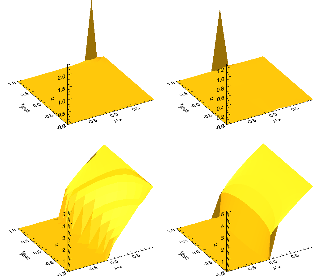
Figure 2: Number intensities $n_{\mathrm{O}}$ (top row) and $n_{\mathrm{X}}$ (bottom row) of the emerging radiation, plotted as functions of $\mu_{z}$ and $\cos\phi_{z}$ in the cases of two patches characterized by $\theta_{\mathrm{B}}=45^{\circ}$ (left-hand column) and $\theta_{\mathrm{B}}=90^{\circ}$ (right-hand column); the magnetic field intensity is $B=10^{14}$ G.

In order to solve the radiative transfer equations in each slab, the code uses a simple $\Lambda$-iteration. In fact, both the equations (2.2) can be written in the compact form

$$\frac{\mathrm{d}n_{i}}{\mathrm{d}\tau_{\mathrm{R}}} =C_{i}n_{i}-S_{i}\,\,\,\,\,\,\,\,\,(i=\mathrm{O},\,\mathrm{X})\,,$$ (28)

where $C_{i}$ does not depend on $\tau_{\mathrm{R}}$ and $S_{i}$ represents the source term, that contains the integrals of $n_{i}$ over the angles $\theta^{\prime}_{\mathrm{Bk}}$ and $\phi^{\prime}_{\mathrm{Bk}}$. The Sommerfeld radiative condition is imposed at the top of the slab, i.e. $n_{i}=0$ for $-1\leq\mu_{z}\leq 0$ at $\tau_{\mathrm{R}}=0$. Integration is started making an initial guess for $n_{i}$ and the initial source terms $S^{(0)}_{i}$ are then calculated through a Gauss-Lobatto quadrature, using a 20-point grid for both $\mu^{\prime}_{\mathrm{Bk}}$ and $\phi^{\prime}_{\mathrm{Bk}}$. With these values for the source terms, the code integrates the radiative transfer equations using a Runge-Kutta, fourth order method, following a set of rays sampled by a 20$\times$20 mesh in $-1\leq\mu_{\mathrm{Bk}}\leq 1$ and $0\leq\phi_{\mathrm{Bk}}\leq 2\pi$. The new values of $n_{i}$ are used to calculate the source terms $S^{(1)}_{i}$ at the next step. The iterative method proceeds until the fractional accuracy

$$\Delta =\frac{|S_{i}^{(n)}-S_{i}^{(n-1)}|}{|S_{i}^{(n)}|+|S_{i}^{(n-1)}|}$$ (29)

drops below a given value. The same procedure is repeated for different values of the photon energy $\varepsilon$, ranging between 1 and 100 keV within an equally-spaced, 30-point grid.

The code returns the number intensity $n_{i}$ as a function of the optical depth $\tau$ in the slab, the photon energy $\varepsilon$ and the angles $\theta_{\mathrm{Bk}}$ and $\phi_{\mathrm{Bk}}$ that the photon direction makes with the stellar magnetic field at the patch centre. This has been done for 30 selected values of the magnetic field intensity (equally spaced in log between $10^{13}$ and $2\times 10^{14}$ G). Figure 2 presents the angular distribution of the emerging radiation ($\tau_{\mathrm{R}}=0$) for both ordinary and extraordinary photons; for comparison, two different values of $\theta_{\mathrm{B}}=45^{\circ}$ and $90^{\circ}$ are shown. In all the panels, the intensities are plotted as functions of $\mu_{z}$ and $\cos\phi_{z}$, where the latter is the azimuthal angle associated to $\theta_{z}$ (see section 2.2). Ordinary photons appear to be beamed along the local magnetic field direction, at variance with the extraordinary ones. Figure 3 shows instead the behavior of the total, O-mode and X-mode photon number fluxes as functions of the energy for two different patches, with $\theta_{\mathrm{B}}=90^{\circ}$ and $B=10^{13}$, $10^{14}$ G, respectively. In both the panels it can be clearly seen the flattening of the emerging spectrum at low energies, due to the fact that X-mode photons with lower energies escape the fireball medium from regions with higher temperature (see Lyubarsky, 2002). Moreover, the extraordinary photon flux turns out to be well above the ordinary one especially for low energies, as expected since the O-mode optical depth is much larger than the X-mode one (see section 2.2). This difference is enhanced for increasing magnetic field intensities, when the X-mode flux dominates over the O-mode one in the entire energy range.

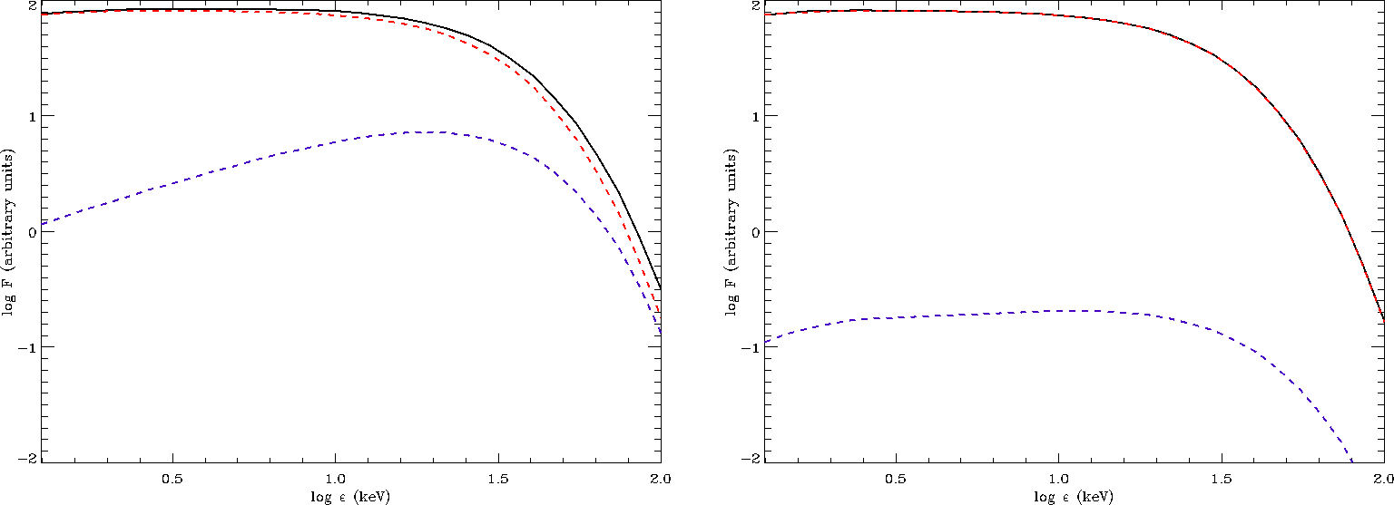
Figure 3: Photon number fluxes in the case of two single patches characterized by $\theta_{\mathrm{B}}=90^{\circ}$, $B=10^{13}$ (left panel) and $10^{14}$ G (right panel), plotted as functions of the photon energy. The black, solid line represents the total spectrum, while the blue and red dashed lines the O-mode and X-mode photon spectra, respectively.

3.2 Ray-tracing

The data generated by the radiative transfer code described above are then processed in an idl ray-tracer code, in order to simulate the spectra of the emitted radiation and the polarization observables at infinity as functions of photon energy and rotational phase. The code is discussed in detail in Taverna et al. (2015, see also ); given that the geometry (see below) is more complicated in the present case, no GR corrections are included.

3.2.1 Geometry

The neutron star geometry is described in a fixed frame $(X,Y,Z)$ where the $Z$ axis is chosen along the line-of-sight (LOS, unit vector $\boldsymbol{\ell}$) and the $X$ axis is in the plane made by $\boldsymbol{\ell}$ and the star spin axis $\boldsymbol{\Omega}$. However it is convenient to introduce also a reference frame $(p,q,t)$ which rotates around $\boldsymbol{\Omega}$, with the $t$ axis along the star magnetic axis (unit vector $\boldsymbol{b}_{\mathrm{dip}}$). Denoting with $\chi$ and $\xi$ the angles that the rotation axis makes with $\boldsymbol{\ell}$ and $\boldsymbol{b}_{\mathrm{dip}}$, respectively, the unit vectors that define the $\boldsymbol{b}_{\mathrm{dip}}$ reference frame can be expressed in the LOS frame as (see e.g. Taverna et al., 2015)

$$\boldsymbol{p} =(-\sin\chi\sin\xi-\cos\chi\cos\xi\cos\gamma,\cos\xi\sin\gamma,$$

$$\,\,\,\,\,\,\,\,\,\sin\chi\cos\xi\cos\gamma-\cos\chi\sin\xi)$$

$$\boldsymbol{q} =(-\cos\chi\sin\gamma,-\cos\gamma,\sin\chi\sin\gamma)$$

$$\boldsymbol{t} \equiv\boldsymbol{b}_{\mathrm{dip}}=(\sin\chi\cos\xi-\cos\chi\sin\xi\cos\gamma,\sin\xi\sin\gamma,$$

$$\,\,\,\,\,\,\,\,\,\,\,\,\,\,\,\,\,\,\,\,\,\,\,\,\,\,\,\cos\eta)\,,$$ (30)

where $\gamma$ is the star rotational phase and $\cos\eta=\cos\chi\cos\xi+\sin\chi\sin\xi\cos\gamma$ is the cosine of the angle between $\boldsymbol{\ell}$ and $\boldsymbol{b}_{\mathrm{dip}}$.

The position of a generic point on the surface of the fireball is given by $\boldsymbol{r}=r(\sin\Theta\cos\Phi,\sin\Theta\sin\Phi,\cos\Theta)$ in the LOS reference frame, where the radial distance $r$ is given by the relation

$$r =R_{\mathrm{max}}\sin^{2}\theta\,.$$ (31)

Because $r\geq R_{\mathrm{NS}}$, the magnetic colatitude $\theta$ is in the range $[\theta_{\mathrm{min}},\theta_{\mathrm{max}}]$, with

$$\theta_{\mathrm{min}} =\arcsin\left(\sqrt{\frac{R_{\mathrm{NS}}}{R_{\mathrm{max}}}}\right)$$ (32)

and $\theta_{\mathrm{max}}=\pi-\theta_{\mathrm{min}}$. This holds for each value of the magnetic azimuth $\phi$, that ranges between $0$ and $2\pi$ if the fireball is assumed to be torus-like, i.e. it fills the entire volume between the star surface and the limiting field lines given by equation (31); for the sake of conciseness, in the following we will refer to this volume as the fireball torus. The polar angles $\theta$ and $\phi$ in the $\boldsymbol{b}_{\mathrm{dip}}$ frame are then related to $\Theta$ and $\Phi$ in the LOS frame by

$$\cos\theta =\boldsymbol{r}\cdot\boldsymbol{b}_{\mathrm{dip}}$$

$$\cos\phi =\boldsymbol{r}_{\perp}\cdot\boldsymbol{p}\,,$$ (33)

where

$$\boldsymbol{r}_{\perp} =\frac{\boldsymbol{r}-(\boldsymbol{b}_{\mathrm{dip}}\cdot\boldsymbol{r})\boldsymbol{b}_{\mathrm{dip}}}{|\boldsymbol{r}-(\boldsymbol{b}_{\mathrm{dip}}\cdot\boldsymbol{r})\boldsymbol{b}_{\mathrm{dip}}|}$$ (34)

is the (normalized) projection of the position vector $\boldsymbol{r}$ in the plane perpendicular to $\boldsymbol{b}_{\mathrm{dip}}$.

We consider also the case in which the azimuthal extension of the fireball is restricted between two given values $\phi_{\mathrm{min}}$ and $\phi_{\mathrm{max}}$, so that the emitting surface consists of a portion of the torus plus the two constant-$\phi$ cuts. Of course, the magnetic field is perpendicular to the surface normal also within the two $\phi_{\mathrm{min}},\phi_{\mathrm{max}}$ “sides” of the torus. For shortness, we will refer hereafter to the case of emission from the entire torus as “model a”, while we will call “model b” that in which emission is limited to the portion of the fireball between $\phi_{\mathrm{min}}$ and $\phi_{\mathrm{max}}$ (with the emission from the two sides included).

3.2.2 Fireball visibility

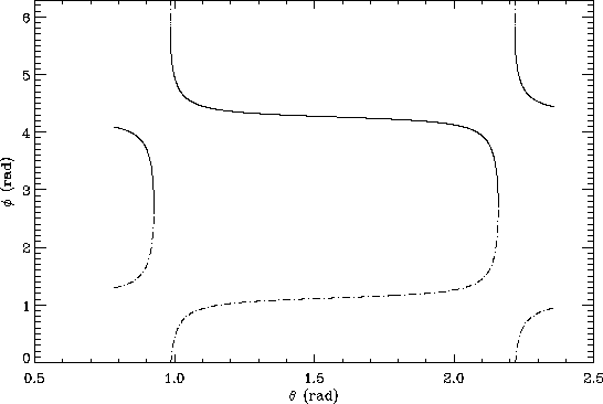
Figure 4: Behavior of the first (solid line) and of the second (dash-dotted line) solutions of equation (41), plotted as functions of the magnetic colatitude $\theta$, for $\chi=60^{\circ}$, $\xi=30^{\circ}$ and $\gamma=150^{\circ}$. Notice that the dash-dotted solution has been reduced to the $[0,2\pi]$ range.

Figure 5: Limiting field lines (yellow lines) of a torus-shaped fireball for $\chi=60^{\circ}$, $\xi=30^{\circ}$ and $\gamma=150^{\circ}$, seen both along the LOS ($Z$ axis, left-hand panel) and slightly rotated around the $Y$ axis (right-hand panel); the field lines corresponding to $\phi=0^{\circ},\,90^{\circ},\,180^{\circ},\,270^{\circ}$ are highlighted in black, violet, green and dark blue, respectively. The terminator is marked by the light blue line, while the region in view of the fireball surface is marked by the red lines.

To determine the portion of the fireball surface which is in view once the values of the geometrical angles $\chi$ and $\xi$ have been fixed, the code calculates the terminator of the surface, that is given by the condition

$$\boldsymbol{z}\cdot\boldsymbol{\ell} =0\,,$$ (35)

where $\boldsymbol{z}$ denotes the local surface normal unit vector. The calculation turns out to be simpler in the $\boldsymbol{b}_{\mathrm{dip}}$ reference frame; here the LOS unit vector $\boldsymbol{\ell}$ takes the form $\boldsymbol{\ell}=(\sin\eta\cos\delta,\sin\eta\sin\delta,\cos\eta)$, with $\delta$ the azimuth of the LOS with respect to $\boldsymbol{b}_{\mathrm{dip}}$, while the components of the local normal $\boldsymbol{z}$ are derived in Appendix A. In particular, $\delta$ is related to the angles $\chi$, $\xi$ and $\gamma$ through the scalar product

$$\cos\delta =\boldsymbol{p}\cdot\boldsymbol{\ell}_{\perp}\,,$$ (36)

that can be calculated in the LOS frame, where the components of the unit vector $\boldsymbol{p}$ are given by the first of equations (3.2.1), while those of the normalized projection $\boldsymbol{\ell}_{\perp}$ of the LOS orthogonal to $\boldsymbol{b}_{\mathrm{dip}}$ result

$$\boldsymbol{\ell}_{\perp} =\frac{1}{\sin\eta}\left(\begin{array}[]{c}-b_{\mathrm{dip,X}}\cos\eta\\ -b_{\mathrm{dip,Y}}\cos\eta\\ 1-b_{\mathrm{dip,Z}}\cos\eta\end{array}\right)\,.$$ (40)

Using equation (73), the condition (35) translates into the following equation,

$$\cos(\phi-\delta) =\frac{3\sin\theta\cos\theta\cos\eta}{\sin\eta(3\cos^{2}\theta-1)}\,,$$ (41)

which can be solved only if the condition

$$\left|\frac{3\sin\theta\cos\theta\cos\eta}{\sin\eta(3\cos^{2}\theta-1)}\right| <1$$ (42)

is satisfied (the details of the calculations are discussed in Appendix B). The solutions of equation (41) can be written in the simple form

$$\phi=\arccos A+\delta\,\,\,\cup\,\,\,\phi=(2\pi-\arccos A)+\delta\,,$$ (43)

where $A$ denotes the right-hand side of equation (41) for $\theta$ belonging to the domain (B). Since both $A$ and $\delta$ depend on the values of $\chi$, $\xi$ and the rotational phase $\gamma$, the shape of the surface terminator will change for different viewing geometries. As an example, Figure 4 shows the behavior of the two solutions (43) for $\chi=60^{\circ}$, $\xi=30^{\circ}$ and $\gamma=150^{\circ}$. It can be clearly seen that, for the given values of the viewing angles, the solutions exist only within the three intervals $I_{1}=[\theta_{\mathrm{min}},a_{1}]$, $I_{2}=[a_{4},b_{1}]$ and $I_{3}=[b_{4},\theta_{\mathrm{max}}]$, where $a_{1}$, $a_{4}$, $b_{1}$ and $b_{4}$ are defined in equation (B). Figure 5 shows the terminator and the part in view of the fireball surface for the same values of $\chi$, $\xi$ and $\gamma$.

Having calculated the polar angles $\theta$ and $\phi$ that characterize the terminator in the $\boldsymbol{b}_{\mathrm{dip}}$ reference frame, it remains to determine which points on the fireball surface are in view. The code first calculates the values of colatitude $\theta_{\mathrm{term}}^{\pm}$ that identify the terminator at each given value of the magnetic azimuth $\phi$. This is equivalent to draw a horizontal line in the plot of Figure 4, and find the intersections of this line with the curves. The latter can be found inverting equation (41),

$$\tan\theta_{\mathrm{term}}^{\pm} =\frac{-3\cos\eta\pm\sqrt{9\cos^{2}\eta+8\cos^{2}\big{(}\phi-\delta\big{)}\sin^{2}\eta}}{2\cos\big{(}\phi-\delta\big{)}\sin\eta}\,.$$ (44)

Figure 6: Phase-averaged total (black, solid line), ordinary (blue, dashed line) and extraordinary (red, dashed line) photon spectra obtained from the ray-tracer code in the case of model a, for $\chi=60^{\circ}$ and $\xi=30^{\circ}$ (i.e. the case shown in Figure 5).

Taking e.g. $\phi=\pi$, equation (44) gives two values $\theta_{\mathrm{term}}^{\pm}$ that correspond to the terminator and lie in the intervals $I_{1}$ and $I_{2}$ defined above. These two terminator points are clearly visible in Figure 5, where the field line corresponding to $\phi=\pi$ is marked in green; specifically, it can be seen that the only points along the field line that are in view are those included between the two values $\theta_{\mathrm{term}}^{\pm}$. On the other hand, in the case $\phi=3\pi/2$ Figure 4 shows that the two solutions $\theta_{\mathrm{term}}^{\pm}$ of equation (44) belong to the intervals $I_{2}$ and $I_{3}$. In this case, the points in view along the field line (see the dark-blue line in Figure 5b) are those connecting $\theta_{\mathrm{min}}$ and the smaller of $\theta_{\mathrm{term}}^{\pm}$. Although this qualitative reasoning has been discussed for two values of $\phi$ only, it allows to get a general rule that holds for whatever field line, labeled by a generic magnetic azimuth. Given a value of $\phi$, the points of the field line in view are those with $\theta$ between the two solutions $\theta_{\mathrm{term}}^{\pm}$ (given in equation 44) if one of them belong to the interval $I_{1}$; only the points with colatitude within $\theta_{\mathrm{min}}$ and the smaller of $\theta_{\mathrm{term}}^{\pm}$ will be in view otherwise.

In the case in which the fireball is limited azimuthally between $\phi_{\mathrm{min}}$ and $\phi_{\mathrm{max}}$, a different visibility condition has to be imposed for the two constant-$\phi$ “sides”. Actually, since we assumed that these two surfaces are planar, the problem can be simply solved checking the sign of $\boldsymbol{\ell}\cdot\boldsymbol{h}$, with $\boldsymbol{h}$ the outgoing normal to the constant-$\phi$ slice. If this scalar product is positive then all the points of the slice are in view. In particular, in the $\boldsymbol{b}_{\mathrm{dip}}$ reference frame, the unit vector $\boldsymbol{h}$ for each of the two slices can be expressed as

$$\boldsymbol{h} =\pm\,\boldsymbol{m}\times\boldsymbol{b}_{\mathrm{dip}}\,,$$ (45)

where the $+$ ($-$) sign corresponds to $\bar{\phi}=\phi_{\mathrm{min}}$ ($\phi_{\mathrm{max}}$) and $\boldsymbol{m}$ is the (unit) position vector of the generic point in the plane $\phi=\bar{\phi}$ (see the first equality in equation 67). By choosing, for the sake of simplicity, $\theta=\pi/2$, one readily obtains

$$\boldsymbol{h}=\left(\begin{array}[]{c}\pm\sin\bar{\phi}\\ \mp\cos\bar{\phi}\\ 0\end{array}\right)\,.$$ (49)

By deriving the components $(h_{X},h_{Y},h_{Z})$ in the LOS frame (see Appendix C), the visibility condition can be then written as $h_{Z}>0$.

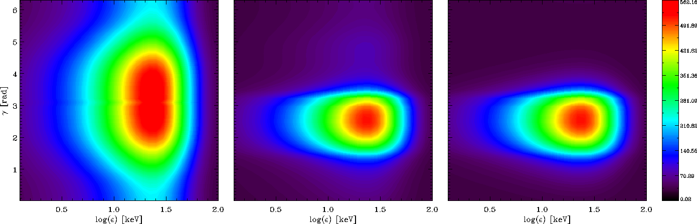
Figure 7: Total intensity (arbitrary units), plotted as a function of the photon energy $\varepsilon$ and the rotational phase $\gamma$, in the case of model a (left-hand panel) and model b with $\phi_{\mathrm{min}}=100^{\circ}$ and $\phi_{\mathrm{max}}=190^{\circ}$ (central panel). The right-hand panel shows the same case as the central one, but without including emission from the planar slices at the sides. As in Figure 6, it is $\chi=60^{\circ}$ and $\xi=30^{\circ}$.

Finally, one needs to exclude, from the part in view of both the torus and the slices found with the methods discussed above, the region covered by the star projection in the plane of the sky. This can be easily performed transforming the coordinates of the position vector $\boldsymbol{m}$ of each point in view from the $\boldsymbol{b}_{\mathrm{dip}}$ frame (see equation 67) to the LOS one. Hence, the points covered by the star are identified by the condition

$$m^{2}_{X}+m^{2}_{Y}<1\,\,\,\cap\,\,\,m_{Z}<1$$ (50)

and can be excluded. The result of this operation is evident in Figure 5b.

3.2.3 Photon flux and polarization observables

In the ray-tracer code the entire fireball surface is divided into a $100$$\times$$100$ angular mesh in $(\Theta,\Phi)$, where $0<\Theta<\pi$ and $0<\Phi<2\pi$, while each of the two sides at $\phi_{\mathrm{min}}$ and $\phi_{\mathrm{max}}$ (if present) is divided through a $(r,\theta)$ grid with $\theta_{\mathrm{min}}\leq\theta\leq\theta_{\mathrm{max}}$ and $R_{\mathrm{NS}}\leq r\leq R_{\mathrm{max}}\sin^{2}\theta$ (in the actual calculation a $50\times 10$ mesh was used). Once the visible part of the fireball is known, any given patch is characterized by the value of the strength $B$ of the magnetic field and by the polar angles $\theta_{\mathrm{Bk}}$ and $\phi_{\mathrm{Bk}}$ that the ray which reaches the observer (i.e. which propagates along the LOS) makes with the local $B$-field direction. Then, the code calculates the total photon flux and the polarization observables summing the contributions from the single surface patches. In this respect, it is important to notice that the surface element takes different forms according to which part of the fireball (the toroidal surface or the “sides”) is considered. In particular, for the toroidal surface, one has in the LOS reference frame

$$\mathrm{d}A_{1} =r^{2}\sin\Theta\mathrm{d}\Theta\mathrm{d}\Phi=R^{2}_{\mathrm{max}}\sin^{4}\theta\sin\Theta\mathrm{d}\Theta\mathrm{d}\Phi\,,$$ (51)

where equation (31) has been used and $\sin^{4}\theta$ can be written as a function of $\Theta$ and $\Phi$ using the first of equations (3.2.1). Instead, for the two azimuthal slices, it is convenient to express the surface element in the $\boldsymbol{b}_{\mathrm{dip}}$ frame, obtaining

$$\mathrm{d}A_{2} =r\mathrm{d}r\mathrm{d}\theta\,.$$ (52)

Therefore, the total photon flux $F_{\mathrm{I}}$ will be the sum of the two contributions $F_{I,1}$ and $F_{I,2}$, with

$$F_{\mathrm{I},j} =F_{\mathrm{O},j}+F_{\mathrm{X},j}=\int\big{(}n_{\mathrm{O}}+n_{\mathrm{X}}\big{)}P_{j}\mathrm{d}A_{j}\,;$$ (53)

here the symbol $P_{j}$ represents the projection factor,

$$P_{1} =\boldsymbol{z}\cdot\boldsymbol{\ell}\ \ \ \ \ \ \ \ \ \ P_{2}=\boldsymbol{h}\cdot\boldsymbol{\ell}\,,$$ (54)

where $\boldsymbol{z}$ and $\boldsymbol{h}$ are defined by equations (73) and (49), respectively.

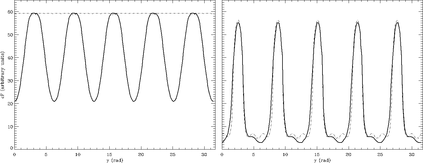
Figure 8: Pulse profile of the radiation emitted from the fireball in the case of model a (left-hand panel) and model b (with $\phi_{\mathrm{min}}=100^{\circ}$ and $\phi_{\mathrm{max}}=190^{\circ}$, right-hand panel), calculated in the $10$–$50$ keV energy range. Here the solid lines refers to the case $\chi=60^{\circ}$, $\xi=30^{\circ}$ and the dash-dotted lines to the case $\chi=90^{\circ}$, $\xi=0^{\circ}$.

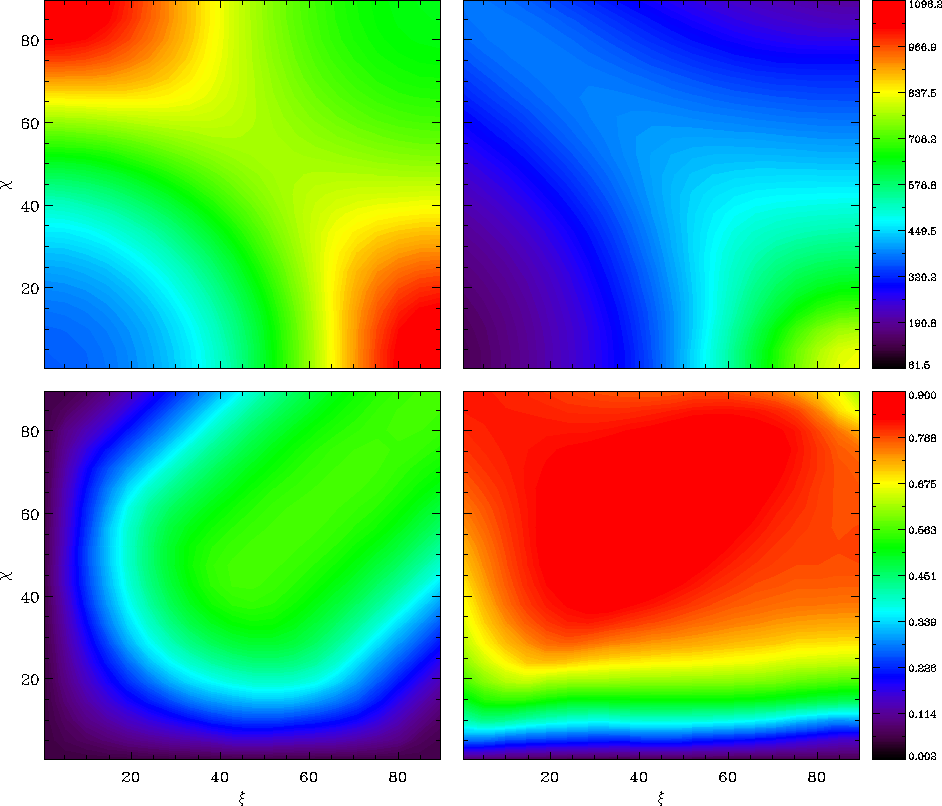
Figure 9: Integrated flux (top row) and pulsed fraction (bottom row) of the radiation emitted from the fireball in the case of model a (left column) and model b (with $\phi_{\mathrm{min}}=100^{\circ}$ and $\phi_{\mathrm{max}}=190^{\circ}$, right column), calculated in the $10$–$50$ keV energy range and plotted as functions of the angles $\chi$ and $\xi$.

In order to account for the effects of quantum electro-dynamics (QED) on the polarization of the emitted radiation, we use the same simplifying approach discussed in Taverna et al. (2015, see also ). Labelling $\ell_{\mathrm{A}}$ and $\ell_{\mathrm{B}}$ the scale-lengths along which the electric field of each photon and the stellar magnetic field evolve, respectively, we divide the region in which photons propagate into two zones: the adiabatic region (characterized by $\ell_{\mathrm{A}}\ll\ell_{\mathrm{B}}$) and the external one (where $\ell_{\mathrm{A}}\gg\ell_{\mathrm{B}}$), sharply separated at the adiabatic radius $r_{\mathrm{a}}$, defined by the equality $\ell_{\mathrm{A}}=\ell_{\mathrm{B}}$. According to this approximation, QED effects ensure that the polarization vector of each photon istantaneously adapts to the local magnetic field direction up to $r_{\mathrm{a}}$, allowing photons to maintain their initial polarization mode. At $r=r_{\mathrm{a}}$ we assume that the photon electric field direction freezes, i.e. it remains oriented in the same direction assumed at the adiabatic radius up to the observer. In this way, in order to reconstruct the polarization properties of the radiation at infinity, the single photon Stokes parameters should be rotated, before to be summed together, by twice the angle $\alpha$ between the local frame $(x,y,z)$ of each photon (with the $z$ axis along the LOS and the $x$ axis perpendicular to the $\boldsymbol{\ell},\boldsymbol{B}$ plane at $r_{\mathrm{a}}$) and the fixed frame $(u,v,w)$ of the polarimeter (with the $w$ axis also along the LOS and $u$, $v$ a generic pair of orthogonal axes perpendicular to $w$, see Taverna et al., 2015, for further details). Generalizing, then, the discrete sum to a continuos photon distribution, we can define the “fluxes” of Stokes parameters as

$$F_{\mathrm{Q}} =\displaystyle{\sum\limits_{j=1}^{2}\int\big{(}n_{\mathrm{X}}-n_{\mathrm{O}}\big{)}\cos(2\alpha)P_{j}\mathrm{d}A_{j}}$$

$$F_{\mathrm{U}} =\displaystyle{\sum\limits_{j=1}^{2}\int\big{(}n_{\mathrm{O}}-n_{\mathrm{X}}\big{)}\sin(2\alpha)P_{j}\mathrm{d}A_{j}}\,,$$ (55)

where the values taken by $\alpha$ depend on the geometrical angles $\chi$ and $\xi$, the rotational phase $\gamma$ and the polar angles $\Theta$ and $\Phi$ that identify the photon emission points in the LOS frame. The Stokes parameter fluxes are finally used to calculate the polarization observables $\Pi_{\mathrm{L}}$ and $\chi_{\mathrm{p}}$, i.e. the linear polarization fraction and the polarization angle, defined as

$$\Pi_{\mathrm{L}} =\dfrac{\sqrt{F^{2}_{\mathrm{Q}}+F^{2}_{\mathrm{U}}}}{F_{\mathrm{I}}}$$

$$\chi_{\mathrm{p}} =\dfrac{1}{2}\arctan\left(\dfrac{F_{\mathrm{U}}}{F_{\mathrm{Q}}}\right)\,.$$ (56)

The intensities $n_{\mathrm{O},\mathrm{X}}$ entering equations (53) and (3.2.3) are taken from the set of models we have computed in advance (see section 3.1). Trilinear interpolation has been used to obtain the intensities at the required values of $B$ and of the polar angles $\theta_{\mathrm{Bk}}$, $\phi_{\mathrm{Bk}}$. In this respect it is useful to notice that the latter are related to the polar angles of the $\boldsymbol{b}_{\mathrm{dip}}$ frame $\theta$, $\phi$ (that can be in turn related to the LOS polar angles $\Theta$, $\Phi$ using equations 3.2.1) by

$$\mu_{\mathrm{Bk}}\equiv\cos\theta_{\mathrm{Bk}} =\boldsymbol{B}\cdot\boldsymbol{\ell}$$

$$\cos\phi_{\mathrm{Bk}} =\bar{\boldsymbol{x}}\cdot\bar{\boldsymbol{\ell}}\,,$$ (57)

where $\bar{\boldsymbol{x}}$ and $\bar{\boldsymbol{\ell}}$ are the unit vectors along the projection of the local normal $\boldsymbol{z}$ (see Appendix A) and $\boldsymbol{\ell}$ in the plane orthogonal to $\boldsymbol{B}$, respectively.

4 Results

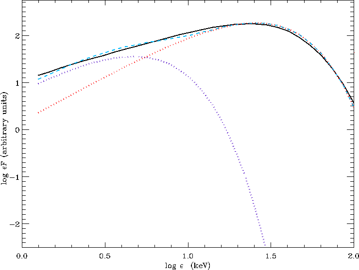
Figure 10: Phase-averaged photon spectrum (black solid line) of the radiation emitted in the case of model b (with $\phi_{\mathrm{min}}=100^{\circ}$ and $\phi_{\mathrm{max}}=190^{\circ}$), fitted by the superposition of two blackbody components for $\chi=60^{\circ}$ and $\xi=30^{\circ}$. The fitting function (58) is marked by the light-blue, dashed line, and the single blackbody components at temperature $T_{1}$ (blue, dotted line) and $T_{2}$ (red, dotted line) are also shown. The results of the fit for different configurations are reported in Table 1.

The intensities calculated in the radiative transfer code and processed in the ray-tracer are then used to obtain the simulated spectra and the polarization observables (both phase-resolved and phase-averaged) as observed at infinity.

Emitting region	$\chi$	$\xi$	$T_{1}$ (keV)	$T_{2}$ (keV)	$A_{2}/A_{1}$
Model a	$60^{\circ}$	$30^{\circ}$	$1.67$	$9.11$	$0.0315$
Model b	$60^{\circ}$	$30^{\circ}$	$1.67$	$9.12$	$0.0315$
Model a	$90^{\circ}$	$0^{\circ}$	$1.67$	$9.18$	$0.0315$
Model b	$90^{\circ}$	$0^{\circ}$	$1.67$	$9.14$	$0.0315$

Table 1: Results of the fits of the phase-averaged total spectrum using the function given by equation (58), for models a and b (the latter characterized by $\phi_{\mathrm{min}}=100^{\circ}$ and $\phi_{\mathrm{max}}=190^{\circ}$) and for different values of the viewing angles $\chi$ and $\xi$ (the case illustrated in Figure 10 is reported in the second row).

4.1 Phase-averaged and phase-resolved spectra

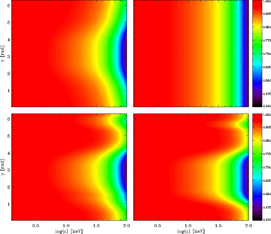
Figure 11: Contour plots of the linear polarization degree $\Pi_{\mathrm{L}}$ as a function of the photon energy $\varepsilon$ and the rotational phase $\gamma$ for $\chi=60^{\circ}$, $\xi=30^{\circ}$ (left-hand column) and $\chi=90^{\circ}$, $\xi=0^{\circ}$ (right-hand column). The top row refers to model a, the bottom row to model b (with $\phi_{\mathrm{min}}=100^{\circ}$ and $\phi_{\mathrm{max}}=190^{\circ}$).

Figure 6 shows the phase-averaged total spectrum of the radiation emitted by the entire torus-shaped fireball (model a) for $\chi=60^{\circ}$ and $\xi=30^{\circ}$ (see Figure 5), compared to those of the ordinary and extraordinary components, separately. The spectrum of the extraordinary photons appears nearly superimposed to the total spectrum at least at lower energies, as already noticed in the case of a single patch (see Figure 3), while ordinary photons give a small contribution only above 30 keV. This confirms that, although the distributions of the O- and X-mode photons at the base of the atmosphere are the same (as mentioned in section 3.1), the radiation collected by an observer at infinity is expected to be polarized essentially in the extraordinary mode. Conversely, the flux of the collected ordinary photons is expected to be much lower than for the extraordinary ones, the ratio $F_{\mathrm{O}}/F_{\mathrm{X}}$ ranging between $\sim 5\times 10^{-3}$ and $0.3$ across the entire $1-100$ keV energy range.

The phase-resolved, total spectrum is instead shown in Figure 7, for $\chi=60^{\circ}$, $\xi=30^{\circ}$ and in the cases of model a (i.e. the same case of Figure 6) and model b with $\phi_{\mathrm{min}}=100^{\circ}$ and $\phi_{\mathrm{max}}=190^{\circ}$ (see the discussion in section 3.2). For the sake of completeness, we also included the case in which the emission from the planar slices at $\phi_{\mathrm{min}}$ and $\phi_{\mathrm{max}}$ is neglected. It is interesting to notice how our simple fireball model is indeed able to reproduce a single-pulse flux profile. In this respect, Figure 8 shows the light curves obtained in the case of model a and model b (with emission from the planar slices at $\phi_{\mathrm{min}}$ and $\phi_{\mathrm{max}}$ included), for two different sets of geometrical angles. In particular, from the left-hand panel it can be clearly seen that pulsations can be obtained, for some favourable viewing geometries, regardless of whether the emitting region is limited or not. This can be explained with the intrinsic anisotropy of the fireball radiation pattern. In fact, as discussed in section 3.1, the photon flux depends on the angle the LOS makes with the local fireball normal (see e.g. Figure 2). Figure 9, which illustrates the integrated flux and pulsed fraction in the $10$–$50$ keV energy range as functions of the angle $\chi$ and $\xi$, further confirms this expectation, showing a wide range of variation for the flux in the $\chi$–$\xi$ plane also in the case of model a, where emission comes from the entire torus. Specifically, it attains its maximum value when the equatorial regions of the fireball enter into view, while it has a minimum when the star is observed along the magnetic axis. On the other hand, the pulsed fraction appears to be much more influenced by the dimension of the emitting region of the torus. Both Figures 8 and 9 show that, for equal $\chi$ and $\xi$, the maximum values of pulsed fraction are attained in the case of model b, where the emitting region is hidden to the observer at certain values of the rotational phase.

Figure 12: Phase-resolved behavior of the polarization angle $\chi_{\mathrm{p}}$ averaged over the entire $1-100$ keV energy range, plotted in the cases of model a (solid lines) and model b with $\phi_{\mathrm{min}}=100^{\circ}$ and $\phi_{\mathrm{max}}=190^{\circ}$ (dashed lines) for different viewing geometries: $\chi=20^{\circ}$, $\xi=10^{\circ}$ (orange), $\chi=60^{\circ}$, $\xi=30^{\circ}$ (red), $\chi=75^{\circ}$, $\xi=15^{\circ}$ (light-blue) and $\chi=90^{\circ}$, $\xi=0^{\circ}$ (violet).

Observations of the “burst forest” emitted by SGR 1900+14 in 2006 (see Israel et al., 2008) suggest that the spectrum of the intermediate flares (and of normal bursts too) is thermal and well reproduced by the superposition of two blackbodies. Although comparing results from our simplified model with observations is premature, we nevertheless attempted to fit the phase-averaged spectra for different values of the geometrical angles $\chi$ and $\xi$ with two blackbody distributions at temperatures $T_{1}$ and $T_{2}$,

$$f(\varepsilon) =A_{1}\varepsilon^{3}\left(\frac{1}{\exp(\varepsilon/kT_{1})-1}+\frac{A_{2}/A_{1}}{\exp(\varepsilon/kT_{2})-1}\right)\,,$$ (58)

where the normalizations $A_{1}$ and $A_{2}$ are related to the emitting areas. As an example, the total emerging spectrum together with the best fit and the single components are shown in Figure 10, for $\chi=60^{\circ}$ and $\xi=30^{\circ}$ and in the case of model b (with $\phi_{\mathrm{min}}=100^{\circ}$ and $\phi_{\mathrm{max}}=190^{\circ}$). Table 1 summarizes the fit parameters obtained for some selected cases. Actually, there is no significant difference switching from model a to model b, and the situation does not appreciably change for different viewing geometries. In general, it turns out that a representation of the model spectra in terms of two blackbodies is satisfactory. With our choice of the temperature distribution (see sections 2.2 and 3.1), $T_{1}$ and $T_{2}$ are $\sim 2$ and $\sim 9$ keV, respectively. Furthermore, the ratio $A_{2}/A_{1}$ between the emitting areas of the harder and the softer components is about $3$% in all the cases considered, translating in a ratio $\sim 0.18$ between the respective blackbody radii. Averaging over a number of different events observed during the burst forest of SGR 1900+14, Israel et al. (2008, see also reference therein) obtained $T_{\mathrm{h}}=9.0\pm 0.3$ keV, $T_{\mathrm{s}}=4.8\pm 0.3$ keV and a ratio $R_{\mathrm{h}}/R_{\mathrm{s}}\sim 0.19\pm 0.03$. Despite the fact that we considered only a single model (with bolometric temperature $T_{\mathrm{b}}=10$ keV and azimuthal extension of the fireball $\phi_{\mathrm{max}}-\phi_{\mathrm{min}}=90^{\circ}$), theoretical predictions appear to be in broad agreement with the observations, although the temperature of the softer component turns out to be somehow lower than the observed one. In this picture, both the blackbody components required to reproduce the observed spectra are essentially made by extraordinary photons (the ordinary ones contributing only at high energies, see Figure 6). This appears at variance with the original suggestion by Israel et al. (2008) that the two components originate from the O- and X-mode photospheres.

4.2 Polarization observables

Figure 13: Phase-averaged linear polarization fraction $\Pi_{\mathrm{L}}$ (top row) and polarization angle $\chi_{\mathrm{p}}$ (bottom row) calculated in the $10$–$50$ keV energy range and plotted as functions of the angles $\chi$ and $\xi$. The left-hand column refers to model a, the right-hand column to model b (with $\phi_{\mathrm{min}}=100^{\circ}$ and $\phi_{\mathrm{max}}=190^{\circ}$).

The observed polarization signal, computed taking into account both vacuum polarization and the geometrical effects due to the magnetic field topology (see Taverna et al., 2015, for further details), confirms that, according to our model, a high degree of polarization is expected for the radiation collected from a magnetar flare.

The behavior of the observed linear polarization fraction, as a function of the rotational phase and photon energy, is shown in Figure 11 for both models a and b and different viewing geometries. In all the cases considered, $\Pi_{\mathrm{L}}$ attains a value generally higher than 80% for photon energies between $1$–$50$ keV. However, radiation appears to be more polarized at lower energies ($\Pi_{\mathrm{L}}>90\%$ for $\varepsilon\sim 1-30$ keV), while the contrary happens above 50 keV, where the polarization degree decreases up to $\sim 40\%$. This behavior, that seems to be opposite to that one would expect considering the dependence of the adiabatic radius $r_{\mathrm{a}}$ on the photon energy (see e.g. Taverna et al., 2015), can be explained looking at the intensity distributions of the ordinary and extraordinary photons (see e.g. Figure 6). In fact, as discussed above, the ratio $F_{\mathrm{O}}/F_{\mathrm{X}}$ increases with the photon energy, justifying the substantial decrease of $\Pi_{\mathrm{L}}$ at higher energies. This is primarily due to the contributions from the patches characterized by smaller magnetic field intensities, for which the O-mode photon flux is larger and comparable to the X-mode one at higher energies (see the left panel of Figure 3). Moreover, the bottom row of Figure 11 shows that a higher degree of polarization is expected when the emission from the planar sides which limit the fireball is considered. Although the difference is actually modest, comparing the bottom-left panel of Figure 11 with the rightmost panels of Figure 7, it appears that the radiation coming from the limiting slices is in general more polarized than that emitted from the remaining part of the torus.

Figure 12 shows the behavior of the polarization angle $\chi_{\mathrm{p}}$ as a function of the rotational phase for both models a and b and different values of the viewing angles $\chi$ and $\xi$. Since, as noted by Taverna et al. (2014, 2015), the polarization angle is essentially constant with the photon energy, in this plot we averaged $\chi_{\mathrm{p}}$ over the entire $1-100$ keV energy range. As in the case of surface emission from a neutron star (Taverna et al., 2015, see also Fernández & Davis 2011; Taverna et al. 2014), the polarization angle oscillates with the rotational phase around a value of $90^{\circ}$, with different amplitudes according to the different values of $\chi$ and $\xi$. This is the expected behavior for photons mainly polarized in the extraordinary mode, as already noticed in section 4.1, with the choice of the polarimeter reference frame made in section 3.2 (see also Taverna et al., 2015). Very small differences are visible between model a (solid lines) and model b (dashed lines) in Figure 12.

As in the case of phase-resolved simulations, also the contour plots in Figure 13, that represent the phase-averaged polarization observables as functions of the angles $\chi$ and $\xi$ in the $10$–$50$ keV energy range, show an overall increase of the polarization fraction moving from model a to model b. The large depolarization that is visible in the top row for certain values of the viewing angles is typical of the dipolar topology of the stellar magnetic field, and it is due to the geometrical effect of rotation of the Stokes parameters from the local frame of each photon to the polarimeter frame (see section 3.2). However, both the patterns of the polarization fraction for model a and b are compatible with radiation highly polarized at the emission, as already noticed by González Caniulef et al. (2016) and Mignani et al. (2017) in the case of blackbody or atmospherical emission from the star. Finally, also the behavior of the phase-averaged polarization angle is that expected for radiation characterized by an excess of extraordinary photons.

5 Discussion and conclusions

We have revisited the problem of modeling the spectral and polarization properties of the radiation emitted during magnetar flares in the context of the trapped-fireball model (see Thompson & Duncan, 1995, 2001). Our code integrates the radiative transfer equations for both ordinary and extraordinary photons in the fireball atmospheric layer, divided in a number of different patches. This model generalizes the approach presented by Lyubarsky (2002), who treated the problem in the one dimensional approximation by solving the radiative transfer equation for X-mode photons only, and in the case of $\boldsymbol{B}$ parallel to the patch normal. The outputs of the radiative transfer code have been then reprocessed through a ray-tracing code (see section 3.2), in order to obtain the spectra and the polarization observable distributions as measured by a distant observer. Radiation has been assumed to come from either the entire torus-like fireball or a portion limited in the azimuthal direction between two values $\phi_{\mathrm{min}}$ and $\phi_{\mathrm{max}}$. In the latter case, also emission from the two planar slices at the boundaries has been accounted for. The contributions from the patches which enter into view are finally summed together, providing the photon fluxes in the two normal modes as functions of energy, rotational phase and the two angles $\chi$ and $\xi$ which characterize the viewing geometry. The Stokes parameter fluxes are also computed, taking into account the effects of both vacuum polarization and Stokes parameter rotation (see section 3.2.3). The polarization properties of the radiation, i.e. the linear polarization fraction and the polarization angle are finally obtained for both phase-averaged and phase-resolved simulations.

5.1 Second-order processes

Throughout this paper, we considered magnetic Thomson scattering as the dominant source of opacity in the plasma. However, other second-order processes could be potentially relevant when strong magnetic fields are considered. In section 2.2 we mentioned the role of double-Compton scattering in ensuring local thermal equilibrium at large optical depths deep in the fireball. Here we discuss the role of additional processes, such as thermal bremsstrahlung and photon splitting.

Since we considered non-relativistic particles ($kT\ll m_{\mathrm{e}}c^{2}$), electron-electron (positron-positron) bremsstrahlung turns out to be negligible. In fact, its contribution vanishes in the dipole approximation and it starts to be important only in the relativistic limit, at particle energies $\ga 300$ keV (the cross section is $\sim 2$ orders of magnitude smaller than the Thomson cross section at $\varepsilon\sim 10$ keV, see Haug, 1975). Actually, in a pair plasma, where both electrons and positrons have comparable densities, the dominant contribution comes from electron-positron bremsstrahlung Svensson (1982); Haug (1985a). Unfortunately, no complete treatment of this process in a strong magnetic field is currently available in the literature. Some considerations on its importance relative to scattering can nevertheless be made. In the free-field case, electron-positron emissivity is only slightly enhanced with respect to the electron-proton one (by a factor $\sim 2^{3/2}$; Svensson, 1982). The cross section is $\sim 0.5\,\sigma_{\mathrm{T}}$, at $\varepsilon=1$ keV and $kT=10$ keV, and decreases for both increasing photon and particle energy (see Haug, 1985b). Electron-proton bremsstrahlung has been investigated also in the strong-field limit by Lieu (1981, see also ), who showed that the cross section for the extraordinary photons is strongly suppressed with respect to that for the O-mode, which, in turn, shows a behavior similar to that of the free-field limit. Assuming that Svensson (1982) result remains valid also at $B\ga B_{\mathrm{Q}}$, electron-positron bremsstrahlung cross section is likely to be smaller than the electron scattering one for both the ordinary and the extraordinary modes.

Photon splitting, on the other hand, can affect the photon spectra in a wide range of energies (see e.g. Adler et al., 1970; Adler, 1971). The effects of this process, however, change radically according to the intensity of the magnetic field in which photons propagate, and the splitting of a photon in more than two photons is suppressed for $B\la B_{\mathrm{Q}}$ Bialynicka-Birula & Bialynicki-Birula (1970). The expression for the photon splitting probability, that strongly depends on the polarization mode of the photons involved, has been discussed by Stoneham (1979, see also ) in the weak-field limit and for low energies ($\varepsilon\ll m_{\mathrm{e}}c^{2}$). In particular, taking into account weak dispersive effects, the only allowed channel turns out to be that of an X-mode photon splitting in two O-mode photons. The maximum absorption coefficient of the process results

$$\alpha_{\mathrm{sp}}(\mathrm{X}\rightarrow\mathrm{OO}) =-\frac{\alpha_{\mathrm{F}}^{3}m_{\mathrm{e}}c}{60\pi^{2}\hbar}\left(\frac{B\sin\theta_{\mathrm{Bk}}}{B_{\mathrm{Q}}}\right)^{6}\left(\frac{\varepsilon}{m_{\mathrm{e}}c^{2}}\right)^{5}$$

$$\,\,\,\,\,\,\,\times\left[M_{1}(B/B_{\mathrm{Q}})\right]^{2}\,,$$ (59)

where the complete expression of the function $M_{1}(B/B_{\mathrm{Q}})$ is given in Stoneham (1979). The dependencies on magnetic field and photon energy in equation (5.1) make clear that the effects of photon splitting are quite modest for photons with energies $1$–$100$ keV (the range of interest in this work) and for weak magnetic fields. On the other hand, although for super-critical fields one should consider also the contribution that comes from the splitting of a photon in more than two photons, the amplitude of the process goes as $\exp(-B/B_{\mathrm{Q}})$ Stoneham (1979). A simple numerical estimate shows that the absorption coefficient associated to electron (positron) scattering $\alpha_{\mathrm{sc}}=n_{\mathrm{e}}\sigma_{\mathrm{T}}$ typically exceeds the coefficient $\alpha_{\mathrm{sp}}$ by more than a factor $\sim 3$ even at the highest photon energy we considered ($\varepsilon=100$ keV).

5.2 Spectral analysis

We presented the results of theoretical simulations for a template source endowed with a dipolar magnetic field, with polar intensity $B_{\mathrm{p}}=2\times 10^{14}$ G. As it can be seen in Figure 6, the dominant contribution to the total spectrum comes from extraordinary photons, the ordinary photon flux being in general one order of magnitude (or more) smaller. This clearly follows from the fact that O-mode and X-mode photons have different scattering opacities, as discussed in section 2.1. The cross section for extraordinary photons is strongly supressed, by a factor $(\varepsilon/\varepsilon_{\mathrm{B}})^{2}$, with respect to that of ordinary ones. Nevertheless, as illustrated in Figure 3, O-mode photon contribution appears to increase at high energies ($\varepsilon\ga 50$ keV), as well as for lower magnetic field intensities, while the spectrum of X-mode ones is practically unchanged by varying the magnetic field strength. This suggests, in particular, that more energetic ordinary photons escape the fireball preferably far from the star surface, where the magnetic field is weaker, contrary to extraordinary ones. We found that the total spectrum can be well reproduced in terms of the superposition of two thermal components, in agreement with the results obtained by Israel et al. (2008) in their study of the intermediate flares emitted during the SGR 1900+14 burst forest. We note that, although we considered only one illustrative case, corresponding to a bolometric temperature $T_{\mathrm{b}}=10$ keV and an angular opening $\phi_{\mathrm{max}}-\phi_{\mathrm{min}}=90^{\circ}$, the temperatures and emitting area ratio we obtained for the two fitting components are compatible with observations. However, our results do not appear to support the suggestion by Israel et al. (2008) according to which the soft and hard blackbodies are associated to photons coming from the O-mode and X-mode photospheres, respectively, as one can easily verify comparing Figures 6 and 10. The presence of two components in the spectral fit comes rather from the broad distrubution of X-mode photons, which, according to their energy, escape the fireball atmosphere at different depths, where the temperature attains different values. This causes a flattening of the number flux at lower energies ($\varepsilon\la kT_{\mathrm{b}}$), as already noted by Lyubarsky (2002) and clearly visible in Figure 3.

Our model can also reproduce the pulsations observed in intermediate/giant flare decay tails. Actually, this problem has been extensively addressed by van Putten et al. (2016), who investigated, in particular, the geometry of the magnetar flare beaming, driven by relativistic outflows of charged particles Thompson & Duncan (1995, 2001). According to their model, it is indeed the presence of these outflows that allows to explain the rotational modulation of the observed light curves as expected from the time evolution of the trapped fireball. They noted that, contrary of what observations show, the light curve modulation would change dramatically as the fireball shrinks, if only a localized emission region on the torus (and no beaming) is considered. However, the study of the time evolution of magnetar flares and how this can influence the shape of the light curves is outside the aims of our work. For this reason, in our model we focused only on the properties of the radiation emitted from a steady trapped-fireball, neglecting all the possible contributions coming from the advection of baryons due to relativistic outflows. Under these conditions, we found that our model is able to account for the pulsations observed in the decay tails of intermediate/giant flares, independently on whether the emitting region of the torus-shaped fireball is limited azimuthally (model b) or not (model a). The shape of the light curve and the pulsed fraction depend clearly on the viewing angles $\chi$ and $\xi$, as well as on the angular opening $\phi_{\mathrm{max}}-\phi_{\mathrm{min}}$ in the case of model b, as shown in Figure 8 and in the bottom row of Figure 9. Moreover, a certain degree of beaming turns out to be present also in our model, as visible e.g. in the angular distributions plotted in Figure 2 (which show that ordinary photons are preferentially emitted along the local magnetic field direction) and in the top row of Figure 9.

5.3 Polarization properties

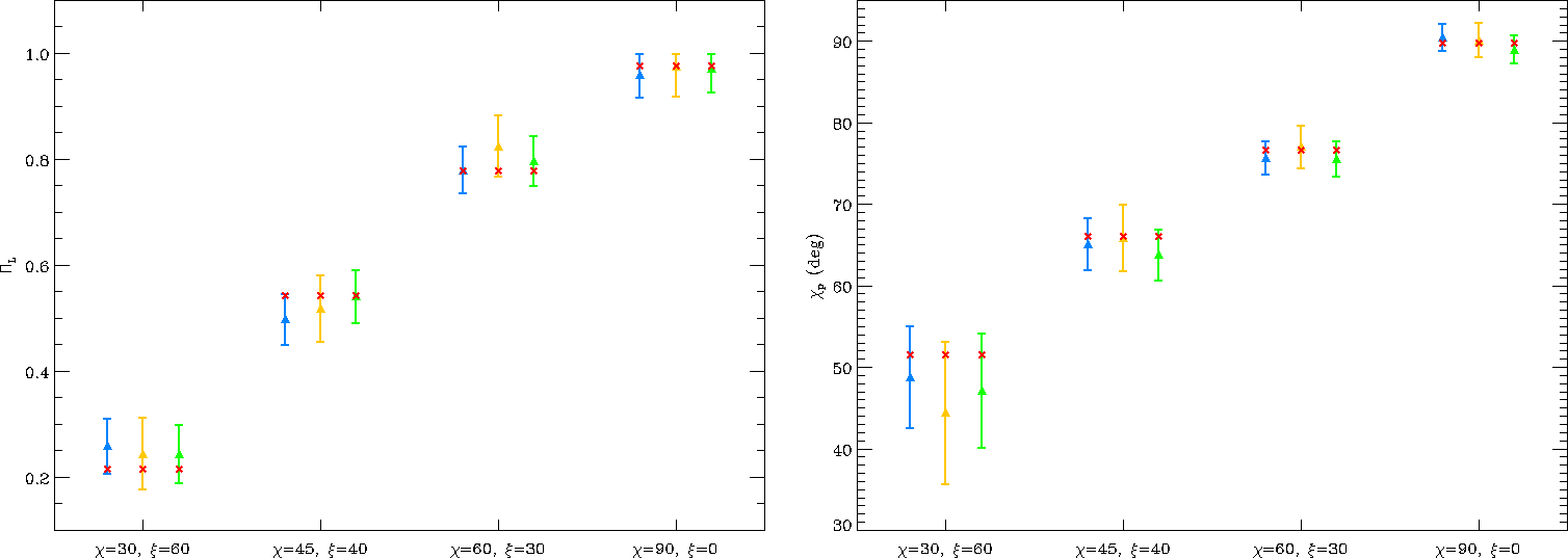
Figure 14: Simulations of the phase-averaged response (triangles with error bars) of the XIPE (blue), IXPE (orange) and eXTP (green) polarimeters to the signal predicted by our theoretical model (in the case of model b) for an exposure time $t_{\mathrm{exp}}=1.737$ s, X-ray flux $F_{\mathrm{X}}=4.68\times 10^{-7}$ erg cm^-2 s^-1 in the $1$–$10$ keV energy range and different viewing geometries (red crosses). The instrument specifications correspond to the respective baseline configurations.

Our work relies on the assumption that the plasma contributions to the dielectric tensor are negligible with respect to the vacuum terms. For this reason we did not consider vacuum resonance (see e.g. Lai & Ho, 2003), that occurs when plasma and vacuum contributions are comparable and influences the observed polarization signal switching the photon modes at an energy close to the resonant energy (see Lyubarsky, 2002),

$$\varepsilon_{\mathrm{vr}} =\sqrt{6}m_{\mathrm{e}}c^{2}\bigg{(}\frac{2\pi T}{m_{\mathrm{e}}c^{2}}\bigg{)}^{1/4}\exp\bigg{(}-\frac{m_{\mathrm{e}}c^{2}}{2T}\bigg{)}\,,$$ (60)

where $T$ is given by equation (23). According to the original model by Thompson & Duncan (1995), plasma effects in the fireball are essentially due to electron-positron pairs. The baryonic component inside the fireball is indeed much less important, since baryons are mostly advected away from the star surface through relativistic outflows (see van Putten et al., 2016). However, even at large optical depths, where the pair density is higher, the resonance energy results rather low ($\sim 1$ keV). This ensures that, over the entire $1$–$100$ keV energy range we considered, vacuum resonance can be safely neglected, assuming vacuum effects dominant over the plasma ones. Furthermore, the possible residual presence of baryons in the fireball is not even expected to modify photon polarization through scattering, since the (Thomson) cross sections for photon scatterings onto baryons are suppressed with respect to those for scatterings onto pairs by a factor $\sim 10^{-6}$. We note also that the possible effects of resonant scattering onto protons, which occurs at the cyclotron energy $E_{\mathrm{cp}}=0.63(B/10^{14}\,\mathrm{G})$ keV, are not going to affect the spectrum and the polarization properties in the energy range we considered. In fact, for a polar magnetic field $B_{\mathrm{p}}=2\times 10^{14}$ G, it is $E_{\mathrm{cp}}\la 1$ keV.

In the code both vacuum polarization effects and Stokes parameter rotation are accounted for (see section 3.2.3). We assumed that the adiabatic radius $r_{\mathrm{a}}$ is a sharp edge separating the adiabatic region (where the photon polarization vectors are locked to the star magnetic field direction) from the external region (where the polarization vector direction is frozen). Our results strongly indicate that magnetar flare radiation is highly polarized and dominated by extraordinary photons. In fact, as illustrated in the phase-resolved plots of Figure 11, the linear polarization degree attains values higher than $80\%$ over almost all the entire $1$–$100$ keV energy range, dropping to about $70\%$ only at the highest energies. This decrease in $\Pi_{\mathrm{L}}$ is compatible with the increase of the ordinary photon contribution at higher energies we discussed in the previous section. Moreover, when an azimuthally limited emitting region is considered, radiation collected from the planar slices at the boundaries results in general even more polarized than the radiation with the same energy coming from the torus.

As already pointed out in Taverna et al. (2015), phase-averaged simulations show more clearly the depolarizing effects of Stokes parameter rotation (see Figure 13). This is essentially due to the fact that instruments give information about the Stokes parameters of each collected photon. Due to the Stokes parameter rotation at the adiabatic radius, the average over the star rotational period generally reduce the observed polarization degree with respect to what one would see in a phase-resolved measurement, except for some favourable viewing geometries. In particular, the maximum $\Pi_{\mathrm{L}}$ (here nearly $100\%$) is attained for $\chi=90^{\circ}$, $\xi=0^{\circ}$, i.e. the case of an aligned rotator seen perpendicularly to the magnetic axis, where the effects of rotation are less important. Such a polarization signal is strong enough to be readily measurable by the new-generation, X-ray polarimeters currently under development. A plot of the simulated, phase-averaged response of XIPE, IXPE and eXTP to the signal predicted by our model, observed at different viewing geometries, is shown in Figure 14. Here we refer to an event characterized by an X-ray flux $F_{\mathrm{X}}=4.68\times 10^{-7}$ erg cm^-2 s^-1 in the $1$–$10$ keV energy range and an exposure time $t_{\mathrm{exp}}=1.737$ s, i.e. the values tabulated by Israel et al. (2008) for the intermediate flare labelled IF1. Both polarization fraction and angle measurements recover the values expected from the theoretical model with an acceptable degree of accuracy (within 1 sigma). It can be noted that, while the errors on the polarization fraction are more or less the same for all the geometrical configurations considered, those on the polarization angle increase by decreasing the corresponding polarization degree. For $\Pi_{\mathrm{L}}\la 20\%$, polarization angle measurements turn out to be dominated by instrumental effects. In principle, polarization angle estimates could be useful to understand in which mode the collected radiation is polarized. However, as noted in previous works (see e.g. Taverna et al., 2015; González Caniulef et al., 2016; Mignani et al., 2017), it should be taken into account that a polarization analysis alone does not suffice to this aim. In fact, the value of the polarization angle returned by the polarimeter depends on the orientation of its reference axis with respect to the projection of the star spin axis on the plane of the sky, that is a priori unknown. Nevertheless, as tested in the case of persistent emission (see Taverna et al., 2014), also for magnetar flares the oscillatory behavior of the polarization angle as a function of the rotational phase can be used to constrain the values of the viewing angles $\chi$ and $\xi$ (see Figure 12).

Yang & Zhang (2015) have recently presented a model to investigate the polarization properties of the radiation emitted during magnetar flare pulsating tails. They calculated the radiative transfer in the fireball atmosphere using Monte Carlo simulations, in which they fixed the number of photons (5000) in two energy bands ($1$–$30$ keV and $30$–$100$ keV), assumed the star is an aligned rotator and collected photons for different inclination of the LOS with respect to the magnetic axis. QED effects were also considered in the “sharp-edge” approximation, as we did. While starting from the same initial conditions as in our work, their polarization fraction turns out to be quite modest, contrary to our findings. In fact, even if the collected radiation results mostly polarized in the extraordinary mode for all the considered viewing geometries, they obtained $\Pi_{\mathrm{L}}=30\%$ in the softer band (and only $10\%$ in the harder one) when the LOS is perpendicular to the magnetic axis, namely the configuration which should produce the largest phase-averaged polarization degree. van Putten et al. (2016) used as well a Monte Carlo code, fixing instead the computational time dedicated to each run rahter than the photon number. Although a complete analysis in this sense is outside their scopes, they also explored the polarization spectrum of the magnetar flare emission, finding that the ratio between ordinary and extraordinary photon intensities strongly depends on the outflow velocity. However, radiation appears to be largely dominated by ordinary photons, the two intensities becoming comparable only at high particle velocities ($\ga 0.8\,c$) and only for certain inclinations between the LOS and the magnetic axis. This could be explained by the fact that O-mode photons are tightly-coupled to the plasma deep in the fireball due to their large scattering opacity, so that they can be more easily advected by the relativistic outflow than X-mode one. Basically, in the case of sources for which an independent method to constrain the direction of the source rotation axis is possible, a polarization angle measurement can definitively disambiguate what polarization mode dominates the collected radiation, allowing to evaluate the actual role of relativistic outflows in characterizing magnetar flare emission.

Appendix A Local normal to the fireball surface

Given a point $P$ on the fireball surface, characterized by the position vector

$$\boldsymbol{m}(\theta,\phi) =r\left(\begin{array}[]{c}\sin\theta\cos\phi\\ \sin\theta\sin\phi\\ \cos\theta\end{array}\right)=R_{\mathrm{max}}\left(\begin{array}[]{c}\sin^{3}\theta\cos\phi\\ \sin^{3}\theta\sin\phi\\ \sin^{2}\theta\cos\theta\end{array}\right)\,,$$ (67)

where $\theta$ and $\phi$ are related to $\Theta$ and $\Phi$ by equations (3.2.1) and equation (31) has been used, the surface normal $\boldsymbol{z}$ can be derived as

$$\boldsymbol{z} =\frac{\boldsymbol{m}_{\theta}\times\boldsymbol{m}_{\phi}}{|\boldsymbol{m}_{\theta}\times\boldsymbol{m}_{\phi}|}\,,$$ (68)

with

$$\boldsymbol{m}_{\theta} =\frac{\partial\boldsymbol{m}}{\partial\theta},\,\,\,\,\,\,\boldsymbol{m}_{\phi}=\frac{\partial\boldsymbol{m}}{\partial\phi}\,.$$ (69)

Starting from equation (67) and after some algebra one obtains the components of $\boldsymbol{z}$ in the $\boldsymbol{b}_{\mathrm{dip}}$ frame,

$$\boldsymbol{z} =\frac{1}{\sqrt{1+3\cos^{2}\theta}}\left(\begin{array}[]{c}(1-3\cos^{2}\theta)\cos\phi\\ (1-3\cos^{2}\theta)\sin\phi\\ 3\sin\theta\cos\theta\end{array}\right)\,.$$ (73)

Appendix B Domain of the fireball terminator

The complete solution of the inequality (42) is given by the intersection of the solutions of $A<1$ and $A>-1$, where $A=3\sin\theta\cos\theta\cos\eta/[\sin\eta(3\cos^{2}\theta-1)]$. Solving for $\theta$ the two equations $A=\pm 1$, one finds four distinct roots

$$t_{++} \equiv\frac{3\cos\eta+\sqrt{\cos^{2}\eta+8}}{2\sin\eta}\,;\,\,\,t_{+-}\equiv\frac{3\cos\eta-\sqrt{\cos^{2}\eta+8}}{2\sin\eta}$$

$$t_{-+} \equiv-t_{+-}\,;\,\,\,\,\,\,\,\,\,\,\,\,\,\,\,\,\,\,\,\,\,\,\,\,\,\,\,\,\,\,\,\,\,\,\,\,\,\,\,\,\,\,\,\,\,t_{--}\equiv-t_{++}\,.$$

In particular, solving separately $A<1$ and $A>-1$ leads to

$$0<\theta<\mathrm{min}_{-+}^{(1)}\,\cup\,\,\mathrm{max}_{-+}^{(1)}<\theta<\mathrm{min}_{--}^{(2)}\,\cup\,$$

$$\mathrm{max}_{--}^{(2)}<\theta<\pi$$ (75)

and

$$0<\theta<\mathrm{min}_{++}^{(1)}\,\cup\,\,\mathrm{max}_{++}^{(1)}<\theta<\mathrm{min}_{+-}^{(2)}\,\cup\,$$

$$\mathrm{max}_{+-}^{(2)}<\theta<\pi\,,$$ (76)

respectively, where we defined

$$\begin{array}[]{l}\mathrm{min}_{\pm\pm}^{(1)}\,\equiv\min\left[\arctan(t_{\pm\pm}),\dfrac{1}{2}\arccos\left(-\dfrac{1}{3}\right)\right]\\ \\ \mathrm{max}_{\pm\pm}^{(1)}\equiv\max\left[\arctan(t_{\pm\pm}),\dfrac{1}{2}\arccos\left(-\dfrac{1}{3}\right)\right]\\ \\ \mathrm{min}_{\pm\pm}^{(2)}\,\equiv\min\left[\pi+\arctan(t_{\pm\pm}),\pi-\dfrac{1}{2}\arccos\left(-\dfrac{1}{3}\right)\right]\\ \\ \mathrm{max}_{\pm\pm}^{(2)}\equiv\max\left[\pi+\arctan(t_{\pm\pm}),\pi-\dfrac{1}{2}\arccos\left(-\dfrac{1}{3}\right)\right]\,.\end{array}$$ (84)

In order to compute the intersection of the two solutions (B) and (B), it is necessary to sort the quantities given in (84) in increasing order,

$$(a_{1},a_{2},a_{3},a_{4}) \equiv\tt{sort}(\mathrm{min}_{-+}^{(1)},\mathrm{min}_{++}^{(1)},\mathrm{max}_{-+}^{(1)},\mathrm{max}_{++}^{(1)})$$

$$(b_{1},b_{2},b_{3},b_{4}) \equiv\tt{sort}(\mathrm{min}_{--}^{(2)},\mathrm{min}_{+-}^{(2)},\mathrm{max}_{--}^{(2)},\mathrm{max}_{+-}^{(2)})\,.$$ (85)

In this way, one can write the ranges of $\theta$ for which the terminator exists,

$$\theta_{\mathrm{min}}<\theta<a_{1}\,\cup\,a_{2}<\theta<a_{3}\,\cup\,a_{4}<\theta\leq\pi/2\,\cup$$

$$\pi/2<\theta<b_{1}\,\,\,\cup\,b_{2}<\theta<b_{3}\,\,\cup\,b_{4}<\theta<\theta_{\mathrm{max}}\,.$$ (86)

Actually, it can be shown that the two intervals $a_{2}<\theta<a_{3}$ and $b_{2}<\theta<b_{3}$ are present if and only if $a_{2}=\mathrm{max}_{\pm+}^{(1)}$ and $b_{2}=\mathrm{max}_{\pm-}^{(2)}$.

Appendix C Coordinate transformation between the $\boldsymbol{b}_{\mathrm{dip}}$ and the LOS reference frames

Given a vector $\boldsymbol{v}$ with components $(v_{p},v_{q},v_{t})$ in the $\boldsymbol{b}_{\mathrm{dip}}$ reference frame, its components $(v_{X},v_{Y},v_{Z})$ in the LOS frame are given by the following change-of-basis transformation:

$$v_{X} =v_{p}p_{X}+v_{q}q_{X}+v_{t}t_{X}$$

$$v_{Y} =v_{p}p_{Y}+v_{q}q_{Y}+v_{t}t_{Y}$$

$$v_{Z} =v_{p}p_{Z}+v_{q}q_{Z}+v_{t}t_{Z}\,,$$ (87)

where the components of the unit vectors $\boldsymbol{p}$, $\boldsymbol{q}$ and $\boldsymbol{t}$ in the LOS frame are given in equations (3.2.1).

References

- Adler (1971) Adler S. L., 1971, Ann. Phys., NY 67, 599
- Adler et al. (1970) Adler S. L., Bahcall J. N., Callan C. G., Rosenbluth M. N., 1970, Phys. Rev. Lett., 25, 1061
- Alexander et al. (1989) Alexander S. G., Mészáros P., Bussard R. W., 1989, ApJ, 342, 928
- Alexander & Mészáros (1991) Alexander S. G., Mészáros P., 1991, ApJ, 372, 554
- Bialynicka-Birula & Bialynicki-Birula (1970) Bialynicka-Birula Z., Bialynicka-Birula I., 1970, Phys. Rev. D., 2, 2341
- Braithwaite (2009) Braithwaite J., 2009, MNRAS, 397,763
- Bulik (1998) Bulik T., 1998, Acta Astronomica, 48, 695
- Duncan & Thompson (1992) Duncan R. C., Thompson C., 1992, ApJ, 392, L9
- Elenbass et al. (2016) Elenbaas C., Watts A. L., Turolla R., Heyl J. S., 2016, MNRAS, 456, 3282
- Fernández & Davis (2011) Fernández R., Davis S. W., 2011, ApJ, 730, 131
- Feroci et al. (2004) Feroci M., Caliandro G. A., Massaro E., Mereghetti S., Woods P. M., 2004, ApJ, 612, 408
- Gnedin & Pavlov (1974) Gnedin Yu. N., Pavlov G. G., 1974, Soviet Phys.-JETP Lett., 38, 903
- González Caniulef et al. (2016) González Caniulef D., Zane S., Taverna R., Turolla R., Wu K., 2016, MNRAS, 459, 3585
- Harding & Lai (2006) Harding A. K., Lai D., 2006, Rep. Prog. Phys., 69, 2631
- Haug (1975) Haug E., 1975, Zeitschrift Naturforschung Teil A, 30, 1099
- Haug (1985a) Haug E., 1985a, A&A, 148, 386
- Haug (1985b) Haug E., 1985b, Phys. Rev. D, 31, 2120
- Heisemberg & Euler (1936) Heisemberg W., Euler H., 1936, Zeitschrisft für Physik, 98, 714
- Herold (1979) Herold H., 1979, Phys. Rev. D, 19, 2868
- Heyl & Shaviv (2002) Heyl J. S., Shaviv N. J., 2002, Phys. Rev. D, 66, 023002
- Ho & Lai (2003) Ho W. C. G., Lai D., 2003, MNRAS, 338, 233
- Israel et al. (2008) Israel G. L. et al., 2008, ApJ, 685, 1114
- Lai & Ho (2003) Lai D., Ho W. C. G., 2003, ApJ, 588, 962
- Lai et al. (2010) Lai D., Ho W. C. G., van Adelsberg M., Wang C., Heyl J. S., 2010, X-ray Polarimetry: A New Window in Astrophysics. Cambridge Univ. Press, Cambridge
- Lauer et al. (1983) Lauer J., Herold H., Ruder H., Wunner G., 1983, J. Phys. B: At. Mol. Phys., 16, 3673
- Lieu (1981) Lieu R., 1981, Ap. & Sp. Sci., 80, 157
- Lightman (1981) Lightman A., 1981, ApJ, 244, 392
- Lyubarsky (2002) Lyubarsky Y. E., 2002, MNRAS, 332, 199
- Lyutikov (2003) Lyutikov M., 2003, MNRAS, 346, 540
- Mereghetti (2008) Mereghetti S., 2008, A&A Rev., 15, 225
- Mészáros et al. (1989) Mészáros P., Pavlov G. G., Shibanov Yu. A., 1989, ApJ, 337, 426
- Mészáros (1992) Mészáros P., 1992, High-Energy Radiation from Magnetized Neutron Stars. Univ. Chicago Press, Chicago
- Mignani et al. (2017) Mignani R. P., Testa V., González Caniulef D., Taverna R., Turolla R., Zane S., Wu K., 2017, MNRAS, 465, 492
- Nobili, Turolla & Zane (2008) Nobili L., Turolla R., Zane S., 2008, MNRAS, 386, 1527
- Olive et al. (2004) Olive J.-F. et al., 2004, ApJ, 616, 1148
- Perna & Pons (2011) Perna R., Pons J. A., 2011, ApJ, 727, L51
- Pomraning (1973) Pomraning G. C., 1973, The equations of radiation hydrodynamics. Dover publications inc. Mineola, New York
- Soffitta (2016) Soffitta P. et al., 2016, Proc. SPIE, 9905, 990515
- Stoneham (1979) Stoneham R. J., 1979, J. Phys. A, 12, 2187
- Svensson (1982) Svensson R., 1982, ApJ, 258, 335
- Taverna et al. (2014) Taverna R., Muleri F., Turolla R., Soffitta P., Fabiani S., Nobili L., 2014, MNRAS, 438, 1686
- Taverna et al. (2015) Taverna R., Turolla R., González Caniulef D., Zane S., Muleri F., Soffitta P., 2015, MNRAS, 454, 3254
- Thompson & Duncan (1995) Thompson C., Duncan R. C., 1995, MNRAS, 275, 255
- Thompson & Duncan (2001) Thompson C., Duncan R. C., 2001, ApJ, 561, 980
- Thompson et al. (2002) Thompson C., Lyutikov M., Kulkarni S. R., 2002, ApJ, 574, 332
- Turolla et al. (2015) Turolla R., Zane S., Watts A. L., 2015, Rep. Prog. Phys., 78, 11
- van Putten et al. (2016) van Putten T., Watts A. L., Baring M. G., Wijers R. A. M. J., 2016, MNRAS, 461, 877
- Ventura (1979) Ventura J., 1979, Phys. Rev. D, 19, 1684
- Weisskopf et al. (2013) Weisskopf M. et al., 2013, Proc. SPIE, 8859, 885908
- Woods et al. (2005) Woods P. M. et al., 2005, ApJ, 629, 985
- Yang & Zhang (2015) Yang Y. P., Zhang B., 2015, ApJ, 815, 45
- Zane & Turolla (2006) Zane S., Turolla R., 2006, MNRAS, 366, 727
- Zhang et al. (2016) Zhang S. N. et al., 2016, Proc. SPIE, 9905, 99051Q