Analysis, simulation and optimal control
of a SEIR model for Ebola virus
with demographic effects

Abstract.

Ebola virus is one of the most virulent pathogens for humans. We present a mathematical description of different Susceptible–Exposed–Infectious–Recovered (SEIR) models. By using mathematical modeling and analysis, the latest major outbreak of Ebola virus in West Africa is described. Our aim is to study and discuss the properties of SEIR models with respect to Ebola virus, the information they provide, and when the models make sense. We added to the basic SEIR model demographic effects in order to analyze the equilibria with vital dynamics. Numerical simulations confirm the theoretical analysis. The control of the propagation of the virus through vaccination is investigated and the case study of Liberia is discussed in detail.

1. Introduction

Ebola is a deadly virus that attacks healthy cells and replicates itself in a host’s body. The virus, previously known as Ebola hemorrhagic fever, is the deadliest pathogen for humans and has recently affected several African countries. Discovered in 1976 in Central Africa, the recent outbreaks affected the more heavily populated countries of West Africa [5, 36]. Early symptoms of Ebola include: fever, headache, joint and muscle aches, sore throat, and weakness. Later symptoms include diarrhea, vomiting, stomach pain, hiccups, rashes, bleeding, and organ failure. When Ebola progresses to external and internal bleeding, it is almost always fatal [1, 22, 31, 37, 39]. Ebola virus is transmitted initially to human by contact with an infected animal’s body fluid. Ebola is most commonly spread by contact with blood and secretions, either via direct contact (through broken skin or mucous membranes in, e.g., the eyes, nose, or mouth) with the infected individual or fluids on clothing or other surfaces, as well as needles [8, 11, 14, 25, 35].

Epidemic models date back to the early twentieth century, to the 1927 work by Kermack and McKendrick, whose models were used to study the plague and cholera epidemics [19, 20]. Epidemic modeling is nowadays a powerful tool for investigating human infectious diseases, such as Ebola, contributing to the understanding of the dynamics of virus, providing useful predictions about the potential transmission of the virus and the effectiveness of possible control measures, which can provide valuable information for public health policy makers [12, 16, 21, 23, 33, 34].

The most commonly implemented models in epidemiology are the SIR and SEIR models. The SIR model consists of three compartments: Susceptible individuals $S$, Infectious individuals $I$, and Recovered individuals $R$. In many infectious diseases there is an exposed period after the transmission of the infection from susceptible to potentially infective members, but before these potential infective can transmit infection. Then an extra compartment is introduced, the so called exposed class $E$, and we use compartments $S$, $E$, $I$ and $R$ to give a generalization of the basic SIR model [10]. When analyzing a new outbreak, researchers usually start with the basic SIR and SEIR models to fit the available outbreak data, obtaining estimates for the parameters of the model. Only after that, more complicated models may be considered [10]. In case of Ebola, the SIR model has already been deeply explored in the literature [26, 27]. For a case study of the Ebola virus in Guinea, through a SIR model, we refer to [28]. The results obtained by SIR models are good enough, taking into account their simplicity. However, the transmission of Ebola virus is better described by a SEIR model. This is because it takes a certain time for an infected individual to become infectious. During that period of time, such individuals are in the exposed/latent compartment. A mathematical description of the spread of Ebola virus based on the basic SEIR model has been carried out, e.g. in [24, 29]. Discrete SEIR time models to Ebola epidemics are available in [6]. In our work, we are interested in continuous time models, which are more common with respect to Ebola modeling [2, 9, 24]. In [2], the homotopy decomposition method is used to solve a system of equations modeling Ebola hemorrhagic fever involving the so called beta derivative, which can be considered as the fractional order of the system. In our case, we deal with classical derivatives and standard integer-order systems. For fractional modeling of Ebola, see also [3]. Our main control measure for the propagation of the virus is vaccination. For the use of quarantine as a control measure to limit the transmission of the Ebola virus using a SEIR model, we refer the interested reader to [9]. For a comparison study between the basic SIR and SEIR models to describe an Ebola outbreak, and for the conclusion of superiority of the SEIR model, we refer the reader to [30]. It turns out that in available Ebola studies with SEIR models, the population is assumed to be constant: see Remark 1 of [29] and Proposition 2.2 of [30]. This assumption is far from being true in West African countries. For example, in Liberia, the birth rate is approximately four times the death rate [18]. Motivated by this fact, here our main aim is to study the latest major outbreak of Ebola virus occurred in Liberia through an appropriate SEIR model with vital dynamics, which takes into account the demographic effects on the population. This is in contrast with all available results in the literature.

The paper is organized as follows. In Section 2, we recall the basic mathematical SEIR model to describe the dynamics of the Ebola virus that recently affected West Africa. After the modeling, we analyze mathematically the SEIR model. In Section 3, we propose and analyze a new SEIR model with vital dynamics by adding demographic effects (Section 3.1). The equilibria of the model are studied in Section 3.2. Then, a numerical simulation is presented, which confirms the theoretical analysis (Section 3.3). After numerical resolution of the model, in Section 4 we control the propagation of the virus through vaccination, reducing the number of infected individuals while taking into account the cost of vaccination. Finally, in Section 5, we propose and investigate a more general model with demographic effects, for which there is an increase of the death rates for the exposed and infectious classes. We show that such model describes well the outbreak of Ebola virus occurred in Liberia in 2014 [41]. We end with Section 6 of conclusions.

2. Formulation of the basic SEIR model

In this section, we briefly recall the analysis of the properties of the basic SEIR system of equations that has been used to describe the recent outbreak of Ebola virus in West Africa [29, 30]. The description of the transmission of Ebola virus by the SEIR model is based on the subdivision of the population into four compartments:

• Susceptible compartment $S(t)$, which denotes individuals who are susceptible to catch the virus, and so might become infectious if exposed.

• Exposed compartment $E(t)$, which denotes the individuals who are infected but the symptoms of the virus are not yet visible.

• Infectious compartment $I(t)$, which denotes infectious individuals who are suffering the symptoms of Ebola and are able to spread the virus through contact with the susceptible class of individuals.

• Recovered compartment $R(t)$, which denotes individuals who have immunity to the infection and, consequently, do not affect the transmission dynamics, in any way, when in contact with other individuals.

The SEIR model is an extension of the simpler SIR model [24, 26, 27, 28]. The particularity of the SEIR model is in the exposed compartment, which is characterized by infected individuals that cannot communicate yet the virus. These individuals are in the so called latent period [10]. For Ebola virus, this stage makes all sense since it takes a certain time for a susceptible individual at time $t$, denoted by $S(t)$, to enter the Infectious compartment $I(t)$. Because the recovered individuals $R(t)$ have immunity to the infection, they do not affect the transmission dynamics in any way when in contact with other individuals. Figure 1 shows the diagrammatic representation of virus progress in an individual.

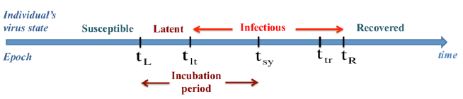
Figure 1. Ebola virus progress in an individual by using the SEIR model, where infectious occurs at $t_{L}$, latency to infectious transition at $t_{lt}$, symptoms appear at $t_{sy}$, first transmission to another susceptible at $t_{tr}$, and individual is no longer infectious (recovered) at $t_{R}$.

The transmission of the virus is then described by the following system of nonlinear ordinary differential equations:

$$\begin{cases}\dfrac{dS(t)}{dt}=-\beta S(t)I(t),\\[7.11317pt] \dfrac{dE(t)}{dt}=\beta S(t)I(t)-\gamma E(t),\\[7.11317pt] \dfrac{dI(t)}{dt}=\gamma E(t)-\mu I(t),\\[7.11317pt] \dfrac{dR(t)}{dt}=\mu I(t),\end{cases}$$ (1)

where $\beta\geq 0$ is the transmission rate; $\gamma\geq 0$ is the infectious rate; and $\mu\geq 0$ is the recovery rate. The initial conditions are given:

$$S(0)=S_{0}>0,\quad E(0)=E_{0}\geq 0,\quad I(0)=I_{0}>0,\quad R(0)=0.$$

From (1), we see that $\dfrac{d}{dt}\left[S(t)+E(t)+I(t)+R(t)\right]=0$, that is, the population $N$ is constant along time:

$$S(t)+E(t)+I(t)+R(t)=N$$

for any $t\geq 0$.

3. SEIR model with demographic effects

In the well-known basic SEIR model of Section 2, one ignores the demographic effects on the population. In this section, we study a model with vital dynamics by considering the birth and death rates. Such model is new in the Ebola context [3, 26, 27, 28, 29, 30, 38].

3.1. Model formulation

We expand the SEIR model by including demographic effects: we assume a constant birth rate $\delta$ and a natural death rate $\lambda$, obtaining

$$\begin{cases}\dfrac{dS(t)}{dt}=\delta N-\beta S(t)I(t)-\lambda S(t),\\[7.11317pt] \dfrac{dE(t)}{dt}=\beta S(t)I(t)-\gamma E(t)-\lambda E(t),\\[7.11317pt] \dfrac{dI(t)}{dt}=\gamma E(t)-\mu I(t)-\lambda I(t),\\[7.11317pt] \dfrac{dR(t)}{dt}=\mu I(t)-\lambda R(t).\end{cases}$$ (2)

Figure 2 shows the relationship between the variables of system (2), which describes the SEIR model with vital dynamics, that is, with demographic effects (birth and death).

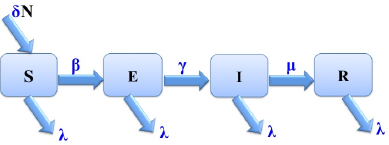
Figure 2. Compartment diagram of the SEIR model (2) with vital dynamics.

3.2. Analysis of the equilibria

Let us find the equilibria points of the system of equations (2) that describes the model. By setting the right-hand side of (2) to zero, we get

$$\delta N-\beta SI-\lambda S=0,$$ (3)

$$\beta SI-\gamma E-\lambda E=0,$$ (4)

$$\gamma E-\mu I-\lambda I=0,$$ (5)

$$\mu I-\lambda R=0.$$ (6)

By adding (3) and (4), we obtain that $\delta N-\lambda S-\left(\gamma+\lambda\right)E=0$. Then,

$$S=\dfrac{\delta N-\left(\gamma+\lambda\right)E}{\lambda}.$$ (7)

From (5) we obtain that

$$I=\dfrac{\gamma E}{\mu+\lambda}\,,$$ (8)

while from (6) it follows that

$$R=\dfrac{\mu I}{\lambda}.$$ (9)

From (4), (7) and (8), we get

$$E\left(\frac{\beta\gamma\left(\delta N-(\gamma+\lambda)E\right)}{\lambda\left(\mu+\lambda\right)}-\left(\gamma+\lambda\right)\right)=0.$$

Therefore, or $E=0$ or

$$E=\dfrac{\beta\gamma\delta N-\left(\gamma+\lambda\right)\left(\mu+\lambda\right)\lambda}{\beta\left(\gamma+\lambda\right)\gamma}.$$ (10)

For $E=0$, from (7) we obtain that $S=\dfrac{\delta N}{\lambda}$ while from (8) we get $I=0$. It follows from (9) that $R=0$. We just proved that there is a virus free equilibrium given by $P_{0}=\left(\dfrac{\delta N}{\lambda},0,0,0\right)$. From (10) we know that there is another equilibrium with

$$E^{*}=\dfrac{\delta N}{\gamma+\lambda}-\dfrac{\lambda\left(\mu+\lambda\right)}{\beta\gamma}.$$ (11)

By using $E$ given by (11) in (7), we get

$$S^{*}=\dfrac{\left(\gamma+\lambda\right)\left(\mu+\lambda\right)}{\beta\gamma},$$ (12)

by substituting (11) in (8), we obtain that

$$I^{*}=\dfrac{\gamma\delta N}{\left(\mu+\lambda\right)\left(\gamma+\lambda\right)}-\dfrac{\lambda}{\beta},$$ (13)

and finally using (11) in (9) we get

$$R^{*}=\dfrac{\mu}{\lambda}I^{*}=\dfrac{\mu}{\lambda}\left[\dfrac{\gamma\delta N}{\left(\mu+\lambda\right)\left(\gamma+\lambda\right)}-\dfrac{\lambda}{\beta}\right].$$ (14)

We just obtained the second equilibrium point $P^{*}=\left(S^{*},E^{*},I^{*},R^{*}\right)$ given by expressions (11)–(14).

Theorem 1.

Let $S(t)$, $E(t)$, $I(t)$, $R(t)$ be a solution of the SEIR model (2). Then the basic reproduction ratio is given by

$$R_{0}:=\dfrac{\beta\gamma\delta N}{\left(\mu+\lambda\right)\left(\gamma+\lambda\right)\lambda}.$$ (15)

• If $R_{0}>1$, then the equilibrium $P^{*}=\left(S^{*},E^{*},I^{*},R^{*}\right)$ of the virus is obtained, in agreement with expressions (11)–(14), and the virus is able to invade the population.

• If $R_{0}<1$, then the disease free equilibrium $P_{0}=\left(\dfrac{\delta N}{\lambda},0,0,0\right)$ of the virus is obtained, which corresponds to the case when the virus dies out (no epidemic).

Proof.

For computing the basic reproduction ratio $R_{0}$, we apply the next generation method [13, 17]. Assume that there are $n$ infective classes in the model and define the vector $\bar{x}=x_{i}$, where $x_{i}$, $i=1,2,\dots,n$, denotes the number or the proportion of individuals in the $i$th infective class. Let $F_{i}(\bar{x})$ be the rate of appearance of new infections in the $i$th class and let $V_{i}(\bar{x})=V_{i}^{-}(\bar{x})-V_{i}^{+}(\bar{x})$, where $V_{i}^{+}$ consists of transfer of individuals into class $i$ and $V_{i}^{{}^{-}}$ consists of transfer of individuals out of class $i$. The difference $F_{i}(\bar{x})-V_{i}(\bar{x})$ gives the rate of change of $x_{i}$. Notice that $F_{i}$ consists of new infections from susceptible, whereas $V_{i}$ includes the transfer of infected individuals from one infected class to another [17]. We can then form the next generation matrix from the partial derivatives of $F_{i}$ and $V_{i}$:

$$F=\left[\dfrac{\partial F_{i}(x_{0})}{\partial x_{j}}\right],\quad V=\left[\dfrac{\partial V_{i}(x_{0})}{\partial x_{j}}\right],$$

where $i,j=1,2,\dots,n$ and $x_{0}$ is the initial condition of the epidemic. The basic reproduction ratio $R_{0}$ is given by the dominant eigenvalue of the matrix $FV^{-1}$ [17]. Applying the next generation method to the SEIR model (2), and since we are only concerned with individuals that spread the infection, we only need to model the exposed, $E$, and infected, $I$, classes. Let us define the model dynamics using the equations

$$\begin{cases}\dfrac{dE(t)}{dt}=\beta S(t)I(t)-\left(\gamma+\lambda\right)E(t),\\[7.11317pt] \dfrac{dI(t)}{dt}=\gamma E(t)-\left(\mu+\lambda\right)I(t).\end{cases}$$

For this system,

$$F=\left(\begin{array}[]{cc}0&\dfrac{\beta N\delta}{\lambda}\\[7.11317pt] 0&0\end{array}\right),$$

where $\delta$ is the birth rate and $\lambda$ is the death rate, and

$$V=\left(\begin{array}[]{cc}\gamma+\lambda&0\\[7.11317pt] -\gamma&\mu+\lambda\end{array}\right).$$

Then,

$$FV^{-1}=\left(\begin{array}[]{cc}\dfrac{\beta N\delta\gamma}{\left(\gamma+\lambda\right)\left(\mu+\lambda\right)\lambda}&\dfrac{\beta N\delta}{\left(\mu+\lambda\right)\lambda}\\[9.95863pt] 0&0\end{array}\right).$$

The dominant eigenvalue $R_{0}$ of $FV^{-1}$ is given by expression (15). ∎

The recent status of the Ebola virus corresponds to the case $R_{0}>1$ [40], which we study numerically in Section 3.3.

3.3. Simulation of the SEIR model with demographic effects

Now we solve numerically the SEIR model with vital dynamics (2) by using the parameters presented in the work of Rachah and Torres [26, 29]. The early detection of Ebola virus in West Africa is characterised by $R_{0}=1.95$. Then the Ebola virus is really an epidemic, invading the populations of West Africa. The parameters $\beta=0.2$, $\gamma=0.1887$ and $\mu=0.1$, studied by Rachah and Torres [26, 29], are based on the fact that 88% of population is susceptible, 7% of population is exposed (infected but not infectious), and 5% of population is infectious. In agreement, the initial susceptible, exposed, infectious and recovered populations, are given respectively by

$$S(0)=0.88,\quad E(0)=0.07,\quad I(0)=0.05,\quad R(0)=0.$$ (16)

In the numerical resolution of the model, we take the birth rate $\delta=0.03507$ and the death rate $\lambda=0.0099$ [10, 18], with the other parameters and initial conditions as introduced by Rachah and Torres [26, 29]. The birth and death rates are obtained from the data of population of Liberia in 2014 [18].

Figure 3 shows the evolution of individuals over time. We see that the oscillations in the numbers of compartments $S$, $E$ and $I$ damp out over time, eventually reaching an equilibrium, respectively $S^{*}$, $E^{*}$ and $I^{*}$. When we calculate the value of the theoretical result (12), we find that $S^{*}=0.57$, which is equal to the $S^{*}$ computed by the numerical resolution of the model: see Figure 3a. Figure 3b shows the evolution of the exposed individuals $E(t)$ over time. Note that the equilibrium $E^{*}$ is given by (11). When we calculate the value of this theoretical result, we find $E^{*}=0.14$, which is equal to the $E^{*}$ computed by the numerical resolution of the model. Figure 3c shows the evolution of the infected individuals $I(t)$ over time. In this case the equilibrium $I^{*}$ is computed theoretically by (13), which agrees with $I^{*}=0.25$ computed by the numerical resolution of the model. Finally, Figure 3d shows the evolution of the recovered individuals $R(t)$ over time. Similarly as before, we found that the equilibrium $R^{*}=2.51$, computed theoretically by (14), coincides with the numerical resolution of the model. The fact that the reached equilibrium $(S^{*},E^{*},I^{*},R^{*})$, computed theoretically, is equal to the value found by the numerical simulation, is a validation of our study of the SEIR model with vital dynamics.

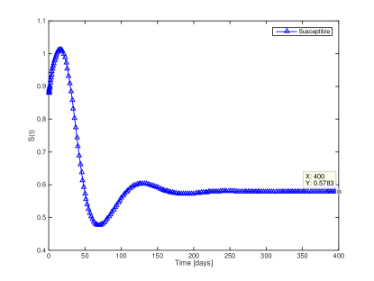
(a) Evolution of $S(t)$ with $S^{*}=0.57$

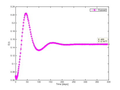
(b) Evolution of $E(t)$ with $E^{*}=0.14$

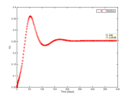
(c) Evolution of $I(t)$ with $I^{*}=0.25$

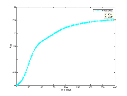
(d) Evolution of $R(t)$ with $R^{*}=2.51$

Figure 3. Evolution of individuals in compartments $S(t)$, $E(t)$, $I(t)$, $R(t)$ of the SEIR model (2) with vital dynamics, where the endemic equilibrium is given by $\left(S^{*}(t),E^{*}(t),I^{*}(t),R^{*}(t)\right)=\left(0.57,0.14,0.25,2.51\right)$.

4. Control of the virus with demographic effects through vaccination

According to recent news, a vaccine against Ebola virus is ongoing mass production, to be used in countries like Guinea, Sierra Leone and Liberia [15, 32]. Motivated by this fact, we now present a strategy for the control of the virus by introducing into the model (2) a control $u(t)$ representing the vaccination rate at time $t$. Precisely, the control $u(t)$ is the fraction of susceptible individuals being vaccinated at time $t$. Then, the mathematical model with control is given by the system of nonlinear differential equations

$$\begin{cases}\dfrac{dS(t)}{dt}=\delta N-\beta S(t)I(t)-\lambda S(t)-u(t)S(t),\\[7.11317pt] \dfrac{dE(t)}{dt}=\beta S(t)I(t)-\gamma E(t)-\lambda E(t),\\[7.11317pt] \dfrac{dI(t)}{dt}=\gamma E(t)-\mu I(t)-\lambda I(t),\\[7.11317pt] \dfrac{dR(t)}{dt}=\mu I(t)-\lambda R(t)+u(t)S(t).\end{cases}$$ (17)

The goal of the adopted strategy is to reduce the infected individuals and the cost of vaccination on a fixed time interval. Precisely, the optimal control problem consists of minimizing the objective functional $J$,

$$J(I,u)=\int_{0}^{t_{end}}\left[I(t)+\dfrac{\tau}{2}u^{2}(t)\right]dt\longrightarrow\min,$$ (18)

where $u(t)$ is the control variable, which represents the vaccination rate at time $t$, and the parameters $\tau$ and $t_{end}$ denote, respectively, the weight on the cost of vaccination and the duration, in days, of the vaccination program. In our study of the control of the virus, we use the parameters of Section 3.3 with $\tau=0.02$ and $t_{end}=90$. For the numerical solution of the optimal control problem, we have used the ACADO solver [4], which is based on a multiple shooting method, including automatic differentiation and based ultimately on the semidirect multiple shooting algorithm of Bock and Pitt [7]. The ACADO solver comes as a self-contained public domain software environment, written in C++, for automatic control and dynamic optimization [4].

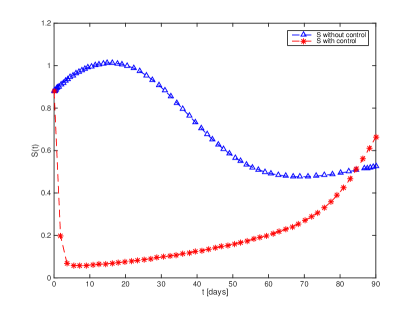
(a) Susceptible individuals $S(t)$

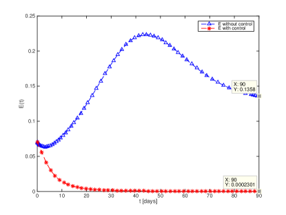
(b) Exposed individuals $E(t)$

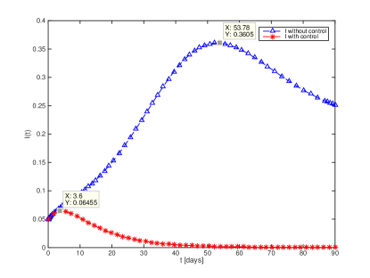
(c) Infected individuals $I(t)$

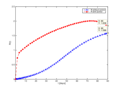
(d) Recovered individuals $R(t)$

Figure 4. Comparison between the curves of individuals $S(t)$, $E(t)$, $I(t)$, $R(t)$, in case of optimal control of (17)–(18) versus without control (2).

Figure 4 shows, respectively, the significant difference in the number of susceptible, exposed, infected and recovered individuals, with and without control, along time. As expected, the number of susceptible individuals $S(t)$ decrease rapidly in case of vaccination (see Figure 4a), beginning to increase as we decrease vaccination: compare Figure 4a of $S(t)$ with Figure 5, which represents the optimal control function $u(t)$ along time.

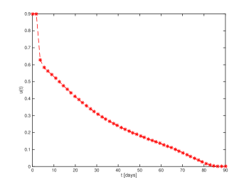
Figure 5. The optimal control function $u(t)$ for problem (17)–(18) with initial conditions (16), $t\in[0,t_{end}]$, $t_{end}=90$ days, and $\tau=0.02$.

Figure 4b shows that the number of exposed individuals decreases rapidly in case of control. In the same figure, the curve of exposed shows that the period of incubation of the virus is $22$ days in case of optimal control against more than $90$ days in the absence of any control. In Figure 4c, the time-dependent curve of infected individuals shows that the peak of the curve of infected individuals is less important in presence of control. In fact, the maximum value on the infected curve $I$ under optimal control is 0.06%, against 0.36% without any control (see Figure 4c). Figure 4d shows that the number of recovered individuals increases rapidly in presence of control. The other important effect of control, which we can see in Figure 4d, is the period of infection, which is less important in case of control of the virus. The value of the period of infection is $50$ days in case of optimal control, in contrast with more than $90$ days without vaccination. In conclusion, one can say that Figure 4 shows the effectiveness of optimal vaccination in controlling Ebola.

5. Ebola model with vital dynamics and induced death rates

In this section, we study a second Ebola model with demographic effects by increasing the death rates of the exposed and infectious classes of the model, that is, by considering induced death rates $\lambda_{E}$ and $\lambda_{I}$ associated to the exposed and infected individuals, respectively.

5.1. Model formulation

If we change the previous SEIR model (17) by increasing the death rates of the exposed and infectious classes, by adding induced death rates $\lambda_{E}$ and $\lambda_{I}$, with $\lambda_{I}>\lambda_{E}>0$, then our SEIR system becomes the one of Figure 6, where we show the relationship between the variables of the new system.

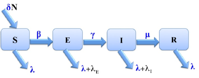
Figure 6. Compartment diagram of the SEIR model (19) with induced death rates $\lambda_{E}$ and $\lambda_{I}$ for the exposed and infectious classes, respectively.

Mathematically, the SEIR model with induced death rates is described by the following system of equations:

$$\begin{cases}\dfrac{dS(t)}{dt}=\delta N-\beta S(t)I(t)-\lambda S(t),\\[7.11317pt] \dfrac{dE(t)}{dt}=\beta S(t)I(t)-\gamma E(t)-\left(\lambda+\lambda_{E}\right)E(t),\\[7.11317pt] \dfrac{dI(t)}{dt}=\gamma E(t)-\mu I(t)-\left(\lambda+\lambda_{I}\right)I(t),\\[7.11317pt] \dfrac{dR(t)}{dt}=\mu I(t)-\lambda R(t).\end{cases}$$ (19)

Next, we study (19), which we then show to describe in a very accurate way the recent reality of Ebola in Liberia.

5.2. Analysis of the equilibria

Let us find the equilibria points of the system of equations (19). By setting the right-hand side of (19) to zero, we find that

$$\delta N-\beta SI-\lambda S=0,$$ (20)

$$\beta SI-\gamma E-\left(\lambda+\lambda_{E}\right)E=0,$$ (21)

$$\gamma E-\mu I-\left(\lambda+\lambda_{I}\right)I=0,$$ (22)

$$\mu I-\lambda R=0.$$ (23)

By adding (20) and (21), we obtain that

$$S=\dfrac{\delta N-\left(\gamma+\lambda+\lambda_{E}\right)E}{\lambda}.$$ (24)

From (22) we obtain that

$$I=\dfrac{\gamma E}{\mu+\lambda+\lambda_{I}},$$ (25)

while from (23) it follows that

$$R=\dfrac{\mu}{\lambda}I.$$ (26)

Using (24) and (25) in (21), one gets

$$E\left(\dfrac{\beta\left(\delta N-(\gamma+\lambda+\lambda_{E})E\right)\gamma}{\lambda\left(\mu+\lambda+\lambda_{I}\right)}-\left(\gamma+\lambda+\lambda_{E}\right)\right)=0,$$

that is, or $E=0$ or

$$E=\dfrac{\beta\gamma\delta N-\left(\gamma+\lambda+\lambda_{E}\right)\left(\mu+\lambda+\lambda_{I}\right)\lambda}{\beta\left(\gamma+\lambda+\lambda_{E}\right)\gamma}.$$ (27)

If $E=0$, then from (24) we obtain $S=(\delta N)/\lambda$, while from (25) $I=0$, which implies by (26) that $R=0$. Concluding, the virus free equilibrium is

$$P_{0}=\left(\dfrac{\delta N}{\lambda},0,0,0\right).$$ (28)

The endemic equilibrium $E^{*}$ is given by (27), that is,

$$E^{*}=\dfrac{\delta N}{\gamma+\lambda+\lambda_{E}}-\dfrac{\lambda\left(\mu+\lambda+\lambda_{I}\right)}{\beta\gamma}.$$ (29)

By using $E$ given by (29) in (24), we get

$$S^{*}=\dfrac{\left(\gamma+\lambda+\lambda_{E}\right)\left(\mu+\lambda+\lambda_{I}\right)}{\beta\gamma},$$ (30)

while substituting $E$ given by (29) into (25), we obtain that

$$I^{*}=\dfrac{\gamma\delta N}{\left(\mu+\lambda+\lambda_{I}\right)\left(\gamma+\lambda+\lambda_{E}\right)}-\dfrac{\lambda}{\beta}.$$ (31)

Finally, using (26), one gets

$$R^{*}=\dfrac{\mu}{\lambda}I^{*}=\dfrac{\mu}{\lambda}\left[\dfrac{\gamma\delta N}{\left(\mu+\lambda+\lambda_{I}\right)\left(\gamma+\lambda+\lambda_{E}\right)}-\dfrac{\lambda}{\beta}\right].$$ (32)

The equilibrium point is then $P^{*}=\left(S^{*},E^{*},I^{*},R^{*}\right)$ with expressions for $S^{*}$, $E^{*}$, $I^{*}$ and $R^{*}$ given by (29)–(32).

Theorem 2.

Let $S(t)$, $E(t)$, $I(t)$, $R(t)$ be a solution of the SEIR model (19). Then the basic reproduction ratio is given by

$$R_{0}:=\dfrac{\beta\gamma\delta N}{\left(\mu+\lambda+\lambda_{I}\right)\left(\gamma+\lambda+\lambda_{E}\right)\lambda}.$$ (33)

• If $R_{0}>1$, then the equilibrium $P^{*}=\left(S^{*},E^{*},I^{*},R^{*}\right)$ of the virus is obtained, in agreement with expressions (29)–(32). In this case, the virus is able to invade the population.

• If $R_{0}<1$, then the disease free equilibrium $P_{0}$ (28) is obtained. It corresponds to the case when the virus dies out (no epidemic).

Proof.

We apply the next generation method to the model (19). Here,

$$F=\left(\begin{array}[]{cc}0&\dfrac{\beta N\delta}{\lambda}\\[7.11317pt] 0&0\end{array}\right),$$

where $\delta$ is the birth rate and $\lambda$ is the death rate of susceptible, and

$$V=\left(\begin{array}[]{cc}\gamma+\lambda+\lambda_{E}&0\\[7.11317pt] -\gamma&\mu+\lambda+\lambda_{I}\end{array}\right).$$

Then, $R_{0}$ is the dominant eigenvalue of $FV^{-1}$, which is given by (33). ∎

Note that if $\lambda_{I}=\lambda_{E}=0$, then Theorem 2 reduces to Theorem 1.

5.3. SEIR model with demographic effects and induced death rates, and Liberia’s 2014 Ebola outbreak

Now, we present a modeling study of the real outbreak of Ebola virus occurred in Liberia in 2014 by using World Health Organization (WHO) data. The epidemic data used in this study is available at [41]. Let us start by the analysis of the parameters of the SEIR model with demographic effects and induced death rates. The birth rate $\delta=0.03507$ and death rate $\lambda=0.0099$ of the model are obtained from the specific statistical data of the demography of Liberia, available at [18]. To estimate the parameters $\beta$, $\gamma$, $\mu$, $\lambda_{E}$ and $\lambda_{I}$, we adapted the initialization of $I$ with the reported data of WHO by fitting the real data of confirmed cases of infectious in Liberia. The result of fitting is shown in Figure 7.

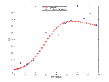
Figure 7. Graph of infected obtained from (19) and (37) versus the real data of confirmed cases for the 2014 Ebola outbreak occurred in Liberia [41].

The comparison between the curve of infectious obtained by our simulation and the reported data of confirmed cases by WHO shows that the mathematical model (19) fits well the real data by using $\beta=0.299$ as the rate of transmission, $\gamma=0.034$ as the rate of infectious, $\mu=0.0859$ as the recovery rate, and $\lambda_{E}=0.0003366$ and $\lambda_{I}=0.0031$ as induced death rates. To measure the goodness of fit, we have used a deterministic approach for the estimation of the parameters. Precisely, our fitting procedure has used a least squares method of the nonlinear system of ordinary differential equations that describes the model. According to the definition of the least squares method, the best-fit curve is the one that provides a minimal squared sum of deviation from real data. In our case, the fitting procedure is associated with the numerical resolution of the nonlinear system of ordinary differential equations (19) that describes the model. Accurately, the parameters were estimated by solving the following nonlinear programming optimization problem:

$$\begin{array}[]{ll}\mbox{minimize}&\mathcal{D}=\displaystyle\sum_{j=1}^{n}\left(I_{\text{real},j}-I_{\text{siml},j}\right)^{2}\\ \mbox{subject to}&\mbox{equations of the model}\,\eqref{SEIR_BD2},\end{array}$$ (36)

where $I_{\text{real},j}$ corresponds to real data and $I_{\text{siml},j}$ to the one obtained from the resolution of the nonlinear system of ordinary equations (19). The goodness of fit is measured by computing the value of the objective function $\mathcal{D}$ of (36), which is in our case equal to $0.0002$. By comparing the values of $\lambda_{E}$ and $\lambda_{I}$ with the value of the death rate $\lambda$, we remark that $\lambda_{E}=0.0340\lambda=3.4\%\lambda$ and $\lambda_{I}=0.3131\lambda=31.31\%\lambda$. By using the value of Liberia’s population, which is estimated at $P=4.4$ million in $2014$, and the number of confirmed infectious cases obtained from WHO, which is given by $d=230000$, we fix $I(0)=\dfrac{d}{P}$, meaning that the confirmed number of infectious cases represents $5.23\%$ of the total population. The initial susceptible, exposed, infectious and recovered populations, are given respectively by

$$S(0)=0.8977,\quad E(0)=0.05,\quad I(0)=0.0523,\quad R(0)=0.$$ (37)

Figure 7 gives the curve of infectious individuals simulated with (19) subject to (37) and the one obtained from the WHO real data. Note that the choice of $I(0)$ in (37) is in agreement with WHO’s data shown in Figure 7. The evolution of all groups of individuals, over time, is shown in Figure 8.

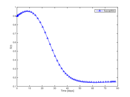
(a) Evolution of $S(t)$ with $S(0)=0.8977$

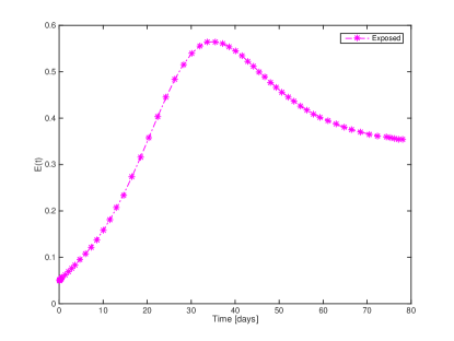
(b) Evolution of $E(t)$ with $E(0)=0.05$

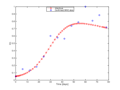
(c) Evolution of $I(t)$ with $I(0)=0.0523$

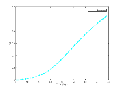
(d) Evolution of $R(t)$ with $R(0)=0$

Figure 8. Evolution of individuals in compartments $S(t)$, $E(t)$, $I(t)$ and $R(t)$ of the SEIR model (19) with vital dynamics and induced death rates, where the initial numbers of susceptible, exposed, infectious, and recovered groups and the parameter values of the model are described in Section 5.3.

6. Conclusion

We investigated several SEIR models in the context of the recent Ebola outbreak in West Africa. Our aim was to study the properties and usefulness of SEIR models with respect to Ebola. We began by presenting the basic SEIR model and its mathematical analysis. Then, we added to the model demographic effects in order to analyze the equilibria with vital dynamics. The system of equations of the model was solved numerically. The numerical simulations confirm the theoretical analysis of the equilibria of the model. Moreover, using optimal control, we controlled the propagation of the virus through vaccination, reducing the number of infected individuals and taking into account the cost of vaccination. Finally, we considered a more complete model with induced death rates and have shown its usefulness with respect to Liberia’s outbreak of 2014.

References

- [1] J. Alton. The Ebola Survival Handbook. Skyhorse Publishing, New York, 2014.
- [2] A. Atangana, E. F. Doungmo Goufo. On the mathematical analysis of Ebola hemorrhagic fever: deathly infection disease in West African countries, BioMed Research International 2014 (2014), Art. ID 261383, 7 pp.
- [3] I. Area, H. Batarfi, J. Losada, J. J. Nieto, W. Shammakh, A. Torres. On a fractional order Ebola epidemic model, Adv. Difference Equ. 2015 (2015), Art. ID 278, 12 pp.
- [4] D. Ariens, B. Houska, H. J. Ferreau. ACADO Toolkit User’s Manual, Toolkit for Automatic Control and Dynamic Optimization, 2010. http://www.acadotoolkit.org
- [5] M. Barry, F. A. Traoré, F. B. Sako, D. O. Kpamy, E. I. Bah, M. Poncin, C. Keita, M. Cisse, A. Touré. Ebola outbreak in Conakry, Guinea: Epidemiological, clinical, and outcome features. Médecine et Maladies Infectieuses 44 (2014), no. 11–12, 491–494.
- [6] J. Bartlett, J. DeVinney, E. Pudlowski. Mathematical modeling of the 2014/2015 Ebola epidemic in West Africa, SIAM Undergraduate Research Online 9 (2016), 87–102.
- [7] H. G. Bock, K. J. Pitt. A multiple shooting algorithm for direct solution of optimal control problems. Proc. 9th IFAC World Congress, Budapest, Pergamon Press, 1984, 243–247.
- [8] L. Borio et al. [Working Group on Civilian Biodefense; Corporate Author]. Hemorrhagic fever viruses as biological weapons: medical and public health management. Journal of the American Medical Association 287 (2002), no. 18, 2391–2405.
- [9] H. Boujakjian. Modeling the spread of Ebola with SEIR and optimal control, SIAM Undergraduate Research Online 9 (2016), 299–310.
- [10] F. Brauer, P. D. V. Driessche, J. Wu. Mathematical Epidemiology. Lectures Notes in Mathematics 1945, Mathematical Biosciences Subseries, 2008.
- [11] E. K. Chapnick. Ebola Myths & Facts. Wiley & Sons, 2015.
- [12] O. Diekmann, H. Heesterbeek, T. Britton. Mathematical tools for understanding infectious disease dynamics, Princeton Series in Theoretical and Computational Biology, Princeton Univ. Press, Princeton, NJ, 2013.
- [13] O. Diekmann, J. A. P. Heesterbeek, J. A. J. Metz. On the definition and the computation of the basic reproduction ratio in models for infectious diseases in heterogeneous populations. J. Math. Biol. 28 (1990), no. 4, 365–382.
- [14] S. F. Dowell, R. Mukunu, T. G. Ksiazek, A. S. Khan, P. E. Rollin, C. J. Peters. Transmission of Ebola hemorrhagic fever: a study of risk factors in family members, Kikwit, Democratic Republic of the Congo, 1995. Commission de Lutte contre les Epidémies à Kikwit. J. Infect. Dis. 179 (1999), Suppl. 1, S87–S91.
- [15] Embaixada da República Popular da China no Brasil. China terá produção em massa de vacina contra vírus Ebola, 14/Oct/2015. http://br.china-embassy.org/por/szxw/t1305911.htm
- [16] H. Gaff, E. Schaefer. Optimal control applied to vaccination and treatment strategies for various epidemiological models. Math. Biosci. Eng. 6 (2009), no. 3, 469–492.
- [17] J. M. Heffernan, R. J. Smith, L. M. Wahl. Perspectives on the basic reproductive ratio. J. R. Soc. Interface 2 (2005), 281–293.
- [18] IndexMundi. http://www.indexmundi.com.
- [19] W. O. Kermack, A. G. McKendrick. Contributions to the mathematical theory of epidemics–I. 1927. Bull Math Biol. 53 (1991), 33–55.
- [20] W. O. Kermack, A. G. McKendrick. Contributions to the mathematical theory of epidemics–II. The problem of endemicity. 1932. Bull Math Biol. 53 (1991), 57–87.
- [21] M. Kretzschmar. Ring Vaccination and Smallpox Control. Emerging Infectious Diseases 10 (2004), no. 5, 832–841.
- [22] J. Legrand, R. F. Grais, P. Y. Boelle, A. J. Valleron, A. Flahault. Understanding the dynamics of Ebola epidemics. Epidemiol. Infect. 135 (2007), no. 4, 610–621.
- [23] Jr. I. M. Longini, E. Ackerman. An optimization model for influenza A epidemics. Mathematical Biosciences 38 (1978), no. 1-2, 141–157.
- [24] D. K. Mamo, P. R. Koya. Mathematical modeling and simulation study of SEIR disease and data fitting of Ebola epidemic spreading in West Africa, Journal of Multidisciplinary Engineering Science and Technology 2 (2015), no. 1, 106–114.
- [25] C. J. Peters, J. W. LeDuc. An introduction to Ebola: the virus and the disease. Journal of Infectious Diseases 179 (1999), Suppl. 1, ix–xvi.
- [26] A. Rachah, D. F. M. Torres. Mathematical modelling, simulation and optimal control of the 2014 Ebola outbreak in West Africa. Discrete Dyn. Nat. Soc. 2015 (2015), Art. ID 842792, 9 pp. arXiv:1503.07396
- [27] A. Rachah, D. F. M. Torres. Optimal control strategies for the spread of Ebola in West Africa. J. Math. Anal. 7 (2016), no. 1, 102–114. arXiv:1512.03395
- [28] A. Rachah, D. F. M. Torres. Modeling, dynamics and optimal control of Ebola virus spread. Pure and Applied Functional Analysis 1 (2016), no. 2, 277–289. arXiv:1603.05794
- [29] A. Rachah, D. F. M. Torres. Dynamics and optimal control of Ebola transmission. Math. Comput. Sci. 10 (2016), no. 3, 331–342. arXiv:1603.03265
- [30] A. Rachah, D. F. M. Torres. Predicting and controlling the Ebola infection. Math. Methods Appl. Sci., in press. DOI:10.1002/mma.3841 arXiv:1511.06323
- [31] Report of an International Commission. Ebola haemorrhagic fever in Zaire, 1976. Bull. World Health Organ. 56 (1978), no. 2, 271–293.
- [32] Reuters. Two new trials of Ebola vaccines begin in Africa and Europe, http://voicesofafrica.co.za/two-new-trials-ebola-vaccines-begin-africa-europe
- [33] H. S. Rodrigues, M. T. T. Monteiro, D. F. M. Torres. Dynamics of dengue epidemics when using optimal control. Math. Comput. Modelling 52 (2010), no. 9-10, 1667–1673. arXiv:1006.4392
- [34] H. S. Rodrigues, M. T. T. Monteiro, D. F. M. Torres. Vaccination models and optimal control strategies to dengue. Math. Biosci. 247 (2014), no. 1, 1–12. arXiv:1310.4387
- [35] T. C. Smith. Ebola. Deadly Diseases and Epidemics, Chelsea House Publisher, 2006.
- [36] T. C. Smith. Heymann Ebola and Marburg Virus. Second Edition. Deadly diseases and epidemics, Chelsea House Publisher, 2010.
- [37] Uganda Ministry of Health. An outbreak of Ebola in Uganda. Trop. Med. Int. Health. 7 (2002), no. 12, 1068–1075.
- [38] X.-S. Wang, L. Zhong. Ebola outbreak in West Africa: real-time estimation and multiple-wave prediction. Math. Biosci. Eng. 12 (2015), no. 5, 1055–1063.
- [39] WHO, World Health Organization. Report of an International Study Team. Ebola haemorrhagic fever in Sudan 1976. Bull. World Health Organ. 56 (1978), no. 2, 247–270.
- [40] WHO, World Health Organization. Ebola Situation Reports. http://apps.who.int/ebola/ebola-situation-reports
- [41] WHO, World Health Organization. Ebola Data and Statistics. http://apps.who.int/gho/data/view.ebola-sitrep.ebola-country-LBR.