Abstract

As part of a project to better characterize comparatively bright, yet little studied cataclysmic variables time resolved photometry of the three eclipsing novalike variables EC 21178-5417, GS Pav und V345 Pav is presented. Previously known orbital periods are significantly improved and long-term ephemeris are derived. Variations of eclipse profiles, occurring on time scales of days to weeks, are analyzed. Out of eclipse the light curves are characterized by low scale flickering superposed on more gradual variations with amplitudes limited to a few tenths of a magnitude and profiles which at least in EC 21178-5417 and GS Pav roughly follow the same pattern in all observed cycles. Additionally, signs for variations on the time scale of some tens of minutes are seen in GS Pav, most clearly in two subsequent nights when in the first of these a signal with a period of 15.7 min was observed over several hours. In the second night variations with twice this period were seen. While no additional insight could be gained on quasi periodic oscillations (QPOs) and dwarf nova oscillations in EC 21178-5417, previously detected by Warner et al. (2003), and while such oscillations could not be found in V345 Pav, stacked power spectra of GS Pav clearly reveal the presence of QPOs over time intervals of several hours with periods varying between 200 sec and 500 sec in that system.

.

Keywords: Stars: binaries: close – Stars: novae, cataclysmic variables – Stars: individual: EC 21178-5417 – Stars: individual: GS Pav – Stars: individual: V345 Pav

1 Introduction

Cataclysmic variables (CVs) are interactive binaries where a late type, low mass star which is normally on or close to the main sequence transfers matter to a white dwarf. The number of known systems of this kind has grown enormously in recent years mainly due to numerous detections of CVs in large scale surveys. However, most of these newly detected systems are rather faint in their normal brightness state. Therefore, the characterization of their individual properties is expensive because is requires large telescopes.

On the other hand, it is much easier to perform detailed studies of the brighter CVs, most of which are known for a long time. It is therefore surprising that even among these stars an appreciable number has not yet been adequately characterized to be certain about basic parameters. In some cases even the very class membership is not confirmed.

I therefore started a small observing program aimed at a better understanding of these so far neglected stars and to fill in evident gaps in our knowledge about them. For this purpose I selected a number of little studied southern CVs and suspected CVs bright enough to be easily observed with comparatively small telescopes. The emphasize of this program lies on photometry with a high time resolution aimed at the detection and characterization of short and medium time scale variations such as flickering and orbital variability.

Here, I present a photometric study of three eclipsing novalike variables, namely EC 21178-5417, GS Pav and V345 Pav in order to derive improved orbital ephemeris and to characterize in some detail the light curves in and out of eclipse. In Sect. 2 the observations and data reduction techniques are described. In Sects. 3 – 5 the results for the individual target stars are presented. In each case, eclipse timings are measured and ephemeris are calculated, the eclipse profiles are studied and the out-of-eclipse variations on various time scales are analyzed. Finally, a short summary in Sect. 6 concludes this paper.

2 Observations and data reductions

The target stars were observed with the 0.6-m Zeiss and 0.6-m Boller & Chivens telescopes of the Observatório do Pico dos Dias (OPD), operated by the Laboratório Nacional de Astrofísica, Brazil. During various observing missions, each lasting a couple of nights, time series imaging of the field around the target stars was performed using cameras of type Andor iXon EMCCD DU-888E-C00-#BV equipped with back illuminated, visually optimized CCDs. In order to resolve the expected rapid flickering variations the integration times were kept short. Together with the small readout times of the detectors this resulted in a time resolution of the order of 5 sec. In order to maximize the count rates in these short exposure intervals no filters were used (i.e., the observations were taken in integral “white” light). Therefore, it was not possible to calibrate the stellar magnitudes. Instead, the brightness is expressed as the magnitude difference between the target and a nearby comparison star. This is not a severe limitation in view of the purpose to the observations. However, even so the differential magnitudes can be roughly transformed into $V$, considering that the white light passband has an effective wavelength close to that of the $V$ band (Bruch 2017). To do so requires knowledge of the brightness of the comparison stars. The average of their magnitudes, taken from the SPM4 (Girard et al. 2011), Nomad (Zacharias et al. 2005) and UCAC4 (Zacharias et al. 2013) catalogues is: $V=12.40\pm 0.06$ (EC 21178-5417), $V=14.38\pm 0.19$ (GS Pav) and $V=12.14\pm 0.17$ (V345 Pav).

During the various missions different CCDs had to be used. It must be expected that their characteristics are not identical. Although the differences should not be drastic because the CCDs were all of the same type, I find significantly varying magnitude differences between the comparison stars and several check stars between missions, while during a given mission they remained virtually constant. This behaviour may be attributed to slight differences of the wavelenth dependent detector sensitivity, enhanced by the broad white light passband. Therefore, the differential magnitudes between the target stars and the comparison stars may be compared within a given observing run, but any differences between missions are not reliable. This holds true for EC 21178-5417 and V345 Pav but not for GS Pav in which case the magnitude differences between comparison and check stars remained quite stable.

A summary of the photometric observations is given in Table 1.

Table 1: Journal of photometric observations

Name	Obs. Date	Start	End	Time	Number
		(UT)	(UT)	Res. (s)	of Integr.
EC 21178-5417	2015 Jul 14	23:04	29:02	15.5	3 922
	2015 Aug 10/11	23:21	27:23	15.5	4 961
	2015 Aug 12	23:00	27:10	16.5	3 000
	2015 Aug 13	22:40	26:48	16.5	3 000
	2015 Aug 14	22:49	26:57	16.5	2 999
	2015 Aug 15	22:47	26:50	16.5	2 125
	2016 May 10	26:57	27:00	15.5	2 660
	2016 May 12	25:51	28:08	15.5	1 531
GS Pav	2004 Aug 16/17*	22:52	21:49	15 – 20	2 474
	2016 Jun 09	25:59	28:22	15.5	2 100
	2016 Jun 28	23:05	28:54	15.5	3 989
	2016 Jun 29	21:31	22:46	15.5	2 406
	2016 Aug 08/09	22:58	24:35	15.5	3 227
	2016 Aug 11	21:15	25:26	15.5	3 000
	2016 Aug 12	20:46	25:36	15.5	3 495
	2016 Sep 06	21:48	23:40	15.5	1 346
	2016 Sep 06/07	22:21	23:18	15.5	1 863
V345 Pav	2015 May 22	25:36	27:13	16.5	1 993
	2015 Jun 09	22:36	27:32	16.5	2 998
	2015 Jun 10	21:58	25:13	16.5	2 000
	2015 Jun 11	21:50	25:30	16.5	1 997
	2015 Jun 12	21:49	25:04	16.5	2 000
	2015 Aug 10	21:36	22:59	15.5	1 000
	2015 Aug 11/12	21:24	22:39	15.5	3 495
	2015 Aug 12/13	21:28	22:29	15.5	3 596
	2015 Aug 13/14	21:27	22:30	15.5	3 494
	2015 Aug 14/15	21:57	22:37	15.5	3 303
	2016 Jun 09	24:09	25:50	15.5	1 158
	2016 Jun 10	24:03	25:25	15.5	1 000
*archival data, filter $B$ (unpublished)

Basic data reductions (biasing, flat-fielding) was performed using IRAF. For the construction of light curves aperture photometry routines implemented in the MIRA software system (Bruch 1993) were employed. The same system was used for all further data reductions and calculations. All timing information was transformed into barycentric Julian Dates on the barycentric dynamical time scale (BJD-TDB), following Eastman et al. (2010). Examples of the light curves are shown in Fig. 1.

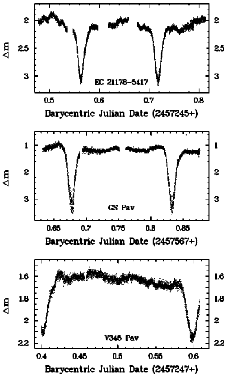
Figure 1: Light curves of EC 21178-5417 (top), GS Pav (centre) and V345 Pav (bottom) as examples of typical orbital light curves of these systems.

3 EC 21178-5417

Not much is known about EC 21178-5417. Identified as a blue object in the Edinburgh Cape survey (Stobie et al. 1997), it was first mentioned as a cataclysmic variable by Warner et al. (2003) who found it to be an eclipsing novalike system and quote an orbital period of 3.708 h. Since that paper was exclusively concerned with dwarf nova oscillations (DNOs) and quasi-periodic oscillations (QPOs) in a larger sample of CVs, Warner et al. (2003) did not investigate further properties of EC 21178-5417 apart from that particular aspect. They postponed details about the light curve and the spectrum to another paper which, however, never appeared.

3.1 Eclipse timings and ephemeris

The light curves contain a total of 10 eclipses. The minimum times were determined by the time of minimum $t_{\rm m}$ of a Gaussian and a polynomial fit to the data within a range of $\pm$10 min around the minimum. Changing the degree of the polynomial has only a minute influence of the results. In particular, there are no systematic variations with the polynomial degree. Choosing all values between 2 and 9 and adding the minimum of the fitted Gaussian resulted in an average standard deviation of 10.8 sec for $t_{\rm m}$ of the 10 eclipses. Thus, this value may be regarded as the typical error of the eclipse time determination.

I adopted the average values of $t_{\rm m}$ for the different polynomial degrees and the Gaussian as the time of minimum of eclipses. They are listed in Tab. 2 where eclipse no. #0 is arbitrarily assigned to the first eclipse observed on 2015, August 11.

Table 2: Eclipse epochs

EC 21178-5417			GS Pav			V345 Pav
Ecl. No.	BJD-TDB	$O-C$	Ecl. No.	BJD-TDB	$O-C$	Ecl. No.	BJD-TDB	$O-C$
	(2400000+)	(sec)		(2400000+)	(sec)		(2400000+)	(sec)
-180	57217.74883	31.0	-53662	49235.73769	-35.7	-47429	47769.28105	24.8
0	57245.56294	-42.9	-53650	49237.60208	64.6	-47428	47769.47865	-18.1
1	57245.71788	-7.3	-53644	49238.53368	62.8	-47419	47771.26145	-23.9
7	57246.64511	-1.7	-53643	49238.68828	4.9	-47418	47771.45985	2.3
8	57246.79950	-13.8	-50035	49798.90168	-36.7	-47414	47772.25245	20.8
14	57247.72708	22.4	-50029	49799.83468	82.6	-47287	47795.42915	-29.1
20	57248.65353	-39.9	-49502	49881.66098	0.4	-47287	47797.41065	17.3
27	57249.73531	-32.5	-49501	49881.81538	-74.7	0	57164.79457	20.6
1768	57518.76817	-3.1	-49321	49909.76478	-4.4	90	57182.62304	3.1
1781	57520.77724	15.3	-49320	49909.91978	-27.8	95	57183.61366	14.8
			-49231	49923.73828	-73.0	100	57184.60394	-2.5
			-49089	49945.78638	-92.8	105	57185.59431	-12.7
			-48896	49975.75488	28.5	407	57245.41978	18.8
			-48871	49979.63688	50.3	412	57246.41023	16.1
			-27908	53234.56104	116.0	413	57246.60815	0.9
			-116	57549.82129	-10.4	417	57247.40095	36.7
			-1	57567.67787	36.1	418	57247.59809	-46.4
			0	57567.83294	18.6	423	57248.58944	28.8
			5	57568.60883	-21.2	428	57249.57976	14.9
			269	57609.60029	-3.5	1938	57548.70474	-33.5
			282	57611.61918	26.0	1943	57549.69514	-41.2
			288	57612.55037	-8.4
			289	57612.70612	33.2

A linear least squares fit to the eclipse epochs in Tab. 2, weighted by the inverse of the error of the individual timings, yields the ephemeris

$${\rm BJD_{min}} = 2457245.56348\ (10)$$

$$+0.15452758\ (14)\times E$$

where $E$ is the cycle number. The errors are given in units of the last decimal digits. They are formal errors of the least squares fit which may sub estimate the real errors. The rms of the residuals between the observed eclipse times and those calculated from the above ephemeris (i.e., the $O-C$ values) is 25.7 sec. The $O-C$ values for the individual eclipses are included in Table 2.

3.2 Eclipse profile

Fig. 2 shows the eclipse profiles of EC 21178-5417 as a function of orbital phase. The upper (green) graph refers to the 2015, July 14, while the others show the average of all 2015, August (red) and 2016, May (blue) light curves. The latter has been shifted downward by $0^{\raisebox{0.90417pt}{\scriptsize m}}_{\raisebox{1.80835pt}{\hskip 1.18999pt.}}2$ for clarity. In all cases the data were binned in intervals of width 0.001 in phase. The average of the standard deviations of the individual magnitudes in each interval is shown as a typical error bar at the right margin just below or above the light curves. It is larger in 2015, August in spite of the less noisy average profile as compared to that of 2015, July 14 because of slight systematic differences between the seven contributing eclipses. The same is true for 2016, May, where additionally parts of the light curves (but fortunately not the eclipse bottom) were affected by passing clouds, increasing the noise.

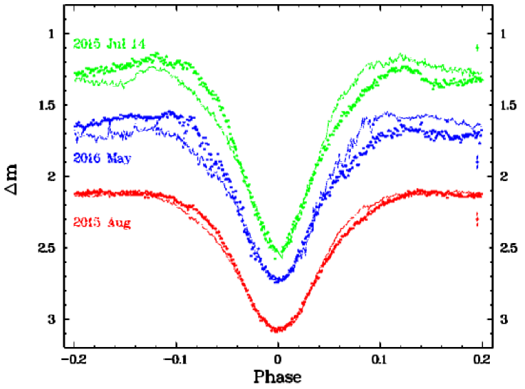
Figure 2: Eclipse profile of EC 21178-5417 on 2015, July 14 (green) and average profile of seven (red) and two (blue) eclipses observed in 2015, August and 2016, May, respectively. All light curves were binned in phase intervals of width 0.001. Error bars are indicated at the right margin above or below the curves. The thin continuous curves are the eclipse profiles mirrored at phase 0 in order to emphasize asymmetries in their upper part. (For visualization of the colours used in this figure, the reader is referred to the web version of this article.)

While the lower part of the eclipse profiles is symmetrical to a high degree, slight deviations from symmetry occur during the initial and final parts, respectively, of ingress and egress. This is more obvious when regarding the thin continuous curves in Fig. 2 which are the eclipse profiles after being mirrored at phase 0. The first part of the ingress is slightly steeper than the last part of the egress. This effect is seen (often much stronger than in the present case) in many other eclipsing cataclysmic variables and is generally attributed to different aspects of the mass transfer stream impact region on the accretion disk at the start and end of eclipse.

In order to estimate the eclipse depth the magnitude difference $\Delta m_{\rm ecl}$ between the eclipse bottom (defined as the minimum of a high degree polynomial fit to the phase interval –0.04 …0.04) and the mean magnitude $\Delta m$ in the phase intervals –0.20 …–0.18 and 0.18 …0.20, respectively, was calculated. The results are listed in Table 3. It is seen that the depth remains fairly constant at a given epoch but differs significantly on longer time scales. In particular, the eclipses were shallower during 2015, August than in 2015, July.

Table 3: Eclipse depth

EC 21178-5417		GS Pav		V345 Pav
Ecl.	depth	Ecl.	depth	Ecl.	depth
No.	(mag)	No.	(mag)	No.	(mag)
-180	1.22	-27908	3.85*	0	0.76
0	0.92	-129	2.23*	90	0.75
1	0.97	-1	2.19*	95	0.74
7	0.93	0	2.08*	100	0.75
8	0.96	5	2.39:	105	0.74
14	0.99	269	2.00*	407	0.42
20	0.93	282	2.28*	412	0.44
27	0.93	288	2.28*	413	0.50
1768	1.10	289	2.09*	417	0.43
1781	1.01	455	$>$1.79*	418	0.51
				423	0.47
				428	0.51
				1938	0.72
				1943	0.79
*$B$ band

3.3 Out-of-eclipses variations

As observed in all CVs, the out-of-eclipse variations exhibit flickering which in the present case is limited to amplitudes up to about $0^{\raisebox{0.90417pt}{\scriptsize m}}_{\raisebox{1.80835pt}{\hskip 1.18999pt.}}1$. This is on the low side of the amplitude distribution in CVs, but not unusual for systems with accretion disks in a bright state such as novalike variables and old novae (Beckemper 1995). Most of the higher frequency flickering variations are drowned in the data noise. Therefore, I refrain from a more thorough quantitative analysis.

Superposed on the flickering are variations on longer time scales. In order to study their dependency on orbital phase, the eclipses were first removed. Thereafter, the combined 2015, August and the single 2015, July light curves (the latter encompassing about 1.6 cycles) where folded on the orbital period. The results are shown in Fig. 3. The difference of the average magnitude of EC 21178-5417 outside eclipse during the two epochs is significantly larger than can be explained as being due to the use of different detectors during the respective observing missions (see Sect. 2). Therefore, it is safe to say that the star was really brighter in July than in August, although I cannot quantify by how much.

During August (lower frame), the light curve is characterized by a gradual and linear increase of brightness between phases $\phi=0.25$ and $\phi=0.65$ and then a more rapid decline until $\phi=0.8$. The disturbance seen at $0.3\leq\phi\leq 0.4$ occurs only in 2 of six cycles with data covering this phase range. The eclipses may hide a secondary maximum at $-0.2\leq\phi\leq 0.25$. This is better seen in the light curve of July 14 (upper frame) which also shows the primary maximum, now shifted to earlier phases. The approximate constancy of the profile of these variations suggest the presence of structures in the accretion disk which remain stable at least on the time scale of weeks.

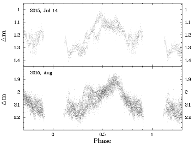
Figure 3: Phase folded out-of-eclipse light curves of EC 21178-0517 of 2015, July 14 (top) and August 11 – 15 (bottom).

I investigated the possible presence of consistent brightness variations with periods others than the orbital period $P_{\rm orb}$. For this purpose the combined 2015, August light curves (masking the eclipses) were subjected to various period search algorithms [Lomb-Scargle periodogram, Lomb (1976), Scargle (1982); power spectra following Deeming (1975); phase dispersion minimization (PDM), Stellingwerf (1978); analysis of variance (AoV), Schwarzenberg-Czerny (1989)]. To no avail: Only $P_{\rm orb}$ and its harmonics as well as their aliases caused by the window function were recovered. Pre-whitening the data, subtracting the orbital variations before the period analysis did not change the picture. Therefore, I am confident that EC 21178-5417 does not exhibit periodic variations different from $P_{\rm orb}$ which remain coherent over the several nights spanned by an observing mission.

3.4 DNOs and QPOs

Warner et al. (2003) identified EC 21178-5417 as a rich source of short period oscillations. They present an extensive list of DNOs, longer period dwarf nova oscillations (lpDNOs) and QPOs which appear for some time in the light curves observed by them and are absent at other times. The DNOs have periods between 22 sec and 26 sec (sometimes their first overtone is observed; they may also split up into more than one closely spaced components). The periods of the lpDNO (which more often than not appear simultaneously with the DNOs) range between $\sim$80 sec and $\sim$100 sec while the QPOs span a wider range between $\sim$200 sec and $\sim$500 sec. In his review on rapid oscillations in cataclysmic variables Warner (2004) discusses the relationship between DNOs, lpDNOs and QPOs in EC 21178-5417 and in other systems.

Comparing Fig. 14 of Warner et al. (2003) with the present data it is obvious that the S/N ratio of their light curves is higher. Therefore, it will be more difficult here to detect short period oscillations which may be present. Nevertheless, an effort to do so and eventually put constraints on their amplitudes is worthwhile.

When it comes to QPOs, their low coherence and often short duration (limited frequently to only a few cycles) in the presence of the ubiquitous flickering in cataclysmic variables severely hampers their detection using tools such as Fourier transforms. As Bruch (2014) pointed out, it is not obvious where to draw the borderline between QPOs and flickering. In view of these difficulties, Warner (2004) wisely (citing) “accepts only the QPOs in the light curves that are obvious to the eye”. Adopting this criterion I cannot confidently identify any QPOs in the present light curves.

DNOs (and lpDNOs) are more coherent over the time scale of hours [Warner (2004) cites $10^{3}<|dP/dt|^{-1}<10^{7}$] and are thus more easily detected in power spectra. However, since in many cases they are only present during a part of an observed light curve, they may not reveal themselves in power spectra of the entire curve. Therefore, I calculated stacked power spectra of all light curves, following Bruch (2014): Lomb-Scargle periodograms for sections of a data train, 1000 sec long, were constructed, allowing for an overlap of 900 sec between subsequent sections. The individual power spectra were then stacked on top of each other, resulting in a two dimensional representation (frequency vs. time). As an example, Fig. 4 shows the light curve of 2015, August 12 (lower left) and the corresponding stacked power spectrum (lower right). Power is coded as shown by the colour bar (upper right) where also false alarm probabilities $P_{\rm fa}=0.1$ and $P_{\rm fa}=0.01$ for peaks in the power spectra are indicated. They were calculated using Eq. 18 of Scargle (1982), the number of independent frequencies having been determined as detailed by Bruch (2016). Spectra within a time scale of 1000 sec are not independent (therefore, the length of the sections from which the power spectra are calculated, will henceforth be termed “independence limit”). Thus, only structures with a vertical extension of $>$1000 sec (the length of the double arrow at the upper left of the stacked power spectra) indicate persistent signals.

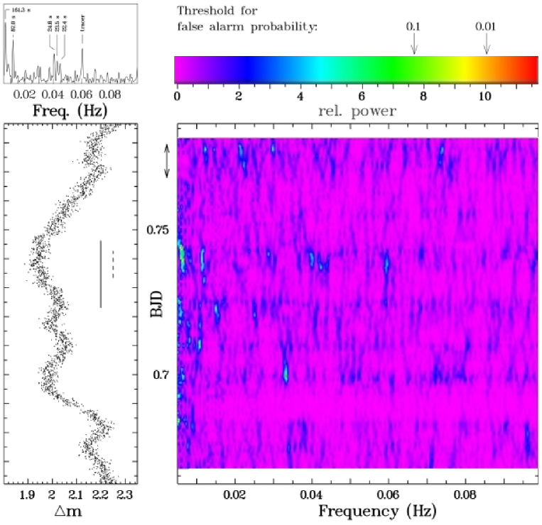
Figure 4: Out-of-eclipse light curve of EC 21178-5417 of 2015, Aug. 12 (lower left frame) and stacked power spectra of the same data (right). Spectral features within a range of 1000 sec are not independent from each other. The length of this range is indicated by a double arrow at the upper left margin of the stacked power spectra. The levels of false alarm probabilities 0.1 and 0.01 are indicated on the colour bar (upper right). The solid bar underneath the light curve indicates a section where a tracer signal of 0.06 Hz was added. The dashed line indicates a range in time where DNOs and lpDNOs may be present. An alternative representation of the power spectrum of this range is shown in the upper left frame. (For visualization of the colours used in this figure, the reader is referred to the web version of this article.)

In order to assess the sensitivity of the power spectra to oscillations, a sine wave with an amplitude of $0^{\raisebox{0.90417pt}{\scriptsize m}}_{\raisebox{1.80835pt}{\hskip 1.18999pt.}}005$ and a frequency of 0.06 Hz was added as a tracer signal to the part of the light curve marked by the solid vertical line in the lower left frame of Fig. 4. It can be identified in the stacked power spectra, but is not a particularly outstanding feature. Thus, in order to confidently identify any real oscillations in the data they should have amplitudes larger than the tracer signal. This is more than the oscillation amplitudes observed by Warner et al. (2003).

Therefore, it is not surprising that I cannot detect strong evidence for the presence of significant oscillations. The DNOs observed by Warner et al. (2003) have a frequency predominantly just above 0.04 Hz. While during some time intervals signals are seen at these frequencies, by no means they stand out against many other signals at other time intervals and frequencies. Drawing on the pre-information about the expected frequencies and the often simultaneous presence of DNOs and lpDNOs, the strongest evidence for the presence of oscillations occurs in the small time interval marked by the broken vertical line in the lower left frame of Fig. 4. An alternative representation of the power spectrum of this region is shown in the upper left frame of the figure. Three peaks corresponding to periods of 22.4 sec, 23.5 sec and 24.8 sec may represent DNOs split up into multiple components, while the peak corresponding to 87.0 sec may be a lpDNO. Additionally, a low frequency signal (161.3 sec) is the only feature in the stacked power spectrum which attains a false alarm probability below 0.01 ($P_{\rm fa}=0.002$). Thus, while oscillations such as those observed by Warner et al. (2003) may be present in our data, they cannot be considered independent detections.

The stacked power spectra of the other light curves are similar to that of 2015, August 12. In only one case, during a short period of time on 2015, August 14, possibly real signals (however, only with marginal significance) were detected simultaneously at 10.6 sec and at 161.3 sec. The former may be the overtone of a DNO at 21.2 sec, while the latter has a period identical to the low frequency oscillation observed on 2015, Aug. 12.

4 GS Pav

GS Pav was discovered as a variable star by Hoffmeister (1963). Zwitter & Munari (1995) published a spectrum. Only the Balmer emission lines can reliably be identified upon a blue continuum. Groot et al. (1998) presented the only more detailed study of GS Pav. Their photometric measurements reveiled the star to be deeply eclipsing with a period of 3.72 h. They estimated masses of the components, restricted the orbital inclination to $74^{\raisebox{0.90417pt}{\scriptsize o}}<i<83^{\raisebox{0.90417pt}{\scriptsize o}}$ and argued that the disk radius is variable which leads to a correlation between the eclipse depth and the out-of-eclipse magnitude. They also classified the system to be a novalike variable of the RW Tri subclass.

GS Pav was initially included in the present study because the observation of additional eclipses and the time difference to the observations of Groot et al. (1998) should permit to improve the precision of the orbital period by an order of magnitude. The observations listed in Tab. 1, performed within an interval of about two months, were supplemented by archival data retrieved from the LNA data bank, consisting of a light curve observed at the 1.6 m Perkin Elmer telescope of OPD on 2004, August 16. These data were obtained with a $B$ filter and span a time interval of about 3 h at a time resolution of 15 sec (first hour) and 20 sec (last two hours).

Ritter & Kolb (2003) classified GS Pav as being of the VY Scl subtype, i.e., a novalike variable which occasionally drops into a low state. Although Groot et al. (1998) found the out-of-eclipse magnitude of the star to vary, they argued that GS Pav should not be considered a VY Scl star. This is corroborated by the AAVSO long term light curve shown in Fig. 5 which shows that the star has a normal visual magnitude of $\sim$$15^{\raisebox{0.90417pt}{\scriptsize m}}$ with a limited scatter to higher and lower values. The coverage is dense enough such that substantial low states cannot hide within the gaps. Therefore, there appears to be no reason to suspect a VZ Scl nature for GS Pav.

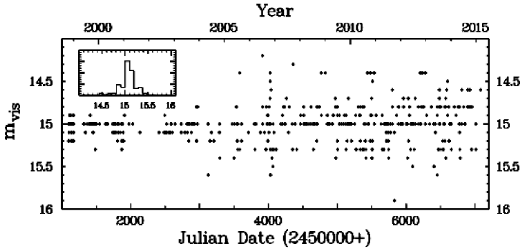
Figure 5: Long term visual light curve of GS Pav based on AAVSO data. The insert shows a histogram of the magnitude values.

4.1 Eclipse timings and ephemeris

The light curves contain a total of 9 eclipses. In order to determine the minimum epochs a range in time of approximately 14 min before and 11 min after eclipse minimum was regarded. This range encompasses the entire ingress, but avoids the shallower part at the end of egress. Restricting this exercise to a smaller range around the bottom of the eclipse is not warranted because at least in some light curves these phases are quite noisy due to the faintness of the system during mid-eclipse. The minimum times were then determined in the same way as for EC 21178-5417. Their typical error was found to be 19.0 sec. The average timings are listed in Tab. 2 together with the eclipse times measured by Groot et al. (1998). Since the latter are given in HJD expressed on the UTC time scale (P. Groot, private communication) they have been transformed into BJD-TDB, using the online tool of Eastman et al. (2010). Eclipse no. #0 is arbitrarily assigned to the second eclipse observed on 2016, June 28, noting that the ephemeris of Groot et al. (1998) are sufficiently accurate to ensure cycle count continuity to the present epoch (large negative eclipse numbers). Eclipse number -27908 refers to the archival light curve of 2004, August 16/17. Assigning weights in proportion to the inverse of the individual timing errors to the 2016 data points and the average of these weights to the data points of Groot et al. (1998), a linear least squares fit to the eclipse epochs yields the ephemeris

$${\rm BJD_{min}} = 2457567.83273\ (13)$$

$$+0.1552699235\ (36)\times E$$

The rms of the $O-C$ values is 50.6 sec in this case and the respective values for the individual eclipses are listed in Table 2.

The distribution of eclipse timings consists of two groups of data points separated by about 22 years, plus a single epoch about halfway between them. If the period of GS Pav had a significant derivative, the assumption of linear ephemeries should result in a large $O-C$ value for that point. At 116 sec it is slightly more than two times the overall rms. Thus, any period derivative of GS Pav must be so small that is has at most a marginal effect over the total time base of the present observations.

4.2 Eclipse profile

The individual eclipses of GS Pav, binned in phase intervals of width 0.005, are plotted in Fig. 6. With the exception of the uppermost curve, which represents the average profile after applying a magnitude correction to the individual light curves (defined by the average magnitude in the phase intervals –0.20 …–0.18 and 0.18 …0.20) in order to take into account night-to-night variations of the mean system brightness, all data have been left on their original differential magnitude scale (i.e., without applying vertical shifts). It is thus seen that the magnitude level just before eclipse varies within a range of $1^{\raisebox{0.90417pt}{\scriptsize m}}_{\raisebox{1.80835pt}{\hskip 1.18999pt.}}2$. Changes of several tenths of a magnitude can occur from night to night (e.g., between 2016, Aug. 11 and 12). The average eclipse profile is symmetrical around phase 0 to a high degree. This is emphasized by the broken back curve which is a mirrored version of the original profile. It only deviates from the original at the extremes of the profile due to a delayed late egress of the accretion disks. As in the case of EC 21178-5417 this suggest a phase dependent contributions of the stream impact region to the total light.

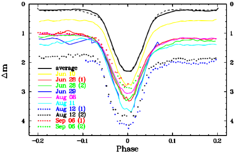
Figure 6: Eclipse profiles of GS Pav after binning the original data points in intervals of width 0.005 in phase. The solid black curve represents the average profile after applying a magnitude correction to the individual light curves (defined by the average magnitude in the phase intervals –0.20 …–0.18 and 0.18 …0.20) in order to take into account night-to-night variations of the mean system brightness. The broken back curve is a mirrored version of the average profile in order to visualize any asymmetries. (For visualization of the colours used in this figure, the reader is referred to the web version of this article.)

The eclipses of GS Pav are much deeper than in the other objects of this study. The depth $\Delta m_{\rm ecl}$ was measured in the same way as in EC 21178-5417. It is listed in Table 3.

For completeness I also measured the eclipse depth in the archival $B$ band light curve of 2004, Aug. 16/17 and include the result in Table 3. Not surprisingly for a blue object such as a CV it is significantly deeper than in the white light data.

The latter correspond roughly to the $V$ band [Bruch17]. Thus, $\Delta m\approx\Delta V$ and $\Delta m_{\rm ecl}\approx\Delta V_{\rm ecl}$ . Since the data of Groot et al. (1998) also refer to the $V$ band, a comparison with their eclipse depth measurements can be made. They find a complex correlation between $\Delta V_{\rm ecl}$ and $V$ (their Fig. 2). As was pointed out in Sect. 2, in contrast to the other two stars of this study the zero point of the differential magnitude scale for GS Pav did no change between missions. It is therefore possible to look for a similar correlation in the present data. It does not exist. A formal linear least squares fit yields a correlation coefficient of only 0.15 between these quantities and the gradient $\Delta V_{\rm ecl}/\Delta V$ has a formal error which is more than twice its nominal value.

The present observations encompass a more restricted range of both, $\Delta V_{\rm ecl}$ and $V$ than those of Groot et al. (1998). Considering the magnitude of the comparison star to GS Pav (UCAC4 102-102986) of $V=14.24$ (taken from the NOMAD catalogue; Zacharias et al. 2005) or $V=14.51$ (SPM4 catalogue; Girard et al. 2011), $\Delta m$ then translates into a $V$ magnitude of GS Pav which ranges between $14^{\raisebox{0.90417pt}{\scriptsize m}}_{\raisebox{1.80835pt}{\hskip 1.18999pt.}}8$ and $15^{\raisebox{0.90417pt}{\scriptsize m}}_{\raisebox{1.80835pt}{\hskip 1.18999pt.}}5$, while $\Delta V_{\rm ecl}$ is restricted to $1^{\raisebox{0.90417pt}{\scriptsize m}}_{\raisebox{1.80835pt}{\hskip 1.18999pt.}}8$ – $2^{\raisebox{0.90417pt}{\scriptsize m}}_{\raisebox{1.80835pt}{\hskip 1.18999pt.}}3$ (see Table 3). This corresponds to what Groot et al. (1998) call the “shallow branch”, where the eclipse depth decreases with decreasing out of eclipse brightness. In the context of their entire $\Delta V_{\rm ecl}$ – $V$ diagram they interpret the shallow branch as a range where an increase of the accretion disk radius conspires with a partial self-occultation of a flared disk to decrease $V$ while $\Delta V_{\rm ecl}$ also decreases. Here, no clear indication of such an effect is seen. Possibly, the conspiration between disk radius variations and self-occultation (disk flaring may be a function of azimuth in a time dependent manner) did not lead to a clear dependence of $\Delta V_{\rm ecl}$ on $V$ in 2016.

4.3 Out-of-eclipses variations

Flickering in GS Pav appears to occur on a similar amplitude scale as in EC 21178-5417. However, since GS Pav is significantly fainter than EC 21178-5417 (which has $V=13.65$ according to Zacharias et al. 2013) data noise makes it even more difficult to quantitatively investigate flickering here and I refrain to do so.

Most of the light curves exhibit a more or less consistent pattern of out-of-eclipse variablity as a function of orbital phase. This can be seen in Fig. 7 where all light curves with a suitable phase coverage are shown folded on the orbital period (on their original differential magnitude scale in order to preserve the long term variations of the system brightness). In order to better visualize the phase dependent variations and to reduce the noise the light curves have been binned in intervals of width 0.005.

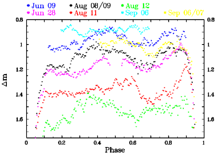
Figure 7: Phase folded out-of-eclipse light curves of GS Pav (binned in intervals of width 0.005) on the original differential magnitude scale [except for the data of 2016, August 12 (green dots) which have been shifted upwards by $0^{\raisebox{0.90417pt}{\scriptsize m}}_{\raisebox{1.80835pt}{\hskip 1.18999pt.}}3$]. (For visualization of the colours used in this figure, the reader is referred to the web version of this article.)

All light curves which cover the respective phase exhibit an increase in brightness just before eclipse ingress. This is the usual manifestation of a hot spot at the location of impact of the stream of transferred matter onto the accretion disk, as seen in numerous CVs with high orbital inclination. Apart from this, a second hump is seen, the phase of which is not constant. Its maximum occurs roughly between phase 0.3 and 0.6. The amplitude is comparable to that of the hot spot hump. This feature is only missing in the light curve obtained on 2016, September 6 (uppermost curve in Fig. 7) when the system was in a particularly bright state. As in EC 21178-5417 the persistent phase dependent variations point at azimuthal structures in the accretion disk.

In order to investigate the presence of other than these obvious periodicities I combined light curves observed close in time (set #1: June 9 and 10; set #2: August 8/9, 11 and 12; set #3: September 6 and 6/7) after removal of the eclipses and subtraction of the average nightly differential magnitude in order to remove night-to-night variations. Lomb-Scargle periodograms where then calculated. As expected in view of the phase folded light curves of Fig. 7, they are dominated by strong signals at twice the orbital frequency and its aliases. However, a different picture emerges after removal of variations on longer times scales ($>$0.05 days). This was achieved by applying a Fourier filter to the light curves which removes variations more rapid than this, and subsequent subtraction of the filtered version from the original light curve.

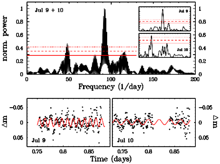
Figure 8: Top: Power spectrum of the combined light curves of GS Pav on 2016, June 9 and 10 after removing variations on time scales above 0.05 days and binning in intervals of $\approx$43 sec (0.0005 days). The inserts contain the powerspectra of the light curves of the individual nights. The red solid, dashed and dotted horizontal lines indicate the power level for false alarm probabilities of 0.01, 0.001 and 0.0001, respectively. Bottom: The light curves of GS Pav on 2016, June 9 (left) and 10 (right) used to calculate the power spectra in the upper panel. The red curves are best fit sine waves with periods fixed to values corresponding to the highest peaks in the respective power spectra. (For visualization of the colours used in this figure, the reader is referred to the web version of this article.)

Power spectra of the resulting data show some interesting features which are most clear-cut in the case of data set #1. The resulting Lomb-Scargle periodogram is shown in the upper frame of Fig. 8. It is dominated by a signal corresponding to a period $P^{*}=15.7\pm 0.5$ min. A second, weaker signal occurs at $P^{**}=30.2\pm 1.1$ min, i.e, at exactly $2P^{*}$ within the errors. The significance of the periods can be assessed by the red horizontal lines in the figure which represent the power level for false alarm probabilities of (from bottom to top) 0.01, 0.001 and 0.0001, calculated using the recipe of Bruch (2016). However, the oscillations giving rise to these signals do not occur simultaneously. This becomes obvious when power spectra of the light curves of the two contributing nights are calculated separately (inserts in Fig. 8): $P^{*}$ only appears on June 9, $P^{**}$ only on June 10. The light curves are plotted in the lower frame of Fig. 8, where the red curves represent best fit sine curves with periods fixed to $P^{*}$ and $P^{**}$, respectively. The periods are thus not stable from night to night, but the exact commensurability of $P^{*}$ and $P^{**}$ is intriguing. Transient variations of similar nature appear to be present also in the light curves of other systems. A beautiful example is the novalike cataclysmic variable HQ Mon (see Fig. 10 of Bruch & Diaz 2017).

During other nights GS Pav exhibits similar behaviour with quasi-periodic signals occurring in the range of roughly 10 – 35 min. However, the respective power spectrum signals are not as significant and the oscillations are not as coherent as those observed on June 9 and 10. Therefore, if real at all, they blend in with flickering activity, constituting yet another example of the difficulty to distinguish between an accidental superposition of random brightness fluctuations and short lived quasi periodic variations, as pointed out previously by Bruch (2014, 2016).

4.4 OPOs and DNOs

GS Pav exhibits clear evidence for the occasional presence of QPOs. Although applying the criterion adopted in the case of EC 21178-5417 that such oscillations should be obvious to the eye (see sect. 3.4) does not reveal them, the technique of stacked power spectra strongly suggests the presence in various light curves of oscillations with quasi periods of the order of 200 sec – 500 sec which can persist for several hours with some modulation in frequency and amplitude.

To show this, stacked power spectra of the suitable parts of all observed light curves of GS Pav were calculated after removal of variations on time scales longer than 12 min by subtraction of a Fourier filtered version of the light curves which only contain modulations on longer time scales. As in the case of EC 21178-5417 Lomb-Scargle periodograms of sections of the light curves were constructed, adopting an independence limit of 1000 sec and allowing for an overlap of 900 sec between subsequent sections. The resulting stacked power spectra for the frequency interval 0 – 20 mHz are shown in Fig. 9 as a function of time and frequency. Power is colour coded on a linear scale such that red represents the maximum values measured during a night and violet represent zero power (the horizontal violet bars on 2016, June 26 and August 11 are intervals without data either due to eclipses or interruptions of the observations).

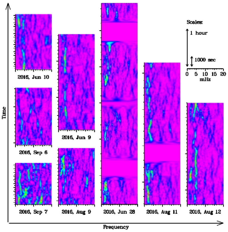
Figure 9: Stacked power spectra GS Pav in several nights after subtraction of variations on time scales longer than 12 min. The spectra are normalized to their nightly maxima and colour coded on a linear scale such that violet and red represent zero and maximum power, respectively. Spectral features within a range of 1000 sec (indicated by the length of the respective double arrow in the upper right of the figure) are not independent from each other. The horizontal violet bars in the spectra of 2016, June 28 and August 11 represent intervals without data (eclipses or interruptions of the observations). (For visualization of the colours used in this figure, the reader is referred to the web version of this article.)

During many of the nights conspicuous signals in the form of more or less continuous vertical streaks in the stacked power spectra in the range of approximately 2 - 5 mHz (500 - 200 sec), sometimes undulating somewhat in frequency, extend over periods of time well in excess of the independence limit. This behaviour may be most convincing on 2016, August 12 (rightmost spectrum of Fig. 9) where a signal centred at 4.8 mHz (208 sec) exends over more than half the light curve (lower part of the stacked spectrum) and is possibly resumed later on. On June 9 a signal appears with interruptions at 3.8 mHz (263 sec). Before the eclipse on August 11 there appears to be an oscillation at 2.3 mHz (435 sec), and immediately after the eclipse an oscillations which undulates between 3.9 mHz (256 sec) and 2.5 mHz (400 sec) can be discerned. Whether the signals later in that light curve should be considered as a continuation of the undulating oscillation or are due to isolated events is not clear. On June 10, the light curve starts with a significant signal at 4.7 mHz (212 sec), then appears to split into two branches, each of them being fainter than the original signal, only to join into a single oscillations of 4.4 mHz (227 sec), similar to the original one, at the end of the observations. During other nights, similar signals in the same frequency range appear, but is not as clear whether they represent QPOs or are just due to isolated flickering events.

Warner (2004) pointed out that QPOs are often observed in combination with DNOs. However an investigation of the high frequency part of the stacked power spectra of GS Pav (beyond the upper frequency limit shown in Fig. 9) did not reveal convincing evidence for DNOs. This is not surprising since the S/N ratio of the respective light curves is not better that of the EC 21178-5417 data where in spite of the detection by Warner et al. (2003) of a plethora of DNOs none could be seen (unless drawing on pre-information; not available in the case of GS Pav) possibly due to the insufficient S/N ratio.

5 V345 Pav

Most of what is known about V345 Pav (= EC 19314-5915) comes from a study of Buckley et al. (1992). They presented a detailed spectroscopic analysis, supplemented by some photometry. Based on eclipses observed in the latter they derived an orbital period of 4.7543 h. The spectrum of V345 Pav is peculiar in the sense that it exhibits metallic absorption lines typical of a G8 dwarf star which cannot be attributed to the secondary of the CV system. Instead, Buckley et al. (1992) conjectured the presence of a third star. As in the case of GS Pav, the initial motivation to include V345 Pav in the present study was the expectation to significantly improve the precision of the orbital period through observations of additional eclipses.

5.1 Eclipse timings and ephemeris

The minimum times of the 14 eclipses observed in V345 Pav were determined in the same way as for EC 21178-5417 and GS Pav. The typical error turned out to be 16.2 sec. The eclipse times are listed in Tab. 2 where eclipse no. #0 is arbitrarily assigned to the eclipse observed on 2015, May 22. These data permit to calculate preliminary ephemeris with sufficient precision to bridge the gap in time to the observations of Buckley et al. (1992) without cycle count ambiguity (negative eclipse numbers). As was the case for GS Pav, Buckley et al. (1992) list their eclipse timings of V345 Pav in HJD. Assuming that they also used the UTC time scale, I transformed them into BJD-TDB and include them in Table 2. Combining all eclipse timings then enables to calculate long-term ephemeris. The eclipses epochs of V345 Pav are given by:

$${\rm BJD_{min}} = 2457164.79433\ (20)$$

$$+0.1980963877\ (28)\times E$$

The rms-error of the residuals between the observed eclipse times and those calculated from these ephemeris is 23.8 sec. Again, the $O-C$ values for the individual eclipses are included in Table 2.

5.2 Eclipse profile

The light curves of V345 Pav can be separated into three distinct groups. The first one includes the observations of 2015 May and June, the second those of 2015, August, and the final one those of 2016, June. Fig. 10 (which is organized in a similar way as Fig. 2) shows the eclipse profiles of the three epochs. The graphs corresponding to 2015, August and 2016, June have been shifted downwards and upwards, respectively, by $0^{\raisebox{0.90417pt}{\scriptsize m}}_{\raisebox{1.80835pt}{\hskip 1.18999pt.}}3$ for clarity. While the eclipses of the first two epochs have been averaged (five eclipses of 2015, May – June and seven eclipses of 2015, August), the 2016, June eclipses are shown individually in order to visualize the significant difference in eclipse depth from one night to the next, while the out-of-eclipse level of the two light curves remained remarkably stable.

The deviations from symmetry of the eclipse profile is more pronounced in V345 Pav (in particular in 2015, May – June) than was observed in EC 21178-5417 and GS Pav but are qualitatively similar, again exhibiting a delayed hot spot egress. Additionally, the 2015 eclipses contain asymmetries in their mid-sections, when egress is steeper than ingress. Only the lower part of the eclipses appear perfectly symmetric.

The eclipse amplitudes, as gauged from the difference between the average magnitude in the phase intervals $-0.16<\phi<-0.14$ and $0.14<\phi<0.16$ and the minimum of a high order polynomial fit to the eclipse bottom, are listed in Table 3. The significantly larger scatter of the 2015, August eclipse depths (eclipse numbers 407 – 428) indicates that the system was in a much less stable state than during May-June when the eclipse depth was very stable.

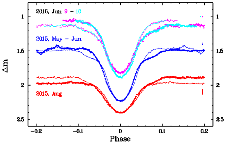
Figure 10: Eclipse profiles of V345 Pav: eclipses of 2016, June 9 (magenta) and 10 (cyan), both shifted upward by $0^{\raisebox{0.90417pt}{\scriptsize m}}_{\raisebox{1.80835pt}{\hskip 1.18999pt.}}3$ for clarity; average of five eclipses of 2015, May - June (blue); average of seven eclipses of 2015, August (red), shifted downward by $0^{\raisebox{0.90417pt}{\scriptsize m}}_{\raisebox{1.80835pt}{\hskip 1.18999pt.}}3$. For details of the organization of the figure, see Fig. 2. (For visualization of the colours used in this figure, the reader is referred to the web version of this article.)

The eclipses are shallower than in the other two targets of this study. This is due to the presence of the third star in the system. Buckley et al. (1992) estimate that it contributes 34% of the out-of-eclipse light in the $V$ band. Since the isophotal wavelength of our white light observations roughly correspond to $V$ (Bruch 2017) the expected eclipse depth in the absence of the third component can be calculated. Assuming that the percentage contribution of its light is constant (i.e., the out-of-eclipse variations are all due to uncertainties in the zero point of the differential magnitude scale between missions; see Sect. 2) the average depth during the three epochs of observation would then be $1^{\raisebox{0.90417pt}{\scriptsize m}}_{\raisebox{1.80835pt}{\hskip 1.18999pt.}}53$, $0^{\raisebox{0.90417pt}{\scriptsize m}}_{\raisebox{1.80835pt}{\hskip 1.18999pt.}}82$ and $1^{\raisebox{0.90417pt}{\scriptsize m}}_{\raisebox{1.80835pt}{\hskip 1.18999pt.}}55$.

5.3 Out-of-eclipses variations

Flickering in V345 Pav reaches only about half the amplitude that it attains in the other two targets of this study and is thus quite weak compared to most CVs. Again, data noise inhibits a more details quantitative investigation. In order to study the phase dependence of the out-of-eclipse variations, as in the previous cases the eclipses were first removed from the light curves. I distinguish between the 2015, May – June data and the light curves obtained in 2015, August. The data of June 12 were excluded from this analysis because they are much noisier than the rest, and those of August 10 because only a small part of the out-of-eclipse phases was observed. In order to remove slight night-to-night variations the average magnitude was subtracted from the individual nightly light curves which were then combined into two data sets, comprising the nights of May – June and of August, respectively. Finally, these data sets were folded on the orbital period.

The results are shown in Fig. 11. The 2015, May – June light curves appears to contain a faint orbital hump just before the eclipse at a phase when the classical hot spot is expected to rotate into view in cataclysmic variables. After the eclipse, the magnitude declines gradually to a minimum just before the onset of the hump. In contrast, in August V345 Pav attains an asymmetrically shaped maximum (the rise is steeper than the decline) roughly at phase $\phi=0.25$ and a minimum close to $\phi=0.82$, with the decline being interrupted by a smaller secondary maximum close to $\phi=0.6$. The increase in brightness across the eclipse is also clearly seen in Fig. 10. Note also that in agreement with the clear presence of the orbital hump in May-June and its absence in August the delayed hot spot eclipse egress is more pronounced in the first than in the second of these epochs (see Fig. 10). The overall time dependent behaviour of the out-of-eclipse variations again suggests the presence of an accretion disk with variable azimuthal structure leading to aspect dependent modulations in this high inclination system. The changing phase of the light curve maximum may serve as a warning against the perils to derive an orbital period (in the absence of eclipses) from repetitive (but only apparently periodic) brightness modulations alone.

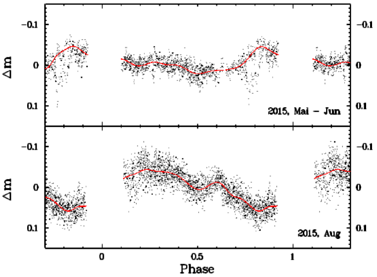
Figure 11: Phase folded out-of-eclipse light curves of V345 Pav of 2015, May – June (top) and August (bottom). The red lines are smoothed versions of the original data. (For visualization of the colours used in this figure, the reader is referred to the web version of this article.)

In order to verify the presence of periodic variations other than the orbital modulation Lomb-Scargle periodograms of the combined May-June and August light curves were calculated. They only contain sinals at the orbital frequency, its first overtone and their one/day aliases.

5.4 DNOs and QPOs

In contrast to EC 21178-5417, no previous information about the presence of DNOs, lpDNOs or QPOs is available for V345 Pav. I searched for such oscillations in the out-of-eclipse light curves in the same way as has been done in Sects. 3.4 and 4.4. While, again, the stacked power spectra contain a myrad of signals, none of them attains a false alarm probability low enough, extends beyond the independence limit, or repeats itself in  different nights to claim it as real with any degree of confidence. Therefore, I conclude that if oscillations are present in the data they remain below the detection limit. This is in agreement with Buckley et al. (1992) who also did not find evidence for DNOs or QSOs.

6 Conclusions

Time resolved photometry of three eclipsing novalike variables was investigated in order to (i) determine or to refine orbital ephemeris, (ii) quantify the properties of the eclipses, (iii) characterize the out-of-eclipse variations, and (iv) search of QPOs and DNOs. The longer time base over which the objects were observed, and – in the case of GS Pav and V345 Pav – combining them with published observations taken decades earlier, permitted to increase the precision of the period by one (GS Pav) to three (EC 21178-5417 and V345 Pav) orders of magnitude.

In all cases the eclipse profile is clearly structured, exhibiting a delay in late eclipse egress, i.e., the familiar feature caused by the egress of the hot spot on the accretion disk. Otherwise, the eclipses are symmetrical to a high degree. There depth exhibits significant variations on the time scale of weeks (i.e., between observing missions), but at least in GS Pav, variations occur also on shorter time scales. The same is true for the light level just before or after eclipse. In GS Pav, the correlation between out-of-eclipse brightness and eclipse depth observed by Groot et al. (1998) could not be confirmed. In view of the difficulty to measure precise contact phases (in particular during eclipse ingress) I resist the temptation to determine dynamical and geometric system properties using eclipse profiles.

Out of eclipse the variations remain modest but show some systematics. In all target stars flickering occurs only on a low scale with amplitudes restricted to $\sim$$0^{\raisebox{0.90417pt}{\scriptsize m}}_{\raisebox{1.80835pt}{\hskip 1.18999pt.}}1$ in EC 21178-5417 and GS Pav and $\sim$$0^{\raisebox{0.90417pt}{\scriptsize m}}_{\raisebox{1.80835pt}{\hskip 1.18999pt.}}05$ in V345 Pav. Superposed are systematic variations on longer time scales with a single maximum between phase 0.5 and 0.7 and an amplitude of $\approx$$0^{\raisebox{0.90417pt}{\scriptsize m}}_{\raisebox{1.80835pt}{\hskip 1.18999pt.}}25$ in EC 21178-4517, or a hump between phase 0.3 and 0.6 in addition to the classical hot spot hump just before eclipse (amplitudes: $0^{\raisebox{0.90417pt}{\scriptsize m}}_{\raisebox{1.80835pt}{\hskip 1.18999pt.}}1$ – $0^{\raisebox{0.90417pt}{\scriptsize m}}_{\raisebox{1.80835pt}{\hskip 1.18999pt.}}2$) in GS Pav. In V345 Pav the available data suggest that the pattern of out-of-eclipse variations is less stable on time scales of weeks or months. Apart from the described orbital variations at least in two nights GS Pav exhibits a periodicity on shorter time scales during time intervals of several hours. In one night a period of 15.7 min was measured, while in the next night it doubled (within the measurement error) to 30.2 min.

A multitude of QPOs and DNOs has been observed by Warner et al. (2003) in EC 21178-5417. These could not be retrieved in the present observations, probably because of a lower S/N ratio of the data. Only during one night (drawing on pre-information about the properties of these oscillations) possible indications for their presence were identified. A search for similar signals in V345 Pav was to no avail. However, in some light curves of GS Pav clear signs of persistent signals with somewhat modulated frequencies (corresponding to periods between 200 and 500 sec) and amplitudes were detected in stacked power spectra.

References

Beckemper, S. 1995, Statistische Untersuchungen zur Stärke des Flickering in kataklysmischen Veränderlichen, Diploma thesis, Münster

MIRA: A Reference Guide (Astron. Inst. Univ. Münster

Bruch, A. 2014, A&A, 566, A101

Bruch, A. 2016, New Astr., 46, 60

Bruch, A. 2017, New Astr., in press

Bruch, A., Diaz, M.P. 2017, New Astr., 50, 109

Buckley, D.A.H., O’Donoghue, D., Kilkenny, D., Stobie, S.R., & Remillard, R.A. 1992, MNRAS, 258,285

Deeming, T.J. 1975, Ap&SS, 39, 447

Eastman, J., Siverd, R., & Gaudi, B.S. 2010, PASP, 122, 935

Girard, T.M., Van Altena W.F., Zacharias, N., et al. 2011, AJ, 142, 15

Groot, P.J., Augusteijn, T., Barziv, O., & van Paradijs, J. 1998, A&A 340, L31

Hoffmeister, C. 1963, Veröff. Sternw. Sonneberg, 6, 1

Lomb, N.R. 1976, ApSS, 39, 447

Ritter, H., & Kolb, U. 2003, A&A, 404, 301

Scargle, J.D. 1982, ApJ, 263, 853

Schwarzenberg-Czerny, A. 1989, MNRAS, 241, 153

Stellingwerf, R.F. 1978, ApJ, 224, 953

Stobie, R.S., Kilkenny, D., O’Donoghue, D., et al. 1997, MNRAS, 287, 848

Warner, B. 2004, PASP, 116, 115

Warner, B., Woudt, P.A., & Pretorius, M.L. 2003, MNRAS, 344, 1193

Zacharias, N., Monet, D.G., Levine, S.E., et al. 2005, AAS, 205, 4815

Zacharias, N., Finch, C.T., Girard, T.M., et al. 2013, AJ, 145, 44

Zwitter, T., & Munari, U. 1995, A&AS, 114, 575