Robust Location-Aided Beam Alignment in Millimeter Wave Massive MIMO

Abstract

Among the enabling technologies for 5G wireless networks, millimeter wave (mmWave) communication offers the chance to deal with the bandwidth shortage affecting wireless carriers. Radio signals propagating in the mmWave band experience considerable path loss, leading to poor link budgets. As a consequence, large directive gains are needed in order to communicate and therefore, beam alignment stages have to be considered during the initial phases of the communication. While beam alignment is considered essential to the performance of such systems, it is also a costly operation in terms of latency and resources in the massive MIMO (mMIMO) regime due to the large number of beam combinations to be tested. Therefore, it is desirable to identify methods that allow to optimally trade-off overhead for performance. Location-aided beam training has been proposed recently as a possible solution to this problem, exploiting long-term spatial information so as to focus the beam search on particular areas, thus reducing overhead. However, due to mobility and other imperfections in the estimation process, the spatial information obtained at the base station (BS) and the user (UE) is likely to be noisy, degrading beam alignment performance. In this paper, we introduce a robust beam alignment framework in order to exhibit resilience with respect to this problem. We first recast beam alignment as a decentralized coordination problem where BS and UE seek coordination on the basis of correlated yet individual measurements. We formulate the optimum beam alignment solution as the solution of a Bayesian team decision problem. We then propose a suite of algorithms to approach optimal designs with reduced complexity. The effectiveness of the robust beam alignment procedure, compared with classical designs, is then verified on simulation settings with varying location information accuracies.

I Introduction

Millimeter wave communications (30-300 GHz) are receiving significant attention in 5G-related research, in the hope of unlocking the capacity bottleneck existing at sub-6 GHz bands [1]. The use of higher frequencies and higher bandwidths poses new implementation challenges, as for example in terms of hardware constraints or architectural features. Moreover, the propagation environment is adverse for smaller wavelength signals: compared with lower bands characteristics, diffraction tends to be lower while penetration or blockage losses can be much greater [2, 3, 4, 5]. Therefore, mmWave signals experience a severe path loss which hinders the establishment of a reliable communication link and requires the adoption of high-gain directional antennas or steerable antenna beams - i.e. beamforming is an absolute need [6].

On the upside, millimeter wavelengths allow to stack a high number of antenna elements in a modest space [7] thus making it possible to exploit the superior beamforming performance stemming from mMIMO arrays [8, 9, 10].

Rather than adopting complex digital beamforming – which might require unfeasible CSI-exchange due to the large number of channel dimensions in mMIMO arrays [9, 8, 10] – low cost mmWave communication architectures are suggested [11] where beam design is selected from discrete beam sets and then implemented in analog fashion. Another trend lies in the so-called hybrid beamforming architectures by which the effective dimension of the antenna space is reduced by a low-dimensional digital precoder, followed by an RF analog beamformer implemented using phase shifters [12, 13]. In all of these solutions, a bottleneck is found in the massive array regime while searching for the best beam combinations at transmitter and receiver which offer the best channel path, a problem referred to as beam alignment in the literature [14, 15, 16, 17]. This is especially true for communications between two mMIMO devices where the number of beam combinations is very large, representing a significant pilot and time resource overhead, in particular in applications demanding fast communication establishment [18].

The current literature reflects the interesting trade-off that is found in the problem of beam alignment between speed and beamforming performance. While narrower beamwidths lead to increased alignment overhead, they can provide a higher transmission rate once communication is established, as a result of higher directive gains and lower interference [17, 19]. On the other hand, larger beamwidths expedite the alignment process, though smaller beam gains reduce transmission rate and coverage [20, 21].

One approach for reducing alignment overhead – without compromising performance – has been proposed in [22]. It consists in exploiting device location side information so as to reduce the effective beam search areas in the presence of line of sight (LoS) propagation. Indeed, 5G devices (base station as well as terminal side) are expected to access ubiquitous location information – supported through a constellation of GNSS satellites providing positioning and timing data [23, 24]. Similar approaches are found in [25, 26, 27], where localization information – obtained through the use of radars, automotive sensors or out-of-band information – has been confirmed as a useful source of side information, capable of assisting link establishment in mmWave communications. Other beam alignment solutions based on localization information have been put forward for the high-speed train scenario [28] or for outdoor areas covered by Wi-Fi [29].

In this paper, we consider important limitation factors for location-aided beam alignment. First, user terminal and infrastructure side equipment are unlikely to acquire location information with the same degree of accuracy, for the following reasons. On one hand, the base station, being static, benefits from accurate information about its own position. In contrast the UE, being mobile, is harder to pinpoint by the BS. While, the UE can be expected to have more timely information about its own location, although unavoidably noisy. Moreover, practical propagation scenarios include settings with significant additional multipath created by dominant reflectors. The location information for such reflectors can be assumed to be available (via e.g. angle of arrival estimation), although with some uncertainty that is typically lower at the BS than at the UE.

We propose a framework for utilizing location side-information in a dual mMIMO setup (i.e. both UE and BS devices are equipped with possibly large arrays) while accounting for unequal levels of uncertainties on this information at the BS and at the UE sides. Our contributions are multi-fold:

1. Based on a probabilistic location information setting, we formulate a robust (Bayesian style) beam pre-selection problem. Because there are two devices (the BS and the UE) involved in making a beam pre-selection decision, we recast the problem as a decentralized team decision framework. The strength of the proposed approach lies in the fact that each device makes a beam decision that is weighed upon the quality of location information it has at its disposal and simultaneously on the quality level of location information expected at the other end.

2. We propose a family of algorithms, exploring various complexity-performance trade-off levels. We show how the devices decide to keep or drop path directions as a function of angle uncertainties (both locally and at the other link end) and average path energy.

II System Model

II-A Scenario

Consider the scenario in Figure 1. A transmitter (TX) with $N_{TX}\gg 1$ antennas seeks to establish communication with a single receiver (RX) with $N_{RX}\gg 1$ antennas. In order to extract the best possible combined TX-RX beamforming gain, the TX and the RX respectively aim to select a precoding vector $\mathbf{g}=\big{[}g_{1},g_{2},\dots,g_{N_{TX}}\big{]}^{\mathrm{T}}$, and a receive-side combining vector $\mathbf{w}=\big{[}w_{1},w_{2},\dots,w_{N_{RX}}\big{]}^{\mathrm{T}}$ from predefined codebooks. The codebooks include $M_{TX}$ and $M_{RX}$ beamforming vectors – i.e. beams – for the TX and the RX, respectively.

Optimal beam alignment consists in pilot-training every combination of TX and RX beams (out of $M_{TX}M_{RX}$) and selecting the pair which exhibits the highest signal to noise ratio. In the mMIMO regime, this requires prohibitive pilot, power and time resources. As a result, a method for pruning out unlikely beam combinations is desirable. To this end, we assume that the TX (resp. the RX) pre-selects a subset of $D_{TX}\ll M_{TX}$ (resp. $D_{RX}\ll M_{RX}$) beams for subsequent pilot training. When the pre-selection phase is over, the TX actively trains the pre-selected beams by sending pilots of each one of the $D_{TX}$ beams, while the RX is allowed to make SNR measurements over each of its $D_{RX}$ beams. Classically, communications can then take place over one (or more) of the pre-selected TX-RX beam combinations, such as e.g. the combination which maximizes the SNR. In this paper, we are interested in deriving beam subset pre-selection strategies that do not require any active channel sounding but can be carried out on the basis of long term statistical information including location-dependent information for the TX and the RX as introduced in [22]. In contrast with [22], we consider potential reflector location information and, in particular, we place the emphasis on robustness with respect to location uncertainties in a high-mobility scenario. Models for channels, long term location dependent information, and corresponding uncertainties are introduced in the following sections.

\begin{overpic}[trim=85.35826pt 227.62204pt 85.35826pt 227.62204pt,scale={0.785}]{./Graphics/Scenario} \put(16.6,33.5){\small{$BS$}} \put(81.0,35.5){\small{$UE$}} \put(53.0,55.5){\small{$R_{1}$}} \put(46.4,12.0){\small{$R_{2}$}} \end{overpic}

Figure 1: Scenario example for a given realization with $L=3$ channel paths.

II-B Channel Model

Based on recently reported data regarding the specular behavior of mmWave propagation channels [2, 3, 4, 5], we model the space-time channel with a limited number $L$ of dominant propagation paths, consisting of one LoS path and $L-1$ reflected paths.

The power-normalized $N_{RX}\times N_{TX}$ channel matrix $\mathbf{H}$ can thus be expressed as the sum of $L$ components or contributions [30, 13]:

$$\mathbf{H}=\big{(}N_{TX}N_{RX}\big{)}^{{}^{1}\!/_{2}}\Big{(}\sum_{\ell=1}^{L}\alpha_{\ell}\mathbf{a}_{RX}(\theta_{\ell})\mathbf{a}^{\mathrm{H}}_{TX}(\phi_{\ell})\Big{)}$$ (1)

where $\alpha_{\ell}\sim\mathcal{CN}(0,\sigma^{2}_{\ell})$ denotes the instantaneous random complex gain for the $\ell$-th path, having an average power $\sigma^{2}_{\ell},\ell=1,\dots,L$ such as $\sum\sigma^{2}_{\ell}=1$.

The variables $\phi_{\ell}\in[0,\pi]$ and $\theta_{\ell}\in[0,\pi]$ are the angles of departure (AoDs) and arrival (AoAs) for each path $\ell$, where one angle pair corresponds to the LoS direction while other might account for the presence of strong reflectors (buildings, hills) in the environment. The reflectors are denoted by $R_{i},i=1,\dots,L-1$ in the rest of the paper.

The vectors $\mathbf{a}_{TX}(\phi_{\ell})\in\mathbb{C}^{N_{TX}\times 1}$ and $\mathbf{a}_{RX}(\theta_{\ell})\in\mathbb{C}^{N_{RX}\times 1}$ denote the antenna response at the TX and the RX, respectively. For clarity of exposition, we will consider the popular example of critically-spaced uniform linear arrays (ULAs), we have [30]:

$$\mathbf{a}_{TX}(\phi_{\ell})=\frac{1}{(N_{TX})^{{}^{1}\!/_{2}}}\big{[}{1,e^{-i\pi\cos(\phi_{\ell})},\dots,e^{-i\pi(N_{TX}-1)\cos(\phi_{\ell})}}\big{]}^{\mathrm{T}}$$ (2)

$$\mathbf{a}_{RX}(\theta_{\ell})=\frac{1}{(N_{RX})^{{}^{1}\!/_{2}}}\big{[}{1,e^{-i\pi\cos(\theta_{\ell})},\dots,e^{-i\pi(N_{RX}-1)\cos(\theta_{\ell})}}\big{]}^{\mathrm{T}}$$ (3)

II-C Beam Codebook

We denote the transmit and receive beam codebooks as:

$$\mathcal{V}_{TX}=\{\mathbf{g}_{1},\dots,\mathbf{g}_{M_{TX}}\},\quad\mathcal{V}_{RX}=\{\mathbf{w}_{1},\dots,\mathbf{w}_{M_{RX}}\}.$$ (4)

For ULAs, a suitable design for the fixed beam vectors in the codebook consists in selecting steering vectors over a discrete grid of angles [11, 16, 27]:

$$\mathbf{g}_{p}=\mathbf{a}_{TX}(\bar{\phi}_{p}),\quad p\in\{1,\dots,M_{TX}\}$$ (5)

$$\mathbf{w}_{q}=\mathbf{a}_{RX}(\bar{\theta}_{q}),\quad q\in\{1,\dots,M_{RX}\}$$ (6)

where the angles $\bar{\phi}_{p},p\in\{1,\dots,M_{TX}\}$ and $\bar{\theta}_{q},q\in\{1,\dots,M_{RX}\}$ can be chosen according to different strategies, including regular and non regular sampling of the $[0,\pi]$ range (see details in Section V-A).

III Information Model

As discussed in the introduction, we are interested in the exploitation of long-term statistical (including location-dependent) information, to perform beam pre-selection (i.e. choosing $D_{TX}$ and $D_{RX}$). Unlike prior work, the emphasis of this work lies in the accounting for uncertainties in the acquisition of such information respectively at the base station and the user terminal. In what follows we introduce the information model emphasizing the decentralized nature of information available at TX and RX sides.

III-A Definition of the Model

In order to establish a reference case, we consider the setting where the available information lets us exactly characterize the average rate (i.e. knowing the SNR) that would be obtained under any choice of TX and RX beams. To this end, we define the average beam gain matrix.

Definition 1.

The average beam gain matrix $\mathbf{G}\in\mathbb{R}^{M_{RX}\times M_{TX}}$ contains the power level associated with each combined choice of transmit-receive beam pair after averaging over small scale fading. It is defined as:

$$G_{q,p}=\mathbb{E}_{\bm{\alpha}}\big{[}|\mathbf{w}^{\mathrm{H}}_{q}\mathbf{H}\mathbf{g}_{p}|^{2}\big{]}$$ (7)

where the expectation is carried out over the channel coefficients $\bm{\alpha}=[\alpha_{1},\alpha_{2},\dots,\alpha_{L}]$ and with $G_{q,p}$ denoting the $(q,p)$-element of $\mathbf{G}$.

Definition 2.

The position matrix $\mathbf{P}\in\mathbb{R}^{2\times(L+1)}$ contains the two-dimensional location coordinates $\mathbf{p}_{u}=[p_{u_{x}}\quad p_{u_{y}}]^{\mathrm{T}}$ for node $u$, where $u$ indifferently refers to either the TX (or BS), the RX (or UE) or one of the reflectors $R_{i},i=1,\dots,L-1$. It is defined as follows:

$$\mathbf{P}=\begin{bmatrix}\mathbf{p}_{TX}&\mathbf{p}_{R_{1}}&\dots&\mathbf{p}_{R_{L-1}}&\mathbf{p}_{RX}\end{bmatrix}$$ (8)

The following lemma characterizes the gain matrix $\mathbf{G}$ as a function of the position matrix $\mathbf{P}$ in the configuration considered above.

Lemma 1.

We can write the average beam gain matrix as follows:

$$G_{q,p}(\mathbf{P})=\sum_{\ell=1}^{L}\sigma_{\ell}^{2}|L_{RX}(\Delta_{\ell,q})|^{2}|L_{TX}(\Delta_{\ell,p})|^{2}$$ (9)

where we remind the reader that $\sigma_{\ell}^{2}$ denotes the variance of the channel coefficients $\alpha_{\ell}$ and we have defined:

$$L_{TX}(\Delta_{\ell,p}) =\frac{1}{(N_{TX})^{{}^{1}\!/_{2}}}\frac{e^{i(\pi/2)\Delta_{\ell,p}}}{e^{i(\pi/2)N_{TX}\Delta_{\ell,p}}}\frac{\sin((\pi/2)N_{TX}\Delta_{\ell,p})}{\sin((\pi/2)\Delta_{\ell,p})}$$ (10)

$$L_{RX}(\Delta_{\ell,q}) =\frac{1}{(N_{RX})^{{}^{1}\!/_{2}}}\frac{e^{i(\pi/2)\Delta_{\ell,q}}}{e^{i(\pi/2)N_{RX}\Delta_{\ell,q}}}\frac{\sin((\pi/2)N_{RX}\Delta_{\ell,q})}{\sin((\pi/2)\Delta_{\ell,q})}$$ (11)

and

$$\Delta_{\ell,p}=(\cos(\bar{\phi}_{p})-\cos(\phi_{\ell}))$$ (12)

$$\Delta_{\ell,q}=(\cos(\theta_{\ell})-\cos(\bar{\theta}_{q}))$$ (13)

with the angles $\phi_{\ell},\ell=1,\dots,L$ and $\theta_{\ell},\ell=1,\dots,L$ obtained from the position matrix $\mathbf{P}$ using simple algebra (the detailed steps are relegated to the Appendix for the sake of readability).

Note that it is possible to ignore the second terms in (10) and (11), as we aim to compute the squared absolute value in (9).

III-B Distributed Noisy Information Model

Since the actual position matrix is unlikely to be available, neither at the BS nor at the UE, we introduce a noisy location-based information model upon which beam pre-selection will be carried out.

In a realistic setting where both BS and UE separately acquire location information via a noisy process of GNSS-based estimation, angle of arrival estimation (for reflector position estimation) and latency-prone BS-UE feedback, a distributed noisy position information model ensues whereby positioning accuracy is device dependent (i.e. different at BS and UE).

Noisy information model at the TX: The noisy position matrix $\mathbf{\hat{P}}^{(TX)}$ available at the TX is modeled as:

$$\mathbf{\hat{P}}^{(TX)}=\mathbf{P}+\mathbf{E}^{(TX)}$$ (14)

where $\mathbf{E}^{(TX)}$ denotes the following matrix:

$$\mathbf{E}^{(TX)}=\begin{bmatrix}\mathbf{e}^{(TX)}_{TX}&\mathbf{e}^{(TX)}_{R_{1}}&\dots&\mathbf{e}^{(TX)}_{R_{L-1}}&\mathbf{e}^{(TX)}_{RX}&\end{bmatrix}$$ (15)

containing the random position estimation error made by TX on $\mathbf{p}_{u}$, with an arbitrary, yet known, probability density function $f_{\mathbf{e}^{(TX)}_{u}}$.

Noisy information model at RX: Akin to the TX side, the receiver obtains the estimate $\mathbf{\hat{P}}^{(RX)}$, where:

$$\mathbf{\hat{P}}^{(RX)}=\mathbf{P}+\mathbf{E}^{(RX)}$$ (16)

where $\mathbf{E}^{(RX)}$ is defined as $\mathbf{E}^{(TX)}$ in (15), but containing the random position estimation error made by RX on $\mathbf{p}_{u}$, with a known distribution $f_{\mathbf{e}^{(RX)}_{u}}$.

Note that we assume $\mathbf{e}^{(TX)}_{TX}=\mathbf{e}^{(RX)}_{TX}=0$, which indicates that the position information of the static BS is known perfectly by all.

III-C Shared Information

In what follows the number of dominant path $L$, and their average path powers $\sigma^{2}_{l},l=1,\dots,L$ are assumed to be known by both BS and UE based on prior averaged measurements. Similarly, statistical distributions $f_{\mathbf{e}^{(TX)}_{u}},f_{\mathbf{e}^{(RX)}_{u}}$ are supposed to be quasi-static and as such are supposed to be available (or estimated) to both BS and UE. In other words, the BS (resp. the UE) is aware of the quality for position estimates which it and the UE (resp. BS) have at their disposal. For instance, typically, the BS might know less about the UE location than the UE itself, e.g. due to latency in communicating UE position to the BS in a highly mobile scenario or due to the use of different position technologies (GPS at the UE, LTE TDOA localization at the BS). In contrast, the BS might have greater capabilities to estimate the position of the reflectors accurately compared to the UE, due to a larger number of antennas at the BS or due to interactions with multiple UEs. Both the BS and UE are aware of this situation and might wish to exploit it for greater coordination performance. The central question of this paper is “how?”.

\begin{overpic}[trim=108.12054pt 227.62204pt 85.35826pt 227.62204pt,scale={0.55}]{Tx_Scen} \end{overpic}

(a) View at TX

\begin{overpic}[trim=108.12054pt 227.62204pt 85.35826pt 227.62204pt,scale={0.55}]{Rx_Scen} \end{overpic}

(b) View at RX

Figure 2: Use case of interest for a given realization with $L=3$. Approximate position information is denoted with blue (TX) and orange (RX) points, along with their uncertainty circles, with respect to black points representing actual positions. Here, a bounded error model is assumed.

IV Coordinated Beam Alignment Methods

In this section, we present strategies for coordinated beam alignment which aim at restoring robustness in the beam pre-selection phase in the face of an arbitrary amount of uncertainty (noise) as shown in equations (14), (16).

Let $\mathcal{D}_{TX}$ (resp. $\mathcal{D}_{RX}$) be the set of $D_{TX}=|\mathcal{D}_{TX}|$ (resp. $D_{RX}=|\mathcal{D}_{RX}|$) pre-selected beams at the TX (resp. the RX).

In order to choose the beams, we will use the following figure of merit $\mathbb{E}[R(\mathcal{D}_{TX},\mathcal{D}_{RX},\mathbf{P})]$, where:

$$R(\mathcal{D}_{TX},\mathcal{D}_{RX},\mathbf{P})=\max_{p\in\mathcal{D}_{TX},q\in\mathcal{D}_{RX}}\log_{2}\Big{(}1+\frac{G_{q,p}(\mathbf{P})}{N_{0}}\Big{)}$$ (17)

where $N_{0}$ is the thermal noise power and the average gain is obtained from the position matrix $\mathbf{P}$ as shown in Lemma 1.

IV-A Beam Alignment under Perfect Information

Before introducing the distributed approaches to this problem, we focus on the idealized benchmark, where both the TX and the RX obtain the perfect position matrix $\mathbf{P}$.

The beam sets $(\mathcal{D}^{\textrm{up}}_{TX},\mathcal{D}^{\textrm{up}}_{RX})$ which maximize the transmission rate are then found as follows:

$$(\mathcal{D}^{\textrm{up}}_{TX},\mathcal{D}^{\textrm{up}}_{RX})=\operatorname*{argmax}_{\mathcal{D}_{TX}\subset\mathcal{V}_{TX},\mathcal{D}_{RX}\subset\mathcal{V}_{RX}}R\big{(}\mathcal{D}_{TX},\mathcal{D}_{RX},\mathbf{P}\big{)}.$$ (18)

IV-B Optimal Bayesian Beam Alignment

Let us now consider the core of this work whereby the TX and the RX must make beam pre-selection decisions in a decentralized manner, based on their respective location information in (14) and (16), respectively. Interestingly, this problem can be recast as a so-called team decision theoretic problem [32, 33] where team members (here TX and RX) seek to coordinate their actions so as to maximize overall system performance, while not being able to accurately predict each other decision due to noisy observations. For instance, with $D_{TX}=D_{RX}=2$, the TX might decide to beam in the direction of the RX and Reflector 1, while the RX might decide to beam in the direction of the TX but also Reflector 2 (for example, if its information on the position of Reflector 1 is not accurate enough). As a result, a strong mismatch would be obtained for one of the pre-selected beam pairs. The goal of the robust decentralized algorithm is hence to avoid such inefficient behavior.

Beam pre-selection at the TX is equivalent to a mapping:

$$\begin{aligned} \mathit{d}_{TX}:\quad&\mathbb{R}^{2\times(L+1)}\rightarrow\mathcal{V}_{TX}\\ &\mathbf{\hat{P}}^{(TX)}\mapsto\mathit{d}_{TX}(\mathbf{\hat{P}}^{(TX)})\end{aligned}$$ (19)

and at the RX, we have the following mapping:

$$\begin{aligned} \mathit{d}_{RX}:\quad&\mathbb{R}^{2\times(L+1)}\rightarrow\mathcal{V}_{RX}\\ &\mathbf{\hat{P}}^{(RX)}\mapsto\mathit{d}_{RX}(\mathbf{\hat{P}}^{(RX)})\end{aligned}$$ (20)

Let $\mathcal{S}$ denote the space containing all possible choices of pairs of such functions.

The optimally-robust team decision strategy $(\mathit{d}_{TX}^{*}$, $\mathit{d}_{RX}^{*})\in\mathcal{S}$ maximizing the expected rate reads as follows:

$$(\mathit{d}_{TX}^{*},\mathit{d}_{RX}^{*})=\operatorname*{argmax}_{(\mathit{d}_{TX},\mathit{d}_{RX})\in\mathcal{S}}\mathbb{E}_{\mathbf{P},\mathbf{\hat{P}}^{(TX)},\mathbf{\hat{P}}^{(RX)}}\Big{[}R\big{(}\mathit{d}_{TX}(\mathbf{\hat{P}}^{(TX)}),\mathit{d}_{RX}(\mathbf{\hat{P}}^{(RX)}),\mathbf{P}\big{)}\Big{]}$$ (21)

where the expectation operator is carried out over the joint pdf $f_{\mathbf{P},\mathbf{\hat{P}}^{(TX)},\mathbf{\hat{P}}^{(RX)}}$.

The optimization in (21) is a stochastic functional optimization problem which is notoriously difficult to directly solve [34].

In order to circumvent this problem, we now examine strategies which offer an array of trade-offs between the optimal robustness of (21) and the implementation complexity.

IV-C Naive Beam Alignment

A simple, yet naive, implementation of decentralized coordination mechanisms consists in having each side making its decision by treating (mistaking) local information as perfect and global. Thus, TX and RX solve for (18), where the TX assumes $\mathbf{\hat{P}}^{TX}=\mathbf{P}$ and the RX considers $\mathbf{\hat{P}}^{RX}=\mathbf{P}$. We denote the resulting mappings as $(\mathit{d}_{TX}^{\textrm{naive}},\mathit{d}_{RX}^{\textrm{naive}})\in\mathcal{S}$, which are found as follows:

• Optimization at TX:

  $$\mathit{d}_{TX}^{\textrm{naive}}(\mathbf{\hat{P}}^{(TX)})=\operatorname*{argmax}_{\mathcal{D}_{TX}\subset\mathcal{V}_{TX}}\operatorname*{\phantom{g}max}_{\mathcal{D}_{RX}\subset\mathcal{V}_{RX}}R\big{(}\mathcal{D}_{TX},\mathcal{D}_{RX},\mathbf{\hat{P}}^{(TX)}\big{)}$$ (22)

• Optimization at RX:

  $$\mathit{d}_{RX}^{\textrm{naive}}(\mathbf{\hat{P}}^{(RX)})=\operatorname*{argmax}_{\mathcal{D}_{RX}\subset\mathcal{V}_{RX}}\operatorname*{\phantom{g}max}_{\mathcal{D}_{TX}\subset\mathcal{V}_{TX}}R\big{(}\mathcal{D}_{TX},\mathcal{D}_{RX},\mathbf{\hat{P}}^{(RX)}\big{)}$$ (23)

which can be solved by exhaustive set search or a lower complexity greedy approach (see details later). The basic limitation of the naive approach in (22) and (23) is that it fails to account for either (i) the noise in the gain matrix estimate at the decision maker, or (ii) the differences in location information quality between the TX and the RX. Indeed, the TX (resp. RX) assumes that the RX (resp. TX) receives the same estimate and take its decision on this basis, which is represented by the maximization inside the equations (22) and (23).

IV-D 1-Step Robust Beam Alignment

Making one step towards robustness requires from the TX and the RX to account for their own local information noise statistics. As a first approximation for robustness, each device might assume that its local estimate, while not perfect, is at least globally shared, i.e. that $\mathbf{\hat{P}}^{(TX)}=\mathbf{\hat{P}}^{(RX)}$ for the purpose of algorithm derivation. We denote the resulting beam pre-selection as 1-step robust – obtained through the following mappings $(\mathit{d}_{TX}^{\textrm{1-s}},\mathit{d}_{RX}^{\textrm{1-s}})\in\mathcal{S}$:

• Optimization at TX:

  $$\mathit{d}_{TX}^{\textrm{1-s}}(\mathbf{\hat{P}}^{(TX)})=\operatorname*{argmax}_{\mathcal{D}_{TX}\subset\mathcal{V}_{TX}}\operatorname*{\phantom{g}max}_{\mathcal{D}_{RX}\subset\mathcal{V}_{RX}}\mathbb{E}_{\mathbf{P}|\mathbf{\hat{P}}^{(TX)}}\Big{[}R\big{(}\mathcal{D}_{TX},\mathcal{D}_{RX},\mathbf{P}\big{)}\Big{]}$$ (24)

• Optimization at RX:

  $$\mathit{d}_{RX}^{\textrm{1-s}}(\mathbf{\hat{P}}^{(RX)})=\operatorname*{argmax}_{\mathcal{D}_{RX}\subset\mathcal{V}_{RX}}\operatorname*{\phantom{g}max}_{\mathcal{D}_{TX}\subset\mathcal{V}_{TX}}\mathbb{E}_{\mathbf{P}|\mathbf{\hat{P}}^{(RX)}}\Big{[}R\big{(}\mathcal{D}_{TX},\mathcal{D}_{RX},\mathbf{P}\big{)}\Big{]}$$ (25)

Optimization (21) is therefore replaced with a more standard stochastic optimization problem for which a vast literature is available (see [35] for a nice overview). Considering w.l.o.g. the optimization at the TX, one standard approach consists in approximating the expectation by Monte-Carlo runs according to the probability density function $f_{\mathbf{P}|\mathbf{\hat{P}}^{(TX)}}$. Once the expectation operator has been replaced by a discrete summation, the optimal solution of the discrete optimization problem can be simply again obtained by greedy search. Indeed, the nature of the problem is such that it is possible to split (24) and (25) in multiple maximizations – over the single beams in $\mathcal{V}_{TX}$ and $\mathcal{V}_{RX}$ – without loosing optimality. The proposed 1-step robust approach is summarized in Algorithm 1 (showing what is done at TX side). The RX runs the same algorithm with inputs $\mathbf{\hat{P}}^{(RX)}$ and $f_{\mathbf{e}^{(RX)}_{u}}$  $\forall u$, where in line 5 the max is instead operated over columns.

Algorithm 1 1-Step Robust Beam Alignment (TX side)

1:INPUT: $\mathbf{\hat{P}}^{(TX)}$, $f_{\mathbf{e}^{(TX)}_{u}}$  $\forall u$

2:for $i=1:M$ do $\triangleright$ Approximate expectation over $\mathbf{P}|\mathbf{\hat{P}}^{(TX)}$ with $M$ Monte-Carlo iterations

3:    Compute possible position matrix $\mathbf{\hat{P}}=\mathbf{\hat{P}}^{(TX)}-\mathbf{\hat{E}}$, with $\mathbf{\hat{E}}$ generated according to $f_{\mathbf{e}^{(TX)}_{u}}$  $\forall u$

4:    Compute possible gain matrix $\mathbf{\hat{G}}$ through (34) and (47)

5:    $\mathbf{M}(:,i)=\max(\mathbf{\hat{G}},\mathrm{``rows"})$ $\triangleright$ Find the max for each column

6:end for

7:$\mathrm{Idx}=\mathrm{sort}(\mathrm{mean}(\mathbf{M},\mathrm{``columns"}),\mathrm{``descending"})$ $\triangleright$ Order the beams after averaging over the for loop

8:$\mathcal{D}_{TX}=\mathrm{Idx}(1:D_{TX})$ $\triangleright$ The first $D_{TX}$ beams are pre-selected for pilot transmission

The greedy approach has far less complexity than the exhaustive search, which requires to search over beam sets whose size is the number of combinations resulting from picking $D_{TX}$ (resp. $D_{RX}$) beams at a time among $M_{TX}$ (resp. $M_{RX}$).

Note that the approach above provides robustness with respect to the local noise at the decision maker; it however fails to account for discrepancies in location information quality across TX and RX. Indeed, the true distribution of the position knowledge has been approximated by considering that both the TX and the RX share the same information.

IV-E 2-Step Robust Beam Alignment

A necessary optimality condition for the optimal Bayesian beam alignment in (21) is that it is person-by-person optimal, i.e. each node takes the best strategy given the strategy at the other node [34]. The person-by-person optimal solution $(\mathit{d}_{TX}^{\textrm{PP}},\mathit{d}_{RX}^{\textrm{PP}})\in\mathcal{S}$ satisfies the following system of fixed point equations:

• Optimization at TX:

  $$\mathit{d}_{TX}^{\textrm{PP}}(\mathbf{\hat{P}}^{(TX)})=\operatorname*{argmax}_{\mathcal{D}_{TX}\subset\mathcal{V}_{TX}}\mathbb{E}_{\mathbf{P},\mathbf{\hat{P}}^{(RX)}|\mathbf{\hat{P}}^{(TX)}}\Big{[}R\big{(}\mathcal{D}_{TX},\mathit{d}^{\textrm{PP}}_{RX}(\mathbf{\hat{P}}^{(RX)}),\mathbf{P}\big{)}\Big{]}$$ (26)

• Optimization at RX:

  $$\mathit{d}_{RX}^{\textrm{PP}}(\mathbf{\hat{P}}^{(RX)})=\operatorname*{argmax}_{\mathcal{D}_{RX}\subset\mathcal{V}_{RX}}\mathbb{E}_{\mathbf{P},\mathbf{\hat{P}}^{(TX)}|\mathbf{\hat{P}}^{(RX)}}\Big{[}R\big{(}\mathit{d}^{\textrm{PP}}_{TX}(\mathbf{\hat{P}}^{(TX)}),\mathcal{D}_{RX},\mathbf{P}\big{)}\Big{]}$$ (27)

Still, the interdependence between (26) and (27) makes solving this system of equations challenging. Thus, we propose an approximate solution in which this dependence is removed by replacing the person-by-person mapping inside the expectation operator with the 1-step robust mapping described in Section IV-D.

Intuitively, the TX (resp. the RX) finds its strategy by using the belief that the RX (resp. the TX) is using the 1-step robust strategy (which can be separately computed thanks to (24), (25)) and seeking to be (2-step) robust with respect to remaining uncertainties. In the 2-step algorithm, both local noise statistics and differences between information quality at TX and RX are thus exploited. Let us denote by $(\mathit{d}_{TX}^{\textrm{2-s}},\mathit{d}_{RX}^{\textrm{2-s}})\in\mathcal{S}$ the 2-step robust approach, which reads as:

• Optimization at TX:

  $$\mathit{d}_{TX}^{\textrm{2-s}}(\mathbf{\hat{P}}^{(TX)})=\operatorname*{argmax}_{\mathcal{D}_{TX}\subset\mathcal{V}_{TX}}\mathbb{E}_{\mathbf{P},\mathbf{\hat{P}}^{(RX)}|\mathbf{\hat{P}}^{(TX)}}\Big{[}R\big{(}\mathcal{D}_{TX},\mathit{d}^{\textrm{1-s}}_{RX}(\mathbf{\hat{P}}^{(RX)}),\mathbf{P}\big{)}\Big{]}$$ (28)

• Optimization at RX:

  $$\mathit{d}_{RX}^{\textrm{2-s}}(\mathbf{\hat{P}}^{(RX)})=\operatorname*{argmax}_{\mathcal{D}_{RX}\subset\mathcal{V}_{RX}}\mathbb{E}_{\mathbf{P},\mathbf{\hat{P}}^{(TX)}|\mathbf{\hat{P}}^{(RX)}}\Big{[}R\big{(}\mathit{d}^{\textrm{1-s}}_{TX}(\mathbf{\hat{P}}^{(TX)}),\mathcal{D}_{RX},\mathbf{P}\big{)}\Big{]}$$ (29)

The proposed 2-step algorithm is summarized in Algorithm 2 (showing what is done at TX side).

Remark 1.

This approach could then be extended by inserting the 2-step robust mapping inside the expectation operator, so as to get the 3-step robust approach, and so forth. Of course, it comes with an increased computational cost. ∎

Algorithm 2 2-Step Robust Beam Alignment (TX side)

1:INPUT: $\mathbf{\hat{P}}^{(TX)}$, $f_{\mathbf{e}^{(TX)}_{u}}$, $f_{\mathbf{e}^{(RX)}_{u}}$  $\forall u$

2:for $i=1:M$ do $\triangleright$ Approximate expectation over $\mathbf{P}|\mathbf{\hat{P}}^{(TX)}$ with $M$ Monte-Carlo iterations

3:    Compute possible position matrix $\mathbf{\hat{P}}=\mathbf{\hat{P}}^{(TX)}-\mathbf{\hat{E}}$, with $\mathbf{\hat{E}}$ generated according to $f_{\mathbf{e}^{(TX)}_{u}}$  $\forall u$

4:    Compute possible gain matrix $\mathbf{\hat{G}}$ through (34) and (47)

5:    for $k=1:M$ do $\triangleright$ Approximate expectation over $\mathbf{\hat{P}}^{(RX)}|\mathbf{\hat{P}}^{(TX)}$ with $M$ Monte-Carlo iterations

6:         Compute possible position matrix $\mathbf{\hat{\hat{P}}}=\mathbf{\hat{P}}+\mathbf{\hat{\hat{E}}}$, with $\mathbf{\hat{E}}$ generated according to $f_{\mathbf{e}^{(RX)}_{u}}$  $\forall u$

7:         Compute possible gain matrix $\mathbf{\hat{\hat{G}}}$ through (34) and (47)

8:         $\mathbf{\tilde{M}}(:,k)=\max(\mathbf{\hat{\hat{G}}},\mathrm{``columns"})$ $\triangleright$ Find the max for each row

9:    end for

10:    $\mathrm{Idx}=\mathrm{sort}(\mathrm{mean}(\mathbf{\tilde{M}},\mathrm{``columns"}),\mathrm{``descending"})$ $\triangleright$ Order the beams after averaging over the for loop

11:    $\mathbf{M}(:,i)=\max(\mathbf{\hat{G}}(\mathrm{Idx}(1:B_{RX}),:),\mathrm{``rows"})$ $\triangleright$ Find the max over the columns associated to $\mathit{d}^{\textrm{1-s}}_{RX}$

12:end for

13:$\mathrm{Idx}=\mathrm{sort}(\mathrm{mean}(\mathbf{M},\mathrm{``columns"}),\mathrm{``descending"})$ $\triangleright$ Order the beams after averaging over the for loop

14:$\mathcal{D}_{TX}=\mathrm{Idx}(1:D_{TX})$ $\triangleright$ The first $D_{TX}$ beams are pre-selected for pilot transmission

V Simulation Results

In this section, numerical results are presented so as to compare the performance of the proposed beam alignment algorithms. We consider the scenario in Fig. 1, with $L=3$ multipath components. A distance of $100$ m is assumed from the TX to the RX. Both TX and RX are equipped with $N_{TX}=N_{RX}=64$ antennas (ULA). The devices have to choose $D_{TX}$, $D_{RX}$ beamforming vectors among the $M_{TX}=M_{RX}=64$ in the codebooks, as discussed in Section II-A. The results are averaged over $10000$ independent Monte-Carlo iterations.

V-A Beam Codebook Design

Since ULAs produce unequal beamwidths according to the pointing direction – wider through the endfire direction, tighter through the broadside direction, as it can be seen in Figure 1 – we separate the grid angles $\bar{\phi}_{p}$ and $\bar{\theta}_{q}$ according to the inverse cosine function, as follows [22]:

$$\bar{\phi}_{p}=\arccos\Big{(}1-\frac{2(p-1)}{M_{TX}-1}\Big{)},\quad p\in\{1,\dots,M_{TX}\}$$ (30)

$$\bar{\theta}_{q}=\arccos\Big{(}1-\frac{2(q-1)}{M_{RX}-1}\Big{)},\quad q\in\{1,\dots,M_{RX}\}$$ (31)

As a result, and in order to guarantee almost equal gain losses among the adjacent angles, more of the latter are considered as the broadside direction is reached.

V-B Location Information Model

In the simulations, we use a uniform bounded error model for location information [22]. In particular, we assume that all the estimates lie somewhere inside disks centered in the actual positions $\mathbf{p}_{u},u\in\{TX,RX,R_{i}\},i=1,\dots,L-1$. Let $S(r)$ be the two-dimensional closed ball centered at the origin and of radius $r$, i.e. $S(r)=\{\mathbf{p}\in\mathbb{R}^{2}:\lVert{\mathbf{p}}\rVert\leq r\}$. We model the random estimation errors as follows:

• $\mathbf{e}_{u}^{(TX)}$ uniformly distributed in $S(r_{u}^{(TX)})$

• $\mathbf{e}_{u}^{(RX)}$ uniformly distributed in $S(r_{u}^{(RX)})$

such that $r_{u}^{(TX)}$ and $r_{u}^{(RX)}$ are the maximum positioning error for node $u$ as seen from the TX and the RX, respectively.

V-C Results and Discussion

According to measurement campaigns [2, 3, 4, 5], LoS propagation is the prominent propagation driver in mmWave bands. We consider as a consequence a stronger (on average) LoS path, with respect to the reflected paths. The latter are assumed to have the same average power. Moreover, we consider the following degrees of precision for localization information:

• $r_{RX}^{(TX)}=13$ m, $r_{RX}^{(RX)}=7$ m

• $r_{R_{1}}^{(TX)}=11$ m, $r_{R_{1}}^{(RX)}=18$ m

• $r_{R_{2}}^{(TX)}=15$ m, $r_{R_{2}}^{(RX)}=17$ m

• $r_{TX}^{(TX)}=0$ m, $r_{TX}^{(RX)}=0$ m

In general, those values are tied together so that it is unrealistic to have e.g. small uncertainties for the reflectors (reflecting points) associated to relatively big uncertainties for the RX. Indeed, the location of the reflecting point depends on the location of the devices.

Given that 5G devices are expected to access position information with a guaranteed precision of about $1$ m in open areas [23], those settings are robust with respect to the mobility of the devices or to possible discontinuous location awareness.

Fig. 3 compares the proposed algorithms in the settings described above, which we define as the set of parameters $\mathcal{A}$. It can be seen that the 2-step robust beam alignment outperforms the other distributed solutions, being able to consider statistical information at both ends.

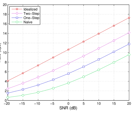
Figure 3: Rate vs SNR, stronger LoS path, parameters $\mathcal{A}$, $D_{TX}=D_{RX}=4$.

In Fig. 4, we consider the performance of the proposed algorithms as a function of the number of pre-selected beams – assuming a fixed SNR of 10 dB, and the same parameters as considered for Fig. 3.

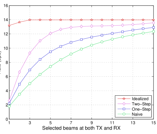
Figure 4: Rate vs number of pre-selected beams at TX and RX (among $M_{TX}=M_{RX}=64$), parameters $\mathcal{A}$, for a given SNR $=10$ dB.

As expected, a higher number of pre-selectable beams leads to increased performance. Simulations show that the 2-step robust algorithm almost reaches the centralized approach with already $D_{TX}=D_{RX}=5$. This is due to its ability to focus the beam search on the angular directions related to the stronger LoS path, at both TX and RX sides.

In addition, Fig. 4 confirms that exploiting position information allows to reduce alignment overhead while impacting only slightly on the performance if the sets of pre-selectable beams are sufficiently large with respect to the degrees of precision.

In order to understand the actual behaviour of the proposed algorithms, we plot in Figure 6(b) the pre-selected beams for a given realization.

It is also interesting to observe how the proposed algorithms behave in case of LoS blockage. We consider thus an LoS path with $\sigma^{2}_{\textrm{LoS}}=0$, and reflected paths with the same average power. Moreover, we consider another set of degrees of precision for localization information, as follows:

• $r_{RX}^{(TX)}=7$ m, $r_{RX}^{(RX)}=3$ m

• $r_{R_{1}}^{(TX)}=8$ m, $r_{R_{1}}^{(RX)}=11$ m

• $r_{R_{2}}^{(TX)}=18$ m, $r_{R_{2}}^{(RX)}=8$ m

• $r_{TX}^{(TX)}=0$ m, $r_{TX}^{(RX)}=0$ m

We will denote this additional group of settings as the set of parameters $\mathcal{B}$.

In this case as well, as it can be seen in Fig. 5, the 2-step robust algorithm outperforms the other distributed solutions, with a slightly smaller gap compared to the case with settings $\mathcal{A}$, due to the higher accuracy of localization information.

The chosen beams in case of settings $\mathcal{B}$ can be seen in Fig. 7(b) for a given realization.

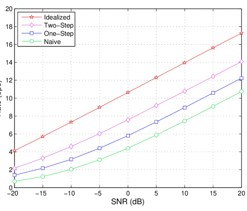
Figure 5: Rate vs SNR, stronger LoS path, parameters $\mathcal{B}$, $D_{TX}=D_{RX}=4$.

\begin{overpic}[trim=71.13188pt 142.26378pt 14.22636pt 156.49014pt,scale={0.475}]{./Graphics/BeamFormers_PerKnow_Param5} \end{overpic}

(a) Idealized BA

\begin{overpic}[trim=71.13188pt 142.26378pt 14.22636pt 156.49014pt,scale={0.475}]{./Graphics/BeamFormers_Naive_Param5} \end{overpic}

(b) Naïve BA

\begin{overpic}[trim=71.13188pt 142.26378pt 14.22636pt 199.16928pt,scale={0.475}]{./Graphics/BeamFormers_TR_Param5} \end{overpic}

(d) 2-Step Robust BA

Figure 6: Beams chosen for pilot transmission by the proposed algorithms, for a given realization, with $L=3$, one stronger path (LoS) ($\sigma^{2}_{\textrm{LoS}}=0.4$ as shown), parameters $\mathcal{A}$ and $D_{TX}=D_{RX}=7$.

\begin{overpic}[trim=71.13188pt 142.26378pt 14.22636pt 199.16928pt,scale={0.475}]{./Graphics/BeamFormers_Rm_Param5} \end{overpic}

(c) 1-Step Robust BA

\begin{overpic}[trim=71.13188pt 142.26378pt 14.22636pt 156.49014pt,scale={0.475}]{./Graphics/BeamFormers_PerKnow_Param7} \end{overpic}

(a) Idealized BA

\begin{overpic}[trim=71.13188pt 142.26378pt 14.22636pt 156.49014pt,scale={0.475}]{./Graphics/BeamFormers_Naive_Param7} \end{overpic}

(b) Naïve BA

\begin{overpic}[trim=71.13188pt 142.26378pt 14.22636pt 199.16928pt,scale={0.475}]{./Graphics/BeamFormers_TR_Param7} \end{overpic}

(d) 2-Step Robust BA

Figure 7: Beams chosen for pilot transmission by the proposed algorithms, for a given realization, with $L=3$, LoS blockage ($\sigma^{2}_{\textrm{LoS}}=0$ as shown), parameters $\mathcal{B}$ and $D_{TX}=D_{RX}=4$.

\begin{overpic}[trim=71.13188pt 142.26378pt 14.22636pt 199.16928pt,scale={0.475}]{./Graphics/BeamFormers_Rm_Param7} \end{overpic}

(c) 1-Step Robust BA

VI Conclusions

Localization information plays an important role in reducing alignment overhead in mmWave communications. Dealing with the imperfect position knowledge is challenging due to the fact that the information is not shared between the TX and the RX, leading to disagreements affecting the performance. In this work, we introduced an algorithm which takes into account the imperfect information at both ends and improves the coordination between the TX and the RX by exploiting their shared statistical knowledge of localization errors.

We proposed a so-called 2-step robust approach which enforce coordination by letting one node assume a given strategy for the other one, thus strongly reducing complexity.

Numerical experiments have shown that good performance can be achieved with the 2-step robust algorithm, which almost reaches the idealized upper bound – obtained with perfect information – even with small values of pre-selectable beams.

Future directions include the extension of the proposed algorithms, in order to exceed the 2-step algorithm, with the purpose of reaching the person-by-person optimum. Finding closed forms of the proposed algorithms is an interesting and challenging research problem which is still open as well.

VII Acknowledgment

F. Maschietti, D. Gesbert, P. de Kerret are supported by the ERC under the European Union’s Horizon 2020 research and innovation program (Agreement no. 670896).

Derivation of Lemma 1. Starting from the obtained channel gain, for a given pair of beamforming vectors as defined in (5) and (6), we have:

$$|\mathbf{w}^{\mathrm{H}}_{q}\mathbf{H}\mathbf{g}_{p}|^{2} =\Big{|}\big{(}N_{TX}N_{RX}\big{)}^{{}^{1}\!/_{2}}\sum_{\ell=1}^{L}\alpha_{\ell}\big{(}\mathbf{w}^{\mathrm{H}}(\bar{\theta}_{q})\mathbf{a}_{RX}(\theta_{\ell})\big{)}\big{(}\mathbf{a}^{\mathrm{H}}_{TX}(\phi_{\ell})\mathbf{g}(\bar{\phi}_{p})\big{)}\Big{|}^{2}$$ (32)

$$=\Big{|}\big{(}N_{TX}N_{RX}\big{)}^{{}^{1}\!/_{2}}\sum_{\ell=1}^{L}\alpha_{\ell}\big{(}\frac{1}{N_{RX}}\sum_{m=0}^{N_{RX}-1}e^{-i\pi m\Delta_{\ell,q}}\big{)}\big{(}\frac{1}{N_{TX}}\sum_{n=0}^{N_{TX}-1}e^{-i\pi n\Delta_{\ell,p}}\big{)}\Big{|}^{2}$$ (33)

with $\Delta_{\ell,q}=(\cos(\theta_{\ell})-\cos(\bar{\theta}_{q}))$ and $\Delta_{\ell,p}=(\cos(\bar{\phi}_{p})-\cos(\phi_{\ell}))$.

We used the following formula to calculate the angle $\phi$ between the line connecting two points $\mathbf{p}=[p_{x}\quad p_{y}]$ and $\mathbf{q}=[q_{x}\quad q_{y}]$, and the vertical line $x=q_{x}$ passing through the point $\mathbf{q}$:

$$\phi=\frac{\pi}{2}-\arctan\Big{(}\frac{p_{x}-q_{x}}{p_{y}-q_{y}}\Big{)}$$ (34)

for which $\phi\in[0,\pi]$. Equation (34) can be used to derive actual or estimated AoDs/AoAs, starting from $\mathbf{P}$, $\mathbf{\hat{P}}^{(TX)}$ and $\mathbf{\hat{P}}^{(RX)}$. For example, the AoDs $\phi_{\ell}~{}\forall\ell$ can be computed as follows:

$$\phi_{\ell}=\frac{\pi}{2}-\arctan\Big{(}\frac{p_{u_{x}}-p_{{TX}_{x}}}{p_{u_{y}}-p_{{TX}_{y}}}\Big{)},\quad u\in\{RX,R_{i}\},i=1,\dots,L-1$$ (35)

while the AoAs $\theta_{\ell}~{}\forall\ell$ as:

$$\theta_{\ell}=\frac{\pi}{2}-\arctan\Big{(}\frac{p_{u_{x}}-p_{{RX}_{x}}}{p_{u_{y}}-p_{{RX}_{y}}}\Big{)},\quad u\in\{TX,R_{i}\},i=1,\dots,L-1$$ (36)

According to our definition in (34), the AoDs are evaluated from north to south, while the opposite is done for the AoAs.

The sums which appear in (32) are the sums of the first $N_{RX}$ and $N_{TX}$ terms of the geometric series with ratio $e^{-i\pi\Delta_{\ell,q}}$ and $e^{-i\pi\Delta_{\ell,p}}$. We can thus write:

$$|\mathbf{w}^{\mathrm{H}}_{q}\mathbf{H}\mathbf{g}_{p}|^{2} =\Big{|}\sum_{\ell=1}^{L}\alpha_{\ell}\big{(}\frac{1}{(N_{RX})^{{}^{1}\!/_{2}}}\frac{1-e^{-i\pi N_{RX}\Delta_{\ell,q}}}{1-e^{-i\pi\Delta_{\ell,q}}}\big{)}\big{(}\frac{1}{(N_{TX})^{{}^{1}\!/_{2}}}\frac{1-e^{-i\pi N_{TX}\Delta_{\ell,p}}}{1-e^{-i\pi\Delta_{\ell,p}}}\big{)}\Big{|}^{2}$$ (37)

$$\stackrel{{\scriptstyle(a)}}{{=}}\Big{|}\sum_{\ell=1}^{L}\alpha_{\ell}\big{(}\frac{1}{(N_{RX})^{{}^{1}\!/_{2}}}\frac{1-\frac{e^{-i(\pi/2)N_{RX}\Delta_{\ell,q}}}{e^{i(\pi/2)N_{RX}\Delta_{\ell,q}}}}{1-\frac{e^{-i(\pi/2)\Delta_{\ell,q}}}{e^{i(\pi/2)\Delta_{\ell,q}}}}\big{)}\big{(}\frac{1}{(N_{TX})^{{}^{1}\!/_{2}}}\frac{1-\frac{e^{-i(\pi/2)N_{TX}\Delta_{\ell,p}}}{e^{i(\pi/2)N_{TX}\Delta_{\ell,p}}}}{1-\frac{e^{-i(\pi/2)\Delta_{\ell,p}}}{e^{i(\pi/2)\Delta_{\ell,p}}}}\big{)}\Big{|}^{2}$$ (38)

$$\!\!\stackrel{{\scriptstyle(b)}}{{=}}\!\Big{|}\sum_{\ell=1}^{L}\!\alpha_{\ell}\big{(}\frac{1}{(N_{RX})^{{}^{1}\!/_{2}}}\frac{\frac{e^{i(\pi/2)N_{RX}\Delta_{\ell,q}}-e^{-i(\pi/2)N_{RX}\Delta_{\ell,q}}}{e^{i(\pi/2)N_{RX}\Delta_{\ell,q}}}}{\frac{e^{i(\pi/2)\Delta_{\ell,q}}-e^{-i(\pi/2)\Delta_{\ell,q}}}{e^{i(\pi/2)\Delta_{\ell,q}}}}\big{)}\big{(}\frac{1}{(N_{TX})^{{}^{1}\!/_{2}}}\frac{\frac{e^{i(\pi/2)N_{TX}\Delta_{\ell,p}}-e^{-i(\pi/2)N_{TX}\Delta_{\ell,p}}}{e^{i(\pi/2)N_{TX}\Delta_{\ell,p}}}}{\frac{e^{i(\pi/2)\Delta_{\ell,p}}-e^{-i(\pi/2)\Delta_{\ell,p}}}{e^{i(\pi/2)\Delta_{\ell,p}}}}\big{)}\Big{|}^{2}$$ (39)

where $(a)$ and $(b)$ come from basic algebra. From (39), we get:

$$|\mathbf{w}^{\mathrm{H}}_{q}\mathbf{H}\mathbf{g}_{p}|^{2}= \Big{|}\sum_{\ell=1}^{L}\alpha_{\ell}\big{(}\frac{1}{(N_{RX})^{{}^{1}\!/_{2}}}\frac{e^{i(\pi/2)\Delta_{\ell,q}}}{e^{i(\pi/2)N_{RX}\Delta_{\ell,q}}}\frac{e^{i(\pi/2)N_{RX}\Delta_{\ell,q}}-e^{-i(\pi/2)N_{RX}\Delta_{\ell,q}}}{e^{i(\pi/2)\Delta_{\ell,q}}-e^{-i(\pi/2)\Delta_{\ell,q}}}\big{)}\cdots$$

$$\ \cdots\big{(}\frac{1}{(N_{TX})^{{}^{1}\!/_{2}}}\frac{e^{i(\pi/2)\Delta_{\ell,p}}}{e^{i(\pi/2)N_{TX}\Delta_{\ell,p}}}\frac{e^{i(\pi/2)N_{TX}\Delta_{\ell,p}}-e^{-i(\pi/2)N_{TX}\Delta_{\ell,p}}}{e^{i(\pi/2)\Delta_{\ell,p}}-e^{-i(\pi/2)\Delta_{\ell,p}}}\big{)}\Big{|}^{2}$$ (40)

Since $\sin(x)=(e^{ix}-e^{-ix})/2i$, (VII) results in:

$$|\mathbf{w}^{\mathrm{H}}_{q}\mathbf{H}\mathbf{g}_{p}|^{2}= \Big{|}\sum_{\ell=1}^{L}~{}\alpha_{\ell}\big{(}\frac{1}{(N_{RX})^{{}^{1}\!/_{2}}}\frac{e^{i(\pi/2)\Delta_{\ell,q}}}{e^{i(\pi/2)N_{RX}\Delta_{\ell,q}}}\frac{\sin((\pi/2)N_{RX}\Delta_{\ell,q})}{\sin((\pi/2)\Delta_{\ell,q})}\big{)}\cdots$$

$$\ \cdots\big{(}\frac{1}{(N_{TX})^{{}^{1}\!/_{2}}}\frac{e^{i(\pi/2)\Delta_{\ell,p}}}{e^{i(\pi/2)N_{TX}\Delta_{\ell,p}}}\frac{\sin((\pi/2)N_{TX}\Delta_{\ell,p})}{\sin((\pi/2)\Delta_{\ell,p})}\big{)}\Big{|}^{2}$$ (41)

From (VII), we can express the gain matrix $\mathbf{G}$ as follows:

$$\mathbf{G}_{q,p}=\mathbb{E}_{\bm{\alpha}}\big{[}\big{|}\sum_{\ell=1}^{L}\alpha_{\ell}L_{RX}(\Delta_{\ell,q})L_{TX}(\Delta_{\ell,p})\big{|}^{2}\big{]}$$ (42)

where we defined:

$$L_{TX}(\Delta_{\ell,p}) =\frac{1}{(N_{TX})^{{}^{1}\!/_{2}}}\frac{e^{i(\pi/2)\Delta_{\ell,p}}}{e^{i(\pi/2)N_{TX}\Delta_{\ell,p}}}\frac{\sin((\pi/2)N_{TX}\Delta_{\ell,p})}{\sin((\pi/2)\Delta_{\ell,p})}$$ (43)

$$L_{RX}(\Delta_{\ell,q}) =\frac{1}{(N_{RX})^{{}^{1}\!/_{2}}}\frac{e^{i(\pi/2)\Delta_{\ell,q}}}{e^{i(\pi/2)N_{RX}\Delta_{\ell,q}}}\frac{\sin((\pi/2)N_{RX}\Delta_{\ell,q})}{\sin((\pi/2)\Delta_{\ell,q})}$$ (44)

Equation (42) is rewritten as follows:

$$\mathbf{G}_{q,p}=\mathbb{E}_{\bm{\alpha}}\big{[}\big{(}\sum_{\ell=1}^{L}\alpha_{\ell}L_{RX}(\Delta_{\ell,q})L_{TX}(\Delta_{\ell,p})\big{)}\big{(}\sum_{\ell=1}^{L}\alpha_{\ell}L_{RX}(\Delta_{\ell,q})L_{TX}(\Delta_{\ell,p})\big{)}^{\mathrm{H}}\big{]}$$ (45)

$$\stackrel{{\scriptstyle(a)}}{{=}}\mathbb{E}_{\bm{\alpha}}\big{[}\big{(}\sum_{\ell=1}^{L}|\alpha_{\ell}|^{2}|L_{RX}(\Delta_{\ell,q})|^{2}|L_{TX}(\Delta_{\ell,p})|^{2}\big{)}\big{]}$$ (46)

$$=\sum_{\ell=1}^{L}\sigma_{\ell}^{2}|L_{RX}(\Delta_{\ell,q})|^{2}|L_{TX}(\Delta_{\ell,p})|^{2}$$ (47)

where $(a)$ comes from the statistical independence of the path gains $\alpha_{\ell}$. ∎

References

- [1] R. W. Heath, N. González-Prelcic, S. Rangan, W. Roh, and A. M. Sayeed, “An overview of signal processing techniques for millimeter wave MIMO systems,” IEEE J. Sel. Topics Signal Process., Apr. 2016.
- [2] I. Rodriguez, H. C. Nguyen, T. B. Sorensen, J. Elling, J. A. Holm, P. Mogensen, and B. Vejlgaard, “Analysis of 38 GHz mmWave propagation characteristics of urban scenarios,” in Proc. of European Wireless Conf., May 2015.
- [3] P. F. M. Smulders and L. M. Correia, “Characterisation of propagation in 60 GHz radio channels,” Electron. Commun. Eng. J., Apr. 1997.
- [4] H. Zhang, S. Venkateswaran, and U. Madhow, “Channel modeling and MIMO capacity for outdoor millimeter wave links,” in IEEE Wireless Commun. and Netw. Conf., Apr. 2010.
- [5] T. S. Rappaport, F. Gutierrez, E. Ben-Dor, J. N. Murdock, Y. Qiao, and J. I. Tamir, “Broadband millimeter-wave propagation measurements and models using adaptive-beam antennas for outdoor urban cellular communications,” IEEE Trans. Antennas Propag., Apr. 2013.
- [6] S. Wyne, K. Haneda, S. Ranvier, F. Tufvesson, and A. F. Molisch, “Beamforming effects on measured mm-wave channel characteristics,” IEEE Trans. Wireless Commun., Nov. 2011.
- [7] B. Biglarbegian, M. Fakharzadeh, D. Busuioc, M. R. Nezhad-Ahmadi, and S. Safavi-Naeini, “Optimized microstrip antenna arrays for emerging millimeter-wave wireless applications,” IEEE Trans. Antennas Propag., May 2011.
- [8] W. Roh, J. Y. Seol, J. Park, B. Lee, J. Lee, Y. Kim, J. Cho, K. Cheun, and F. Aryanfar, “Millimeter-wave beamforming as an enabling technology for 5G cellular communications: theoretical feasibility and prototype results,” IEEE Commun. Mag., Feb. 2014.
- [9] F. Rusek, D. Persson, B. K. Lau, E. G. Larsson, T. L. Marzetta, O. Edfors, and F. Tufvesson, “Scaling up MIMO: Opportunities and challenges with very large arrays,” IEEE Signal Process. Mag., Jan. 2013.
- [10] L. Lu, G. Y. Li, A. L. Swindlehurst, A. Ashikhmin, and R. Zhang, “An overview of massive MIMO: Benefits and challenges,” IEEE J. Sel. Topics Signal Process., Oct. 2014.
- [11] J. Wang, Z. Lan, C. W. Pyo, T. Baykas, C. S. Sum, M. A. Rahman, R. Funada, I. Lakkis, H. Harada, and S. Kato, “Beam codebook based beamforming protocol for multi-gbps millimeter-wave WPAN systems,” in IEEE Global Telecommun. Conf. (GLOBECOM), Nov. 2009.
- [12] F. Sohrabi and W. Yu, “Hybrid digital and analog beamforming design for large-scale antenna arrays,” IEEE J. Sel. Topics Signal Process., Apr. 2016.
- [13] A. Alkhateeb, O. E. Ayach, G. Leus, and R. W. Heath, “Channel estimation and hybrid precoding for millimeter wave cellular systems,” IEEE J. Sel. Topics Signal Process., Oct. 2014.
- [14] S. Haghighatshoar and G. Caire, “The beam alignment problem in mmWave wireless networks,” in Asilomar Conf. on Signals, Syst. and Comput., Nov. 2016.
- [15] A. Alkhateeb, Y. H. Nam, M. S. Rahman, C. Zhang, and R. W. Heath, “Initial beam association in millimeter wave cellular systems: Analysis and design insights,” IEEE Trans. Wireless Commun., Feb. 2017.
- [16] S. Hur, T. Kim, D. J. Love, J. V. Krogmeier, T. A. Thomas, and A. Ghosh, “Millimeter wave beamforming for wireless backhaul and access in small cell networks,” IEEE Trans. Commun., Oct. 2013.
- [17] H. Shokri-Ghadikolaei, L. Gkatzikis, and C. Fischione, “Beam-searching and transmission scheduling in millimeter wave communications,” in IEEE Int. Conf. on Commun. (ICC), June 2015.
- [18] M. Simsek, A. Aijaz, M. Dohler, J. Sachs, and G. Fettweis, “5G-enabled tactile internet,” IEEE J. Sel. Areas Commun., Mar. 2016.
- [19] S. Singh, R. Mudumbai, and U. Madhow, “Interference analysis for highly directional 60-GHz mesh networks: The case for rethinking medium access control,” IEEE/ACM Trans. on Netw., Oct. 2011.
- [20] H. Shokri-Ghadikolaei, C. Fischione, G. Fodor, P. Popovski, and M. Zorzi, “Millimeter wave cellular networks: A MAC layer perspective,” IEEE Trans. Commun., Oct. 2015.
- [21] M. Giordani, M. Mezzavilla, C. N. Barati, S. Rangan, and M. Zorzi, “Comparative analysis of initial access techniques in 5G mmWave cellular networks,” in Annual Conf. on Inform. Science and Syst. (CISS), Mar. 2016.
- [22] N. Garcia, H. Wymeersch, E. G. Ström, and D. Slock, “Location-aided mm-wave channel estimation for vehicular communication,” in IEEE Int. Workshop on Signal Process. Advances in Wireless Commun. (SPAWC), Jul. 2016.
- [23] R. D. Taranto, S. Muppirisetty, R. Raulefs, D. Slock, T. Svensson, and H. Wymeersch, “Location-aware communications for 5G networks: How location information can improve scalability, latency, and robustness of 5G,” IEEE Signal Process. Mag., Nov. 2014.
- [24] C. J. Hegarty and E. Chatre, “Evolution of the Global Navigation Satellite System (GNSS),” Proc. IEEE, Dec. 2008.
- [25] J. Choi, V. Va, N. González-Prelcic, R. Daniels, C. R. Bhat, and R. W. Heath, “Millimeter-wave vehicular communication to support massive automotive sensing,” IEEE Commun. Mag., Dec. 2016.
- [26] N. González-Prelcic, R. Méndez-Rial, and R. W. Heath, “Radar aided beam alignment in mmWave V2I communications supporting antenna diversity,” in Inf. Theory and Appl. Workshop (ITA), Jan. 2016.
- [27] A. Ali, N. González-Prelcic, and R. W. Heath, “Millimeter wave beam-selection using out-of-band spatial information,” Feb. 2017. [Online]. Available: http://arxiv.org/abs/1702.08574
- [28] V. Va, X. Zhang, and R. W. Heath, “Beam switching for millimeter wave communication to support high speed trains,” in IEEE Veh. Technology Conf., Sept. 2015.
- [29] A. S. A. Mubarak, E. M. Mohamed, and H. Esmaiel, “Millimeter wave beamforming training, discovery and association using WiFi positioning in outdoor urban environment,” in Int. Conf. on Microelectron. (ICM), Dec. 2016.
- [30] A. M. Sayeed, “Deconstructing multiantenna fading channels,” IEEE Trans. Signal Process., Oct. 2002.
- [31] A. Alkhateeb, G. Leus, and R. W. Heath, “Limited feedback hybrid precoding for multi-user millimeter wave systems,” IEEE Trans. Wireless Commun., Nov 2015.
- [32] Y.-C. Ho and K.-C. Chu, “Team decision theory and information structures in optimal control problems,” IEEE Trans. Autom. Control, Feb. 1972.
- [33] R. Radner, “Team decision problems,” The Annals of Mathematical Statistics, Sept. 1962.
- [34] P. de Kerret, S. Lasaulce, D. Gesbert, and U. Salim, “Best-response team power control for the interference channel with local CSI,” in IEEE Int. Conf. on Commun. (ICC), June 2015.
- [35] A. Shapiro, D. Dentcheva, and A. Ruszczyński, Lectures on stochastic programming: modeling and theory. Society for Industrial and Applied Mathematics, 2014.