Minimal Dispersion Approximately Balancing Weights:
Asymptotic Properties and Practical Considerations

Abstract

Weighting methods are widely used to adjust for covariates in observational studies, sample surveys, and regression settings. In this paper, we study a class of recently proposed weighting methods which find the weights of minimum dispersion that approximately balance the covariates. We call these weights minimal weights and study them under a common optimization framework. The key observation is the connection between approximate covariate balance and shrinkage estimation of the propensity score. This connection leads to both theoretical and practical developments. From a theoretical standpoint, we characterize the asymptotic properties of minimal weights and show that, under standard smoothness conditions on the propensity score function, minimal weights are consistent estimates of the true inverse probability weights. Also, we show that the resulting weighting estimator is consistent, asymptotically normal, and semiparametrically efficient. From a practical standpoint, we present a finite sample oracle inequality that bounds the loss incurred by balancing more functions of the covariates than strictly needed. This inequality shows that minimal weights implicitly bound the number of active covariate balance constraints. We finally provide a tuning algorithm for choosing the degree of approximate balance in minimal weights. We conclude the paper with four empirical studies that suggest approximate balance is preferable to exact balance, especially when there is limited overlap in covariate distributions. In these studies, we show that the root mean squared error of the weighting estimator can be reduced by as much as a half with approximate balance.

Keywords: Causal Inference; Missing Data; Observational Study; Sample Surveys; Weighting.

1 Introduction

1.1 Weighting methods for covariate adjustment

Weighting methods are widely used to adjust for observed covariates, for example in observational studies of causal effects (Rosenbaum, 1987), in sample surveys and panel data with unit non-response (Robins et al., 1994), and in regression settings with missing and/or mismeasured covariates (Hirano et al., 2003). Weighting methods are popular because they do not require explicitly modeling the outcome (Rosenbaum, 1987). As a result, they are part of the design stage as opposed to the analysis stage of the study (Rubin, 2008), which helps to maintain the objectivity of the study and preserve the validity of its tests (Rosenbaum, 2010). Furthermore, weighting methods are considered to be multipurpose in the sense that one set of weights can be used to estimate the mean of multiple outcomes (Little and Rubin, 2014).

Conventionally, the weights are estimated by modeling the propensities of receiving treatment or exhibiting missingness and then inverting the predicted propensities. However, with this approach it can be difficult to properly adjust for or balance the observed covariates. The reason is that this approach only balances covariates in expectation, by the law of large numbers, but in any particular data set it can be difficult to balance covariates, especially if the data set is small or if the covariates are sparse (Zubizarreta et al., 2011). In addition, this approach can result in very unstable estimates when a few observations have very large weights (e.g., Kang and Schafer 2007). To address these problems, a number of methods have been proposed recently. Instead of explicitly modeling the propensities of treatment or missingness, these methods directly balance the covariates. Some of these methods also minimize a measure of dispersion of the weights. Examples include Hainmueller (2012), Zubizarreta (2015), Chan et al. (2016), Zhao and Percival (2017), Wong and Chan (2018), and Zhao (2018). Earlier and related methods include Deville and Särndal (1992), Hellerstein and Imbens (1999), Imai and Ratkovic (2014), and Li et al. (2018). Two promising methods that use similar weights together with outcome information are Athey et al. (2018) and Hirshberg and Wager (2018). See Yiu and Su (2018) for a framework for constructing weights such that the association between the covariates and the treatment assignment is eliminated after weighting.

Most of these weighting methods balance covariates exactly rather than approximately. This is a subtle but important difference because approximate balance can trade bias for variance whereas exact balance cannot. Also, exact balance may not admit a solution whereas approximate balance may do so. For a fixed sample size, approximate balance may balance more functions of the covariates than exact balance.

In this paper, we study the class of weights of minimum dispersion that approximately balance the covariates. We call these weights minimal dispersion approximately balancing weights, or simply minimal weights. While it has been shown that instances of minimal weights work well in practice in both low- and high-dimensional settings (e.g., Zubizarreta 2015; Athey et al. 2018; Hirshberg and Wager 2018), and there are valuable theoretical results (e.g., Athey et al. 2018; Hirshberg and Wager 2018; Wong and Chan 2018), important aspects of their theoretical properties and their practical usage remain to be studied.

1.2 Theoretical properties and practical considerations of minimal weights

In this paper, we study the class of minimal weights. The key observation is the connection between approximate covariate balance and shrinkage estimation of the propensity score. This connection leads to both theoretical and practical developments.

From a theoretical standpoint, we first establish a connection between minimal weights and shrinkage estimation of the propensity score. We show that the dual of the minimal weights optimization problem is similar to parameter estimation in generalized linear models under $\ell_{1}$ regularization. This connection allows us to establish the asymptotic properties of minimal weights by leveraging results on propensity score estimation. In particular, we show that under standard smoothness conditions minimal weights are consistent estimates of the true inverse probability weights both in the $\ell_{2}$ and $\ell_{\infty}$ norms.

Next we study the asymptotic properties of a linear estimator based on minimal weights. We show that the weighting estimator is consistent, asymptotically normal, and semiparametrically efficient. This result is related to Chan et al. (2016), Fan et al. (2016), Zhao and Percival (2017), and Zhao (2018) in that it establishes the asymptotic optimality of a similar weighting estimator. It differs, however, in that it encompasses both approximate balance and exact balance. The technical conditions required by this result are among the weakest in the literature: they are considerably weaker than those required by Hirano et al. (2003) and Chan et al. (2016), and are comparable to those by Fan et al. (2016).

From a practical standpoint, we address two problems in minimal weights: choosing the number of basis functions and selecting the degree of approximate balance. We derive a finite-sample upper bound for the potential loss incurred by balancing too many basis functions of the covariates. This result shows that the loss due to balancing too many basis functions is hedged by minimal weights because the number of active balancing constraints is implicitly bounded.

We finally provide a tuning algorithm for calibrating the degree of approximate balance in minimal weights. This is a general problem in weighting and thus this algorithm can be of independent interest. We conclude with four empirical studies that suggest approximate balance is preferable to exact balance, especially when there is limited overlap in covariate distributions. These studies show that approximate balancing weights with the proposed tuning algorithm yields weighting estimators with considerably lower root mean squared error than their exact balancing counterparts.

2 A shrinkage estimation view of minimal weights

For simplicity of exposition, we focus on the problem of estimating a population mean from a sample with incomplete outcome data. We assume the outcomes are missing at random (Little and Rubin, 2014). Under the closely related assumption of strong ignorability (Rosenbaum and Rubin, 1983), this problem is analogous to estimating an average treatment effect in an observational study (see Kang and Schafer 2007 for an example). See Kang and Schafer (2007) for an example connecting the problems of causal inference and estimation with incomplete outcome data.

Consider a random sample of $n$ units from a population of interest, where some of the units in the sample are missing due to nonresponse. Let $Z_{i}$ be the response indicator with $Z_{i}=1$ if unit $i$ responds and $Z_{i}=0$ otherwise, $i=1,\ldots,n$. Write $r$ for the total number of respondents. Denote $X_{i}$ as the (vector of) observed covariates of unit $i$ and $Y_{i}$ as the outcome.

Assume there is overlap; that is, the propensity score $\pi(x)=\mathrm{pr}(Z=1\mid X=x)$ satisfies $0<\pi(x)<1.$ Furthermore, assume that the responses are missing at random. This assumption states that missingness can be fully explained by the observed covariates: $Y_{i}\mathchoice{\mathrel{\hbox to0.0pt{$\displaystyle\perp$\hss}\mkern 2.0mu{\displaystyle\perp}}}{\mathrel{\hbox to0.0pt{$\textstyle\perp$\hss}\mkern 2.0mu{\textstyle\perp}}}{\mathrel{\hbox to0.0pt{$\scriptstyle\perp$\hss}\mkern 2.0mu{\scriptstyle\perp}}}{\mathrel{\hbox to0.0pt{$\scriptscriptstyle\perp$\hss}\mkern 2.0mu{\scriptscriptstyle\perp}}}Z_{i}\,|\,X_{i}$ (Robins and Gill, 1997).

The goal is to estimate the population mean of the outcome $\bar{Y}=E(Y_{i})$. We use the linear estimator $\hat{Y}_{w}=\sum^{n}_{i=1}w_{i}Z_{i}Y_{i}$ for estimation, where the weights $w_{i}$ adjust for or balance the observed covariates.

Conventionally, the weights $w_{i}$ are obtained by fitting a model for the propensity score $\pi(x)$ and then inverting the predicted propensities. Despite being widely used, this approach has two problems in practice: first, balancing the covariates can be difficult due to misspecification of the propensity score model, if the sample size is small, or if the covariates are sparse; second, the weighting estimator can be unstable due to the variability of the weights (see, e.g., Zubizarreta 2015 for a discussion).

To address these problems, several weighting methods have been proposed recently. These methods are encompassed by the following mathematical program

$$\underset{\bm{w}}{\text{minimize}} \sum^{n}_{i=1}Z_{i}f(w_{i}) (1.1)$$ (1)

subject to $$\left|\sum^{n}_{i=1}w_{i}Z_{i}B_{k}(X_{i})-\frac{1}{n}\sum^{n}_{i=1}B_{k}(X_{i})\right|\leq\delta_{k},\>k=1,\ldots,K \hskip 8.82028pt(1.2)$$

where $f$ is a convex function of the weights, and $B_{k}(X_{i}),k=1,\ldots,K$, are smooth functions of the covariates. Typically, the functions $B_{k}$ are basis functions for $E(Y_{i})$ and are chosen as the moments of the covariate distributions (see assumptions 1.4 and 1.6 below). Other common choices of $B_{k}$ include spline (De Boor, 1972) and wavelet bases (Singh and Tiwari, 2006). The constants $\delta_{k}$ constrain the imbalances in $B_{k}$. They are summarized in the vector $\delta_{K\times 1}=(\delta_{1},\ldots,\delta_{K})\geq 0$. In (1.2), we can also constrain the weights to sum to one, $\sum^{n}_{i=1}w_{i}=1$, and to take positive values, $0\leq w_{i}$, $i=1,\ldots,n$. These two constraints together ensure that the weights do not extrapolate; that is, $0\leq w_{i}\leq 1,i=1,\ldots,n$. This is related to the sample boundedness property discussed by Robins et al. (2007), which requires the estimator to lie within the range of observed values of the outcome.

We call the class of weights that solve the above mathematical program minimal dispersion approximately balancing weights, or simply minimal weights. They have minimal dispersion because they explicitly minimize a measure of dispersion or extremity of the weights. They are approximate balancing weights because they have the flexibility to approximately balance covariates as opposed to exactly. This flexibility plays an important role in practice by trading bias for variance.

Special cases of minimal weights are the entropy balancing weights (Hainmueller, 2012) with $f(x)=x\log x$ and $\delta=0$, the stable balancing weights (Zubizarreta, 2015) with $f(x)=(x-1/r)^{2}$ and $\delta\in\mathbb{R}^{+}_{0}$, and the empirical balancing calibration weights (Chan et al., 2016) with $f(x)=D(x,1)$, where $D(x,x_{0})$ is a distance measure for a fixed $x_{0}\in\mathbb{R}$ that is continuously differentiable in $x_{0}\in\mathbb{R}$, non-negative and strictly convex in $x$, and $\delta=0$. With the exception of the stable balancing weights, these methods balance the covariates exactly by letting $\delta=0$ and assuming the optimization problem is feasible. Related methods that balance covariates approximately through a Lagrange relaxation of the balance constraints include Kallus (2016), Athey et al. (2018), Hirshberg and Wager (2018), Wong and Chan (2018), and Zhao (2018).

The dynamics between the feasibility and the efficacy of covariate balancing constraints are central to estimation with incomplete outcome data. Tightening these constraints could make the optimization program infeasible, but relaxing them could compromise removing biases due to covariate imbalances.

Studying these dynamics, however, calls for an alternative formulation of Problem (1) whose solution is easier to characterize. Theorem 1 provides such a formulation. It writes the dual problem of Problem (1) as an unconstrained problem by leveraging the structure of minimal weights. Since Problem (1) is convex, its optimal solution and the solution to the dual problem will be the same (Boyd and Vandenberghe, 2004). Dual formulations of balancing procedures have been studied by Zhao and Percival (2017) and Zhao (2018). Theorem 1 helps us to articulate the role of approximate balance constraints.

The dual formulation in Theorem 1 establishes a connection between minimal weights and shrinkage estimation of the propensity score. At a high level, minimal weights are implicitly fitting a model for the inverse propensity score with $\ell_{1}$ regularization; the model is a generalized linear model on $B_{k}(\cdot)$, the basis functions of the covariates.

Theorem 1.

The dual of Problem (1) is equivalent to the unconstrained optimization problem

$$\underset{\lambda}{\text{minimize}}\;\frac{1}{n}\sum^{n}_{j=1}\left[-Z_{j}n\rho\{B(X_{j})^{\top}\lambda\}+B(X_{j})^{\top}\lambda\right]+|\lambda|^{\top}\delta$$ (2)

where $\lambda_{K\times 1}$ is the vector of dual variables associated with the $K$ balancing constraints, and $B(X_{j})=(B_{1}(X_{j}),\ldots,B_{K}(X_{j}))$ denotes the $K$ basis functions of the covariates, with $\rho(t)=t/n-t(h^{\prime})^{-1}(t)+h((h^{\prime})^{-1}(t))$ and $h(x)=f(1/n-x)$. Moreover, the primal solution $w_{j}^{*}$ satisfies

$$w_{j}^{*}=\rho^{\prime}\{B(X_{j})^{\top}\lambda^{\dagger}\},\;j=1,\ldots,n,$$ (3)

where $\lambda^{\dagger}$ is the solution to the dual optimization problem.

The proof is in Appendix A. The key to this result is the form of the constraints (1.2). These box constraints allow us to eliminate the positivity constraints on the dual variables after a change of variables.

In Theorem 1, the function $\rho(\cdot)$ is a transformation of the measure of dispersion of the weights $f(\cdot)$ in (1.1). For example, when $f(x)=x\log x$, as in the entropy balancing weights (Hainmueller, 2012), we have $\rho(x)=-\exp(-x-1)$ and $\rho^{\prime}(x)=\exp(-x-1)$, which implies a propensity score model of the form $\pi(x)=\exp\{B(x)^{\top}\lambda+1\}$; and when $f(x)=(x-1/r)^{2}$, as in the stable balancing weights (Zubizarreta, 2015), we have $\rho(x)=-x^{2}/4+x/r$ and $\rho^{\prime}(x)=-x/2+1/r$, which implies $\pi(x)=\{1/r-B(x)^{\top}\lambda/2\}^{-1}$. At a high level, the function $\rho^{\prime}$ can be seen as a link function in generalized linear models. With specific choices of $\rho^{\prime}$, Equation 2 resembles a regularized version of the tailored loss function approach in Zhao (2018).

Equation 2 comes down to $\ell_{1}$ shrinkage estimation. The inverse propensity score function is estimated as a generalized linear model on the basis functions $B$ with link function $\rho^{\prime}$. The dual variables in $\lambda$ can be seen as the coefficients of the basis functions in the propensity score regression model. Estimation is regularized by the weighted $\ell_{1}$ norm of the coefficients in $\lambda$. The loss function is

$$L(\lambda)=-Zn\rho\{B(x)^{\top}\lambda\}+B(x)^{\top}\lambda.$$ (4)

The expectation of this loss function is minimized when $\lambda$ satisfies $\{n\pi(x)\}^{-1}=\rho^{\prime}\{B(x)^{\top}\lambda\}=w^{*}$. This is the key equation connecting minimal weights to the propensity score $\pi(x)$.

Theorem 1 says that if the propensity score depends heavily on a given covariate, then Problem (1) will try hard to balance this covariate by assigning it a large dual variable. The dual variables in $\lambda$ can be interpreted as shadow prices of the covariate balance constraints (see Section 5.6 of Boyd and Vandenberghe 2004). If a constraint has a high shadow price, then relaxing it by a little will result in a large reduction in the optimization objective, and vice versa. On the other hand, the $\ell_{1}$ penalty decreases the dependence of the weights on covariates that are hard to balance.

Theorem 1 is related to the dual formulation of covariate balancing scoring rules under regularization (Zhao, 2018). The two results have similarities but differ in their objectives: we use the dual formulation of Problem (1) to analyze the asymptotic and finite-sample properties of minimal weights (Section 3 and Section 4.1), whereas Zhao (2018) uses a related dual formulation to show that increased regularization in covariate balancing scoring rules can deteriorate covariate balance.

3 Asymptotic properties

Theorem 1 connects minimal weights to shrinkage estimation of the inverse propensity score function. In this section, we leverage this connection to characterize the asymptotic properties of minimal weights. We assume the following conditions hold and prove that minimal weights are consistent estimates of the inverse propensity score function $1/\pi(x)$.

Assumption 1.

Assume the following conditions hold:

1. The minimizer $\lambda^{o}=\operatorname*{arg\,min}_{\lambda\in\Theta}E[-Zn\rho\{B(X_{i})^{\top}\lambda\}+B(X_{i})^{\top}\lambda]$ is unique, where $\Theta$ is the parameter space for $\lambda$.

2. $\lambda^{o}\in int(\Theta)$, where $\Theta$ is a compact set and $int(\cdot)$ stands for the interior of a set.

3. There exist a constant $0<c_{0}<1/2,$ such that $c_{0}\leq n\rho^{\prime}(v)\leq 1-c_{0}$ for any $v=B(x)^{\top}\lambda$ with $\lambda\in int(\Theta)$. Also, there exist constants $c_{1}<c_{2}<0$, such that $c_{1}\leq n\rho^{\prime\prime}(v)\leq c_{2}<0$ in some small neighborhood $\mathcal{B}$ of $v^{*}=B(x)^{\top}\lambda^{\dagger}$.

4. There exists a constant $C$ such that $\sup_{x\in\mathcal{X}}||B(x)||_{2}\leq CK^{1/2}$ and $E\{B(X_{i})B(X_{i})^{\top}\}\leq C.$

5. The number of basis functions $K$ satisfies $K=o(n).$

6. There exist constants $r_{\pi}>1$ and $\lambda_{1}^{*}$ such that the true propensity score function satisfies $\sup_{x\in\mathcal{X}}|m^{*}(x)-B(x)^{\top}\lambda_{1}^{*}|=O(K^{-r_{\pi}}),$ where $m^{*}(\cdot)=(\rho^{\prime})^{-1}[1/\{n\pi(x)\}]$.

7. $||\delta||_{2}=O_{p}\{K^{1/2}(\log K)/n+K^{1/2-r_{\pi}}\}$.

Assumptions 1.1 and 1.2 are standard regularity conditions for consistency of minimum risk estimators. Assumption 1.3 enables consistency of $\lambda^{\dagger}$ to translate into consistency of the weights. In particular, the fact that $\rho^{\prime\prime}$ is bounded implies that the derivative of the inverse propensity score function is bounded. This is satisfied by common choices of $f$ in Problem (1), including the variance, the mean absolute deviation, and the negative entropy of the weights. Assumption 1.4 is a standard technical condition that restricts the magnitude of the basis functions; see also Assumption 4.1.6 of Fan et al. (2016) and Assumption 2(ii) of Newey (1997). This condition is satisfied by many classes of basis functions, including the regression spline, trigonometric polynomial, and wavelet bases (Newey, 1997; Horowitz et al., 2004; Chen, 2007; Belloni et al., 2015; Fan et al., 2016). Assumption 1.5 controls the growth rate of the number of basis functions relative to the number of units. Assumption 1.6 is a uniform approximation condition on the inverse propensity score function. It requires the basis $B(x)$ to be complete, or $m^{*}(x)$ to be well approximated by a linear model on $B(x)$. For splines and power series, this assumption is satisfied by $r_{\pi}=s/d$, where $s$ is the number of continuous derivatives of $m^{*}(\cdot)$ that exist and $d$ is the dimension of $x$ with a compact domain (Newey, 1997). Assumption 1.7 quantifies the extent to which the equality covariate balancing constraints can be relaxed such that the consistency of the resulting weight estimates is maintained.

Under these assumptions, we can prove that minimal weights are consistent for the inverse propensity score function.

Theorem 2.

Let $\lambda^{\dagger}$ be the solution to Problem (1) and $w^{*}(x)=\rho^{\prime}\{B(x)^{\top}\lambda^{\dagger}\}$. Then, under the conditions in Assumption 1,

1. $\sup_{x\in\mathcal{X}}|nw^{*}(x)-1/\pi(x)|=O_{p}\{K(\log K)/n+K^{1-r_{\pi}}\}=o_{p}(1),$

2. $||nw^{*}(x)-1/\pi(x)||_{P,2}=O_{p}\{K(\log K)/n+K^{1-r_{\pi}}\}=o_{p}(1).$

The proof is in Appendix B. It consists of two steps. First, we show that $\lambda^{\dagger}$, the solution to the dual problem, is close to $\lambda_{1}^{*}$ in the $\ell_{2}$ norm. Consistency of the weights then follows from the Lipschitz property of $\rho^{\prime}$ and the bounds on the basis functions in Assumption 1. In the special case of exact balance ($\delta=0$), Theorem 2 is related to a result in Fan et al. (2016; Appendix D, page 46). This connection stems from Theorem 1, as minimal weights are estimating the inverse propensity score.

We now assume the following additional conditions hold and prove that the resulting weighting estimator is consistent and semiparametrically efficient for the mean outcome.

Assumption 2.

Assume the following conditions hold:

1. $E|Y_{i}-Y(X_{i})|<\infty$, where $Y(x)=E(Y_{i}|X=x)$.

2. $E(Y_{i}^{2})<\infty$, where $\bar{Y}=E(Y_{i})$ is the population mean of the outcome.

3. There exist $r_{y}>1/2$ and $\lambda_{2}^{*}$ such that the outcome model $Y(x)=E(Y_{i}|X=x)$ satisfies $\sup_{x\in\mathcal{X}}|Y(x)-B(x)^{\top}\lambda_{2}^{*}|=O(K^{-r_{y}}).$

4. Let $m^{*}(\cdot)\in\mathcal{M}$ and $Y(\cdot)\in\mathcal{H},$ where $m^{*}(\cdot)=(\rho^{\prime})^{-1}[1/\{n\pi(x)\}]$ and $Y(\cdot)$ is the mean outcome function. $\mathcal{M}$ and $\mathcal{H}$ are two sets of smooth functions satisfying $\log n_{[]}\{\varepsilon,\mathcal{M},L_{2}(P)\}\leq C(1/\varepsilon)^{1/k_{1}}$ and $\log n_{[]}\{\varepsilon,\mathcal{H},L_{2}(P)\}\leq C(1/\varepsilon)^{1/k_{2}}$, where $C$ is a positive constant and $k_{1},k_{2}>1/2$. $n_{[]}\{\varepsilon,\mathcal{M},L_{2}(P)\}$ denotes the covering number of $\mathcal{M}$ by $\varepsilon$-brackets.

5. $n^{0.5(r_{\pi}+r_{y}-0.5)^{-1}}=o(K).$

Assumptions 2.1 and 2.2 are standard regularity conditions that ensure that the estimators have finite moments. Assumption 2.3 is a uniform approximation condition similar to Assumption 1.6 but on the mean outcome function $Y(x)=E(Y|X=x)$. Assumption 2.4 requires that the complexity of the function classes $\mathcal{M}$ and $\mathcal{H}$ does not increase too quickly as $\varepsilon$ approaches 0. This assumption is satisfied, for example, by the Hölder class with smoothness parameter $s$ defined on a bounded convex subset of $\mathbb{R}^{d}$ with $s/d>1/2$ (Van Der Vaart and Wellner, 1996; Fan et al., 2016); see also Assumption 4.1.7 in Fan et al. (2016). Assumption 2.5 controls the rate at which $K$ can increase with respect to $n$. In particular, the rate depends on the sum of $r_{\pi}$ and $r_{y}$, which is the approximation error of the propensity score and the outcome functions, respectively. This assumption relates to the product structure of error bounding in doubly robust estimation; see, e.g., Equation (41) of Kennedy (2016).

Theorem 3.

Suppose that the conditions in assumptions 1 and 2 hold. Then

$$n^{1/2}(\hat{Y}_{w^{*}}-\bar{Y})\stackrel{{\scriptstyle d}}{{\rightarrow}}\mathcal{N}(0,V_{opt}),$$

where $V_{opt}=\text{var}\{Y(X_{i})\}+E\{\text{var}(Y_{i}|X_{i})/\pi(X_{i})\}$ equals the semiparametric efficiency bound. If in addition $r_{y}>1$ holds, then the estimator

$$\begin{split}\hat{V}_{K}=&\frac{1}{n}\sum^{n}_{i=1}\left[nZ_{i}w_{i}Y_{i}-\sum_{i=1}^{n}w_{i}Y_{i}\right.\\ &\left.-B(X_{i})^{\top}\left\{\frac{1}{n}\sum_{i=1}^{n}Z_{i}w_{i}B(X_{i})^{\top}B(X_{i})\right\}^{-1}\right.\left.\left\{\frac{1}{n}\sum_{i=1}^{n}Z_{i}w_{i}B(X_{i})^{\top}Y_{i}\right\}(nZ_{i}w_{i}-1)\right]^{2}.\end{split}$$

is a consistent estimator of the asymptotic variance $V_{opt}$.

The proof is in Appendix B. It uses empirical process techniques as in Fan et al. (2016). The proof involves the standard decomposition of $\hat{Y}_{w^{*}}-\bar{Y}$ into four components, where three of them converge to zero in probability, and the other one is asymptotically normal and semiparametrically efficient. Each of the first three components can be controlled by the bracketing numbers of the function classes to which the inverse propensity score function and the outcome function belong. Assumption 2.2 provides this control.

We conclude this section on asymptotic properties with a discussion on the uniform approximability assumptions 1.6 and 2.3. These assumptions depend on both the smoothness of the propensity score and outcome functions and the dimension $d$ of the covariates. Suppose both functions belong to the Hölder class with smoothness parameter $s$ on the domain $[0,1]^{d}$. Assumptions 1.6 and 2.3 are among the weakest in the literature, as they require $s/d>1$ on the propensity score function and $s/d>1/2$ on the outcome. They are weaker than the assumptions in Hirano et al. (2003) which require $s/d>7$ on the propensity score function and $s/d>1$ on the outcome function, as well as those in Chan et al. (2016) which require $s/d>13$ on the propensity score function and $s/d>3/2$ on the outcome function. They are comparable to those in Fan et al. (2016) which require $s/d>1/2$ on the propensity score function and $s/d>1/2$ on the outcome function plus the sum of these two ratios not exceeding $3/2$. To establish these results under weak assumptions, we use Bernstein’s inequality as in Fan et al. (2016) and leverage the particular structure of minimal weights.

4 Practical considerations

4.1 The loss due to balancing too many functions of the covariates is bounded

An important question that arises in practice relates to the cost of balancing too many basis functions of the covariates. In other words, practitioners are concerned about how big the loss will be if they balance more basis functions than needed. This is a valid concern because Theorem 1 implies that, for each basis function $B_{k}$ we balance, we are implicitly including a similar term in the inverse propensity score model. Therefore, balancing too many basis functions could result in estimation loss due to fitting an overly complex model. The following oracle inequality relieves this concern, as it shows that this loss is bounded.

Theorem 4.

Let $\lambda^{\dagger}$ be the solution to the dual of the minimal weights problem (2) and $\lambda^{\ddagger}$ be the solution to the dual of the exact balancing weights problem with the number of active constraints $||\lambda^{\ddagger}||_{0}$ capped by some constant $C_{0}>0$. Then, under standard technical conditions (see Appendix C for details),

$$E\{L(\lambda^{\dagger})-L(\lambda^{*}_{1})\}\leq 3E\{L(\lambda^{\ddagger})-L(\lambda^{*}_{1})\}+c_{0}||\lambda^{\ddagger}||_{0},$$

where $\lambda_{1}^{*}$ is the oracle solution as in Assumption 1.6, $L(\cdot)$ is the dual loss as in Equation 4, and $c_{0}$ is a positive constant depending on the number of basis functions $K$.

See Appendix C for technical details. This oracle inequality bounds $E\{L(\lambda^{\dagger})-L(\lambda^{*}_{1})\}$, the excess risk of the minimal weights estimator relative to the oracle estimator $\lambda_{1}^{*}$. We note that the optimal dual loss $L(\lambda)$ is equal to the optimal primal loss $\sum_{i=1}^{n}Z_{i}f(w_{i})$ (1.1), because the optimization problem (1) is convex. A smaller excess risk translates into a smaller estimation error of the causal effect estimator.

This inequality compares the linear weighted estimator with two versions of minimal weights: one with approximate balance, the other with exact balance. The exact balancing version caps the number of exact balancing constraints at $C_{0}$. The inequality shows that the two estimators have similar risks.

More specifically, when there are few active covariate balancing constraints, $||\lambda^{\ddagger}||_{0}$ will be small. The inequality then says that the excess risk of approximate balancing in minimal weights is of the same order as that of exact balancing with its number of balancing constraints capped. Therefore, balancing covariates approximately can be seen as implicitly capping the number of active balancing constraints.

At a high level, this oracle inequality bounds the loss of balancing too many functions of the covariates with minimal weights. Fundamentally, the approximate balancing constraints in Problem (1) are performing $\ell_{1}$ regularization in the inverse propensity score estimation problem. This sparse behavior of the balancing constraints is common in practice; for example, in the 2010 Chilean post-earthquake survey data of Zubizarreta (2015; Figure 1).

4.2 A tuning algorithm for choosing the degree of approximate balance $\delta$

Another practical question that arises with minimal weights is how to choose the degree of approximate balance $\delta$. In a similar way to the regularization parameter accompanying the $\ell^{1}$ norm in lasso estimation, $\delta$ is a tuning parameter that the investigator needs to choose. In our setting, choosing $\delta$ is particularly hard; since there are no outcomes, there is not a clear out-of-sample target to optimize toward. For choosing $\delta$, we propose Algorithm 1.

For each $\delta$ in a grid $\mathcal{D}\subset[0,K^{-1/2}]$ of candidate imbalances

Compute $\{w_{i}\}_{i=1}^{n}$ by solving Problem (1)

For each $k\in\{1,...,K\}$

Draw a bootstrap sample $\mathcal{K}_{k}$ from the original data

Evaluate covariate balance $C_{k}$ on the sample $\mathcal{K}_{k}$,

$C_{k}:=||\{\sum_{i\in\mathcal{K}_{k}}w_{i}Z_{i}B_{k}(X_{i})\}/(\sum_{i\in\mathcal{K}_{k}}w_{i}Z_{i})-\sum^{n}_{i=1}B_{k}(X_{i})/n||_{2}/\text{sd}\{B_{k}(X)\}$

Compute the mean covariate balance, $C_{S}(\delta):=\sum_{k=1}^{K}C_{k}/K$

Output $\delta^{*}=\operatorname*{arg\,min}_{\delta\in\mathcal{D}}C_{S}(\delta)$

Algorithm 1 Choosing $\delta$ in minimal weights

The key idea behind Algorithm 1 is to use the covariate balance in the bootstrapped samples as a proxy for how well the target parameters are estimated. The intuition is that in theory the true inverse propensity score weights will balance the population as well as samples from this population. Therefore, if the weights are well-calibrated and robust to sampling variation, they will have this same property. To this end, we evaluate the covariate balance on bootstrapped samples $C_{S}$ with the weights computed from the original data set. In the following section, we show that the value of $\delta$ selected by Algorithm 1 often coincides with or neighbors the optimal $\delta$ that gives the smallest root mean squared error in estimating the target parameters. We recommend choosing values of $\delta$ smaller than $K^{-1/2}$ because larger values are likely to break the conditions in Assumption 1.

4.3 Empirical studies

We illustrate the performance of minimal weights in four empirical studies. In these four studies we set $\delta$ with Algorithm 1 and consider three dispersion measures of the weights: the sum of absolute deviations, $f(w)=|w-\bar{w}|$, the variance, $f(w)=(w-1/r)^{2}$ (Zubizarreta, 2015), and the negative entropy, $f(w)=w\log w$ (Hainmueller, 2012). We find that minimal weights with approximate balance admit a solution in cases where exact balance does not. Approximate balancing also achieves considerably lower root mean squared than exact balancing when there is limited overlap in covariate distributions.

We defer three of the simulation studies to Appendix D: one on the Kang and Schafer (2007) example, one on the LaLonde (1986) data set, and another on the Wong and Chan (2018) simulation. Here we present one simulation study based on the right heart catheterization data set of Connors et al. (1996).

The right heart catheterization data set was first used to study the effectiveness of right heart catheterization in the initial care of critically ill patients. The data set has 2998 observations and 77 variables, including covariates, a treatment indicator, and the outcome. Balancing the 75 available covariates exactly is not feasible in most of the simulated data sets, so for comparison purposes we restrict the analyses to the 23 covariates listed in Table 1 of Connors et al. (1996). We generate the data sets and calculate the minimal weights (both with exact and approximate balance) using only these 23 covariates.

Based on this data set, we generate 1000 simulated data sets as follows. We construct the treatment indicator $Z_{i}$ as $Z_{i}=\mathbbm{1}_{{\{Z^{*}_{i}>0\}}}$ where $Z^{*}_{i}=(\alpha+\beta X_{i})/c+\text{Unif}(-0.5,0.5)$ and $X_{i}$ are the observed covariates. In the model for $Z^{*}_{i}$, $\alpha$ and $\beta$ are obtained by fitting a logistic regression to the original treatment indicator in the original data set. We simulate two scenarios, one with good overlap $(c=10)$ and another with bad overlap $(c=1)$. For both scenarios, we generate pairs of potential outcomes $\{Y_{i}(0),Y_{i}(1)\}$ by fitting a regression model to the original treated and control outcomes, and predicting on the entire sample. We obtain the observed outcome by letting $Y_{i}=Z_{i}Y_{i}(1)+(1-Z_{i})Y_{i}(0)$.

In both scenarios, we compare the root mean squared error of the estimated average treatment effects on both the entire and treated populations, using both minimal weights with Algorithm 1 and minimal weights with exact balance (i.e., with $\delta=0$). The results are presented in Figure 1 and Table 1.

	Good Overlap		Bad Overlap
Dispersion	Exact	Apprx.	Exact	Apprx.
Abs. Dev.	0.19	0.18	-	0.27
Variance	0.16	0.17	-	0.26
Neg. Ent.	0.16	0.16	-	0.27

(a) Average treatment effect

	Good Overlap		Bad Overlap
Dispersion	Exact	Apprx.	Exact	Apprx.
Abs. Dev.	0.10	0.10	0.24	0.08
Variance	0.09	0.09	0.18	0.07
Neg. Ent.	0.10	0.09	0.20	0.10

(b) Average treatment effect on the treated

Table 1: Root mean squared error for (a) the average treatment effect and (b) the average treatment effect on the treated. We bold the lowest errors for each measure of dispersion. The symbol “-” indicates that exact balancing does not admit a solution. In the case of bad overlap, balancing covariates approximately reduces the error of the average treatment effect on the treated by a half compared to exact balance.

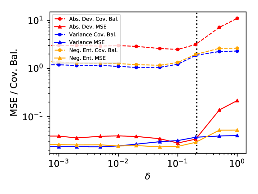
(a) Good overlap, average treatment effect

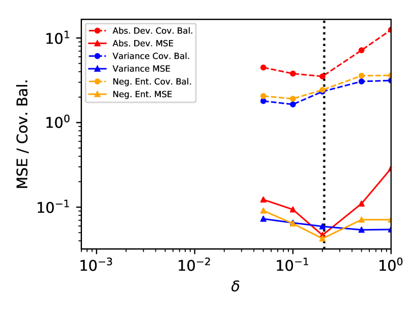
(b) Bad overlap, average treatment effect

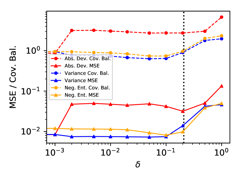
(c) Good overlap, average treatment effect on the treated

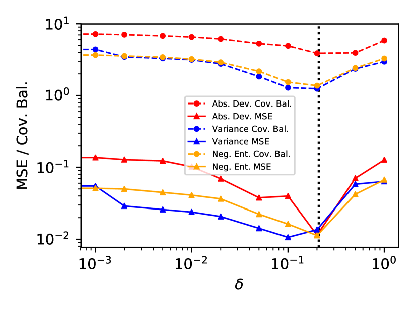
(d) Bad overlap, average treatment effect on the treated

Figure 1: Mean squared error and bootstrapped covariate balance for different values of the tuning parameter $\delta$. In the horizontal axis, $\delta$ starts at 0. The vertical dotted line indicates $\delta=K^{-1/2}$, where $K$ is the number of basis functions balanced. Selecting $\delta$ according to the bootstrapped covariate balance, as in Algorithm 1, often coincides with or neighbors the optimal $\delta$ with the smallest error. We recommend choosing values of $\delta$ smaller than $K^{-1/2}$ as greater values are likely to break the conditions in Assumption 1.

Table 1(a) presents the root mean squared error of minimal weights in estimating the average treatment effect. When the data exhibits bad overlap, minimal weights provide good estimates whereas their exact balancing counterpart does not admit a solution. With good overlap, minimal weights with approximate balancing performs similarly to exact balancing.

Table 1(b) shows the results for the average treatment effect on the treated. In this case, both exact and approximate balance admit solutions under bad overlap. The table shows that approximate balance can markedly reduce the root mean squared error relative to exact balance. We also note that, while we are in a low-dimensional regime (we balance fewer basis functions than the total number of observations), approximate balance (or $\ell_{1}$-regularization) still helps to reduce the error. The reason is that approximate balance trades bias for variance. In fact, when there is bad overlap, traditional weighting estimators that use weights that balance covariates exactly tend to have high variance as they rely heavily on a few observations. In such cases, approximate balance can “pull back” from those observations and trade bias for variance to reduce the overall error.

Figure 1 shows that the root mean squared error of the effect estimates is sensitive to the choice of $\delta$. Moreover, the value of $\delta$ selected by Algorithm 1 often coincides with the optimal value of $\delta$ that produces the lowest mean squared error (solid lines in Figure 1). Again, Algorithm 1 selects the value of $\delta$ that minimizes the bootstrapped covariate balance (dashed lines in Figure 1). We observe that when $\delta$ achieves the lowest bootstrapped covariate balance (dashed lines) it also reaches the lowest error (solid lines). In the figure, the dotted line indicates a value of $\delta$ equal to $K^{-1/2}$, where $K$ is the number of basis functions of the covariates being balanced. We recommend choosing values of $\delta$ smaller than $K^{-1/2}$ for Assumption 1.7 required by Theorem 3 to hold.

In general, minimal weights tuned with Algorithm 1 exhibit better empirical performance in the right heart catheterization data set than their exact balancing counterparts. Empirical studies with the Kang and Schafer (2007) example, the LaLonde (1986) data set, and the Wong and Chan (2018) simulation exhibit a similar pattern. See Appendix D for details.

5 Summary and remarks

Minimal dispersion approximately balancing weights, abbreviated as minimal weights, are the weights of minimal dispersion that approximately balance covariates. In this paper, we study the class of minimal weights from theoretical and practical standpoints. From a theoretical standpoint, we show that under standard technical assumptions minimal weights are consistent estimates of the true inverse probability weights. Also, we show that the resulting minimal weights linear estimator is consistent, asymptotically normal, and semiparametrically efficient. From a practical standpoint, we derive an oracle inequality that bounds the loss incurred by balancing too many functions of the covariates in finite samples. Also, we propose a tuning algorithm to select the degree of approximate balance in minimal weights, which can be of independent interest. Finally, we show that approximate balance is preferable to exact balance in empirical studies, especially when there is limited overlap in covariate distributions.

The theoretical results developed in this work can be extended to matching, where covariates are balanced approximately but with weights that encode an assignment between matched units (e.g., Rubin 1973; Rosenbaum 1989; Hansen 2004; Abadie and Imbens 2006; Zubizarreta 2012; Diamond and Sekhon 2013). The tuning algorithm used to select the degree of approximate balance can also be extended to matching. Promising directions for future work include doubly robust estimation (Robins and Rotnitzky, 1995) where propensity score modeling weights can be substituted by minimal weights (see Athey et al. (2018) and Hirshberg and Wager (2018)). Also, minimal weights can be extended to instrumental variables and regression discontinuity settings where model-based inverse probability weights are used for covariate adjustments.

Supplementary materials

Appendix A Proof for the unconstrained dual formulation

Proof of Theorem 1

Proof.

We first present a vanilla form of the dual.

Lemma 1.

The dual of the optimization problem (1) is

$$\underset{\lambda}{\text{minimize}} l(\lambda)$$

subject to $$\lambda\geq 0$$

where

$$l(\lambda)=\frac{1}{n}\sum^{n}_{j=1}\{-Z_{j}n\rho(Q_{j}^{\top}\lambda)+Q_{j}^{\top}\lambda\}+\lambda^{\top}d,$$

$$A_{K\times n} =\left(\begin{array}[]{cccc}B_{1}(X_{1})&B_{1}(X_{2})&\ldots&B_{1}(X_{n})\\ \vdots&\vdots&\vdots&\vdots\\ B_{K}(X_{1})&B_{K}(X_{2})&\ldots&B_{K}(X_{n})\\ \end{array}\right)_{K\times n},$$

$$Q_{2K\times n}=\left(\begin{array}[]{r}A_{K\times n}\\ -A_{K\times n}\\ \end{array}\right)_{2K\times n},$$

and

$$d_{2K\times 1}=\left(\begin{array}[]{r}\delta_{K\times 1}\\ \delta_{K\times 1}\\ \end{array}\right)_{2K\times 1}.$$

We prove this lemma towards the end of this section.

We then write $\lambda_{2K\times 1}=\left(\begin{array}[]{r}\lambda_{+,K\times 1}\\ \lambda_{-,K\times 1}\\ \end{array}\right)_{2K\times 1}$. We have

$$l(\lambda) =\frac{1}{n}\sum^{n}_{j=1}\{-Z_{j}n\rho(A_{j}^{\top}\lambda_{+}-A_{j}^{\top}\lambda_{-})+(A_{j}^{\top}\lambda_{+}-A_{j}^{\top}\lambda_{-})\}+\lambda_{+}^{\top}\delta+\lambda_{-}^{\top}\delta$$

$$=\frac{1}{n}\sum^{n}_{j=1}[-Z_{j}n\rho\{A_{j}^{\top}(\lambda_{+}-\lambda_{-})\}+A_{j}^{\top}(\lambda_{+}-\lambda_{-})]+(\lambda_{+}^{\top}+\lambda_{-}^{\top})\delta.$$

Suppose the optimizer is $\lambda^{\dagger}_{2K\times 1}=\left(\begin{array}[]{r}\lambda^{\dagger}_{+,K\times 1}\\ \lambda^{\dagger}_{-,K\times 1}\\ \end{array}\right)_{2K\times 1}$. We claim that $\lambda^{\dagger}_{+,k}\cdot\lambda^{\dagger}_{-,k}=0,k=1,\ldots,K$, where the index $k$ points to the $k$th entry of a vector.

We prove this claim by contradiction. Suppose the opposite. If $\lambda^{\dagger}_{+,k}>0$ and $\lambda^{\dagger}_{-,k}>0$ for some $k$, then

$$\lambda^{\dagger\dagger\top}=[\lambda^{\dagger}_{+}-\{0,\ldots,0,\min(\lambda^{\dagger}_{+,k},\lambda^{\dagger}_{-,k}),0,\ldots,0\},\lambda^{\dagger}_{-}-\{0,\ldots,0,\min(\lambda^{\dagger}_{+,k},\lambda^{\dagger}_{-,k}),0,\ldots,0)\}]$$

has

$$l(\lambda^{\dagger\dagger})=l(\lambda^{\dagger})-2\min(\lambda^{\dagger}_{+,k},\lambda^{\dagger}_{-,k})\cdot\delta<l(\lambda^{\dagger})$$

by $\delta>0$ and $\min(\lambda^{\dagger}_{+,k},\lambda^{\dagger}_{-,k})>0$. This contradicts the fact that $\lambda^{\dagger}$ is the optimizer. Theorem 1 then follows by rewriting $\lambda_{+}-\lambda_{-}$ as $\lambda$ and deducing $\lambda_{+}+\lambda_{-}=|\lambda|$ from $\lambda^{\dagger}_{+,k}\cdot\lambda^{\dagger}_{-,k}=0,k=1,\ldots,K$. ∎

Proof of Lemma 1

Proof.

Rewriting problem (1) in matrix notation,

$$\underset{\bm{w}}{\text{minimize}} \sum^{n}_{i=1}Z_{i}h(s_{i})$$

subject to $$Q_{2K\times n}s_{n\times 1}\leq d_{2K\times 1}$$

where

$$s_{n\times 1} =(s_{i})_{n\times 1}=(\frac{1}{n}-Z_{i}w_{i})_{n\times 1},$$

$$A_{K\times n} =\left(\begin{array}[]{cccc}B_{1}(X_{1})&B_{1}(X_{2})&\ldots&B_{1}(X_{n})\\ \vdots&\vdots&\vdots&\vdots\\ B_{K}(X_{1})&B_{K}(X_{2})&\ldots&B_{K}(X_{n})\\ \end{array}\right)_{K\times n},Q_{2K\times n} =\left(\begin{array}[]{r}A_{K\times n}\\ -A_{K\times n}\\ \end{array}\right)_{2K\times n},$$

$$d_{2K\times 1} =\left(\begin{array}[]{r}\delta_{K\times 1}\\ \delta_{K\times 1}\\ \end{array}\right)_{2K\times 1}.$$

Again as special cases, stable balancing weights have $h(x)=(\frac{1}{n}-\frac{1}{r}-x)^{2}$ and entropy balancing has $h(x)=(\frac{1}{n}-x)\log(\frac{1}{n}-x)$.

The problem is now in the form of Tseng and Bertsekas (1987) and Tseng and Bertsekas (1991).

The dual of this problem is

$$\underset{\lambda}{\text{maximize}} g(\lambda)$$

subject to $$\lambda\geq 0,$$

where $g(\lambda)=-\sum^{n}_{j=1}h^{*}_{j}(Q_{j}^{\top}\lambda)-<\lambda,d>,$ and $h_{j}^{*}(\cdot)$ is the convex conjugate of $Z_{j}h(\cdot).$

$$h^{*}_{j}(t) =\sup_{s_{j}}\{ts_{j}-Z_{j}h(s_{j})\}$$

$$=\sup_{w_{j}}\{-tZ_{j}w_{j}+\frac{t}{n}-Z_{j}h(\frac{1}{n}-Z_{j}w_{j})\}$$

$$=\sup_{w_{j}}\{-tZ_{j}w_{j}+\frac{t}{n}-Z_{j}h(\frac{1}{n}-w_{j})\}$$

$$=-tZ_{j}w^{*}_{j}+\frac{t}{n}-Z_{j}h(\frac{1}{n}-w^{*}_{j}),$$

where $w^{*}_{j}$ satisfies the first order condition

$$-tZ_{j}+Z_{j}h^{\prime}(\frac{1}{n}-w^{*}_{j})=0,$$

$$\Rightarrow h^{\prime}(\frac{1}{n}-w^{*}_{j})=t,$$

$$\Rightarrow w^{*}_{j}=\frac{1}{n}-(h^{\prime})^{-1}(t).$$

Therefore,

$$h^{*}_{j}(t) =-tZ_{j}\frac{1}{n}+tZ_{j}(h^{\prime})^{-1}(t)+\frac{t}{n}-Z_{j}h\{(h^{\prime})^{-1}(t)\},$$

$$=-Z_{j}[\frac{t}{n}-t(h^{\prime})^{-1}(t)+h\{(h^{\prime})^{-1}(t)\}]+\frac{t}{n}.$$

Denote $\rho(\cdot)$ as

$$\rho(t)=\frac{t}{n}-t(h^{\prime})^{-1}(t)+h\{(h^{\prime})^{-1}(t)\}.$$

This gives

$$h^{*}_{j}(t)=-Z_{j}\rho(t)+\frac{t}{n}.$$

Also we notice that

$$\rho^{\prime}(t) =\frac{1}{n}-(h^{\prime})^{-1}(t)-t\{(h^{\prime})^{-1}(t)\}^{\prime}+h^{\prime}\{(h^{\prime})^{-1}(t)\}\cdot\{(h^{\prime})^{-1}(t)\}^{\prime}$$

$$=\frac{1}{n}-(h^{\prime})^{-1}(t)-t\{(h^{\prime})^{-1}(t)\}^{\prime}+t\{(h^{\prime})^{-1}(t)\}^{\prime}$$

$$=\frac{1}{n}-(h^{\prime})^{-1}(t).$$

This implies

$$w^{*}=\rho^{\prime}(t).$$

The dual formulation thus becomes

$$\underset{\lambda}{\text{minimize}} l(\lambda)$$

subject to $$\lambda\geq 0$$

where

$$l(\lambda)=\frac{1}{n}\sum^{n}_{j=1}\{-Z_{j}n\rho(Q_{j}^{\top}\lambda)+Q_{j}^{\top}\lambda\}+\lambda^{\top}d.$$

∎

Appendix B Proof of the Asymptotic properties

Proof of Theorem 2

Proof.

The proof utilizes the Bernstein’s inequality as in Fan et al. (2016).

We first prove the following lemma.

Lemma 2.

There exists a global minimizer $\lambda^{\dagger}$ such that

$$||\lambda^{\dagger}-\lambda^{*}_{1}||_{2}=O_{p}(K^{1/2}(\log K)/n+K^{1/2-r_{\pi}}).$$

Proof.

Write $A_{j}=B(X_{j})=\{B_{1}(X_{j}),...,B_{K}(X_{j})\}$. Recall that the optimization objective is

$$G(\lambda):=\frac{1}{n}\sum^{n}_{j=1}\{-Z_{j}n\rho(A_{j}^{\top}\lambda)+A_{j}^{\top}\lambda\}+|\lambda|^{\top}\delta,$$

where $G(\cdot)$ is convex in $\lambda$ by the concavity of $\rho(\cdot).$ To show that a minimizer $\Delta^{*}$ of $G(\lambda^{*}_{1}+\Delta)$ exists in $\mathcal{C}=\{\Delta\in\mathbb{R}^{K}:||\Delta||_{2}\leq CK^{1/2}(\log K)/n+K^{1/2-r_{\pi}}\}$ for some constant $C$, it suffices to show that

$$E\{\inf_{\Delta\in\mathcal{C}}G(\lambda^{*}_{1}+\Delta)-G(\lambda^{*}_{1})>0\}\rightarrow 1,\text{ as }n\rightarrow\infty,(*)$$

by the continuity of $G(\cdot).$

To show $(*)$, we use mean value theorem: for some $\tilde{\lambda}$ between $\lambda^{\dagger}$ and $\lambda_{1}^{*}$,

$$G(\lambda^{*}_{1}+\Delta)-G(\lambda^{*}_{1})$$

$$\geq \Delta\cdot\frac{1}{n}\sum^{n}_{j=1}\{-Z_{j}n\rho^{\prime}(A_{j}^{\top}\lambda^{*}_{1})A_{j}+A_{j}\}+\frac{1}{2}\Delta^{\top}\cdot\{\sum^{n}_{j=1}-Z_{j}\rho^{\prime\prime}(A_{j}^{\top}\tilde{\lambda})A_{j}^{\top}A_{j}\}\cdot\Delta-|\Delta|^{\top}\delta$$

$$\geq -||\Delta||_{2}\cdot||\frac{1}{n}\sum^{n}_{j=1}-Z_{j}n\rho^{\prime}(A_{j}^{\top}\lambda^{*}_{1})A_{j}+A_{j}||_{2}$$

$$+\frac{1}{2}\Delta^{\top}\cdot\{\sum^{n}_{j=1}-Z_{j}\rho^{\prime\prime}(A_{j}^{\top}\tilde{\lambda})A_{j}^{\top}A_{j}\}\cdot\Delta-||\Delta||_{2}||\delta||_{2}$$

$$\geq -||\Delta||_{2}\cdot||\frac{1}{n}\sum^{n}_{j=1}-Z_{j}n\rho^{\prime}(A_{j}^{\top}\lambda^{*}_{1})A_{j}+A_{j}||_{2}-||\Delta||_{2}||\delta||_{2}.$$

The first inequality is due to the triangle inequality, $|\lambda_{1}^{*}+\Delta|-|\lambda_{1}^{*}|\geq-|\Delta|$. The second inequality follows from Cauchy-Schwarz inequality. The third inequality is due to the positivity of $\frac{1}{2}\Delta^{\top}\cdot\{\sum^{n}_{j=1}-Z_{j}\rho^{\prime\prime}(A_{j}^{\top}\tilde{\lambda})A_{j}^{\top}A_{j}\}\cdot\Delta$ by Assumption 1.3.

Next we notice that

$$||\frac{1}{n}\sum^{n}_{j=1}\{-Z_{j}n\rho^{\prime}(A_{j}^{\top}\lambda^{*}_{1})A_{j}+A_{j}\}||_{2}$$

$$\leq ||\frac{1}{n}\sum^{n}_{j=1}(-Z_{j}\frac{1}{\pi_{j}}A_{j}+A_{j})||_{2}+||\frac{1}{n}\sum^{n}_{j=1}-Z_{j}\{\frac{1}{\pi_{j}}-n\rho^{\prime}(A_{j}^{\top}\lambda^{*}_{1})\}A_{j}||_{2}$$

$$\leq ||\frac{1}{n}\sum^{n}_{j=1}(1-\frac{Z_{j}}{\pi_{j}})A_{j}||_{2}+\frac{1}{n}\sum_{j=1}^{n}||A_{j}||_{2}O(K^{-r_{\pi}}).$$

The first inequality is due to the triangle inequality. The second inequality is due to Assumption 1.3 and 1.6.

We first use the Bernstein’s inequality to bound both terms.

Recall that the Bernstein’s inequality for random matrices in Tropp et al. (2015) says the following. Let $\{Z_{k}\}$ be a sequence of independent random matrices with dimensions $d_{1}\times d_{2}$. Assume that $EZ_{k}=0$ and $||Z_{k}||_{2}\leq R_{n}$ almost surely. Define

$$\sigma_{n}^{2}=\max\{||\sum^{n}_{k=1}E(Z_{k}Z_{k}^{\top})||_{2},||\sum^{n}_{k=1}E(Z_{k}^{\top}Z_{k})||_{2}\}.$$

Then for all $t\geq 0$,

$$pr(||\sum^{n}_{k=1}Z_{k}||_{2}\geq t)\leq(d_{1}+d_{2})\exp(-\frac{t^{2}/2}{\sigma^{2}_{n}+R_{n}t/3}).$$

For the first term $||\frac{1}{n}\sum^{n}_{j=1}(1-\frac{Z_{j}}{\pi_{j}})A_{j}||_{2}$, we notice that

$$E\{\frac{1}{n}(1-\frac{Z_{j}}{\pi_{j}})A_{j}\}=E[E\{\frac{1}{n}(1-\frac{Z_{j}}{\pi_{j}})A_{j}\mid X_{j}\}]=0.$$ (5)

The last equality is because $E(Z_{j})=\pi_{j}.$

Then for $||\frac{1}{n}\sum^{n}_{j=1}(1-Z_{j}/\pi_{j})A_{j}||_{2}$, we have

$$||\frac{1}{n}(1-\frac{Z_{j}}{\pi_{j}})A_{j}||_{2}$$

$$\leq \frac{1}{n}||(1-\frac{Z_{j}}{\pi_{j}})||_{2}||A_{j}||_{2}$$

$$\leq \frac{1}{n}(\frac{1-\pi_{j}}{\pi_{j}})CK^{1/2}$$

$$= \frac{1}{n}\{n\rho^{\prime}(A_{j}^{\top}\lambda_{1}^{*})-1\}CK^{1/2}$$

$$\leq C^{\prime}\frac{K^{1/2}}{n}.$$ (6)

The first inequality is due to Cauchy-Schwarz inequality. The second inequality is due to Assumption 1.4 and $E(1-Z_{j}/\pi_{j})^{2}=\text{var}(1-Z_{j}/\pi_{j})=\pi_{j}(1-\pi_{j})/\pi_{j}^{2}=(1-\pi_{j})/\pi_{j}$. The third equality is due to $\pi_{j}=\{n\rho^{\prime}(A_{j}^{\top}\lambda_{1}^{*})\}^{-1}.$ The fourth inequality is due to Assumption 1.3.

Finally, for $||\sum^{n}_{k=1}E\{\frac{1}{n^{2}}(1-\frac{Z_{j}}{\pi_{j}})^{2}A_{j}A_{j}^{\top}\}||_{2}$, we have

$$||\sum^{n}_{k=1}E\{\frac{1}{n^{2}}(1-\frac{Z_{j}}{\pi_{j}})^{2}A_{j}A_{j}^{\top}\}||_{2}$$

$$\leq \frac{1}{n}\sup_{j}(1-\frac{Z_{j}}{\pi_{j}})^{2}||E(A_{j}A_{j}^{\top})||_{2}$$

$$\leq \frac{C^{\prime\prime}}{n}.$$ (7)

The first inequality is taking the sup over $(1-\frac{Z_{j}}{\pi_{j}})^{2}$. The second inequality is due to Assumption 1.3, 1.4, and $\pi_{j}=\{n\rho^{\prime}(A_{j}^{\top}\lambda_{1}^{*})\}^{-1}.$

Equation 5, Equation 6, and Equation 7, together with the Bernstein’s inequality, imply

$$\textrm{pr}\{||\frac{1}{n}\sum^{n}_{j=1}(1-\frac{Z_{j}}{\pi_{j}})A_{j}||_{2}\geq t\}\leq(K+1)\exp(-\frac{t^{2}/2}{\frac{C^{\prime\prime}}{n}+C^{\prime}\frac{K^{1/2}}{n}\cdot t/3}).$$

The right side goes to zero as $K\rightarrow\infty$ when

$$\frac{t^{2}/2}{\frac{C^{\prime\prime}}{n}+C^{\prime}\frac{K^{1/2}}{n}\cdot t/3}\geq\log K.$$

It suffices when $t=O_{p}\{K^{1/2}(\log K)/n\}.$

Therefore, we have

$$||\frac{1}{n}\sum^{n}_{j=1}(1-\frac{Z_{j}}{\pi_{j}})A_{j}||_{2}=O_{p}\{K^{1/2}(\log K)/n\}.$$ (8)

Now we work on the second term $\frac{1}{n}\sum_{j=1}^{n}||A_{j}||_{2}O(K^{-r_{\pi}})$. We have

$$\frac{1}{n}\sum_{j=1}^{n}||A_{j}||_{2}O(K^{-r_{\pi}})\leq CK^{1/2-r_{\pi}}.$$ (9)

This inequality is due to Assumption 1.4.

Combining Equation 8, Equation 9, and Assumption 1.7, we have

$$G(\lambda^{*}_{1}+\Delta)-G(\lambda^{*}_{1})$$

$$= -||\Delta||_{2}\cdot O_{p}(\frac{K^{1/2}\log K}{n}+K^{1/2-r_{\pi}})+\frac{1}{2}||\Delta||^{2}_{2}||\delta||_{2}$$

$$\geq 0$$

for $\Delta=C\frac{K^{1/2}\log K}{n}+K^{1/2-r_{\pi}}$ with large enough constant $C>0.$

$(*)$ is thus proved. ∎

Now we prove Theorem 2.

$$\sup_{x\in\mathcal{X}}|nw^{*}(x)-\frac{1}{\pi(x)}|$$

$$= \sup_{x\in\mathcal{X}}|n\rho^{\prime}\{B(x)^{\top}\lambda^{\dagger}\}-n\rho^{\prime}\{m^{*}(x)\}|$$

$$\leq \sup_{x\in\mathcal{X}}|n\rho^{\prime}\{B(x)^{\top}\lambda^{\dagger}\}-n\rho^{\prime}\{B(x)^{\top}\lambda^{*}_{1}\}|+\sup_{x\in\mathcal{X}}|n\rho^{\prime}\{B(x)^{\top}\lambda^{*}_{1}\}-n\rho^{\prime}\{m^{*}(x)\}|$$

$$= O\{\sup_{x\in\mathcal{X}}|B(x)^{\top}\lambda^{\dagger}-B(x)^{\top}\lambda^{*}_{1}|\}+O(K^{-r_{\pi}})$$

$$\leq O\{\sup_{x\in\mathcal{X}}||B(x)||_{2}||\lambda^{\dagger}-\lambda^{*}_{1}||_{2}\}+O(K^{-r_{\pi}})$$

$$= O_{p}\{K(\frac{\log K}{n}+K^{-r_{\pi}})\}+O(K^{-r_{\pi}})$$

$$= O_{p}(\frac{K\log K}{n}+K^{1-r_{\pi}})$$

$$= o_{p}(1)$$

The first equality rewrites $\pi(x)=\{n\rho^{\prime}(B(x)^{\top}\lambda_{1}^{*})\}^{-1}.$ The second inequality is due to the triangle inequality. The third inequality is due to Assumptions 1.3 and 1.6. The fourth inequality is due to the Cauchy-Schwarz inequality. The fifth equality is due to Lemma 2 and Assumption 1.4. The sixth equality holds because the first term dominates the second. The seventh equality is due to Assumptions 1.5 and 1.6.

Also, we have

$$||nw^{*}(x)-\frac{1}{\pi(x)}||_{P,2}$$

$$= ||n\rho^{\prime}\{\lambda^{\dagger\top}B(X)\}-\frac{1}{\pi(x)}||_{P,2}$$

$$\lesssim ||n\rho^{\prime}\{\lambda^{\dagger\top}B(X)\}-n\rho^{\prime}\{\lambda_{1}^{*\top}B(X)\}||_{P,2}+||\frac{1}{\pi(x)}-n\rho^{\prime}\{\lambda_{1}^{*\top}B(X)\}||_{P,2}$$

$$\lesssim ||(\lambda^{\dagger}-\lambda_{1}^{*})^{\top}B(X)||_{P,2}+\sup_{x\in\mathcal{X}}|m^{*}(x)-\lambda_{1}^{*\top}B(x)|$$

$$= O_{p}\{K^{1/2}(\frac{\log K}{n}+K^{-r_{\pi}})\}+O(K^{-r_{\pi}})$$

$$= O_{p}(\frac{K^{1/2}\log K}{n}+K^{1/2-r_{\pi}})$$

$$= o_{p}(1)$$

The first equality rewrites $\pi(x)=[n\rho^{\prime}\{B(x)^{\top}\lambda_{1}^{*}\}]^{-1}.$ The second inequality is due to the triangle inequality. The third inequality is due to Assumption 1.3. The fourth inequality is due to Lemma 2, Assumption 1.4 and Assumption 1.6. The fifth equality is due to the first term dominates the second. The sixth equality is due to Assumption 1.5 and Assumption 1.6.

∎

Proof of Theorem 3

Proof.

The proof utilizes empirical processes techniques as in Fan et al. (2016).

We first decompose $\hat{Y}_{w^{*}}-\bar{Y}$ into several residual terms.

$$\hat{Y}_{w^{*}}-\bar{Y} =\sum^{n}_{i=1}Z_{i}w^{*}_{i}Y_{i}-\bar{Y}$$

$$=\sum^{n}_{i=1}Z_{i}w^{*}_{i}\{Y_{i}-Y(X_{i})\}+\sum^{n}_{i=1}(Z_{i}w^{*}_{i}-\frac{1}{n})Y(X_{i})+\{\frac{1}{n}\sum^{n}_{i=1}Y(X_{i})-\bar{Y}\}$$

$$\begin{split}&=\sum^{n}_{i=1}Z_{i}w^{*}_{i}\{Y_{i}-Y(X_{i})\}+\sum^{n}_{i=1}(Z_{i}w^{*}_{i}-\frac{1}{n})\{Y(X_{i})-\lambda_{2}^{*\top}B(X_{i})\}\\ &+\sum^{n}_{i=1}(Z_{i}w^{*}_{i}-\frac{1}{n})\lambda_{2}^{*\top}B(X_{i})+\{\frac{1}{n}\sum^{n}_{i=1}Y(X_{i})-\bar{Y}\}\end{split}$$

$$=\frac{1}{n}\sum^{n}_{i=1}S_{i}+R_{0}+R_{1}+R_{2},$$

where

$$S_{i} =\frac{Z_{i}}{\pi_{i}}\{Y_{i}-Y(X_{i})\}+\{Y(X_{i})-\bar{Y}\},$$

$$R_{0} =\sum^{n}_{i=1}(w^{*}_{i}-\frac{1}{n\pi_{i}})Z_{i}\{Y_{i}-Y(X_{i})\},$$

$$R_{1} =\sum^{n}_{i=1}(Z_{i}w^{*}_{i}-\frac{1}{n})\{Y(X_{i})-\lambda_{2}^{*\top}B(X_{i})\},$$

$$R_{2} =\sum^{n}_{i=1}(Z_{i}w^{*}_{i}-\frac{1}{n})\{\lambda_{2}^{*\top}B(X_{i})\}.$$

Below we show $R_{j}=o_{p}(n^{-1/2}),0\leq j\leq 2$. The conclusion follows from $S_{i}$ taking the same form as the efficient score (Hahn, 1998). $\hat{Y}_{w^{*}}$ is thus asymptotically normal and semiparametrically efficient.

We first study $R_{0}=\sum^{n}_{i=1}(nw^{*}_{i}-1/\pi_{i})Z_{i}\{Y_{i}-Y(X_{i})\}/n$. Consider an empirical process $\mathbb{G}_{n}(f_{0})=n^{1/2}[\sum^{n}_{i=1}f_{0}(Z_{i},Y_{i},X_{i})/n-E\{f_{0}(Z,Y,X)\}]$, where

$$f_{0}(Z,Y,X)=Z\{Y-Y(X)\}\left[n\rho^{\prime}\{m(X)\}-\frac{1}{\pi(x)}\right].$$

By the missing at random assumption, we have $Ef_{0}\{Z,Y,X\}=0.$

By Theorem 2, we have

$$\sup_{x\in\mathcal{X}}|\rho^{\prime}\{B(x)^{\top}\lambda^{\dagger}\}-\frac{1}{n\pi(x)}|=O_{p}(\frac{K\log K}{n}+K^{1-r_{\pi}})=o_{p}(1).$$

By Markov’s inequality and maximal inequality, we have

$$n^{1/2}R_{0}\leq\sup_{f_{0}\in\mathcal{F}}\mathbb{G}_{n}(f_{0})\lesssim E\sup_{f_{0}\in\mathcal{F}}\mathbb{G}_{n}(f_{0})\lesssim J_{[]}\{||F_{0}||_{P,2},\mathcal{F},L_{2}(P)\},$$

where the set of functions is $\mathcal{F}=\{f_{0}:||m-m^{*}||_{\infty}\leq\delta_{0}\}$, where $||f||_{\infty}=\sup_{x\in\mathcal{X}}|f(x)|$ and $\delta_{0}=C\{K(\log K)/n+K^{1-r_{\pi}}\}$ for some constant $C>0$.

The second inequality is due to Markov’s inequality. $J_{[]}\{||F_{0}||_{P,2},\mathcal{F},L_{2}(P)\}$ is the bracketing integral. $F_{0}:=\delta_{0}|Y-Y(X)|\gtrsim|f_{0}(Z,Y,X)|$ is the envelop function. We also have $||F_{0}||_{P,2}=(EF_{0}^{2})^{1/2}\lesssim\delta_{0}$ by $E|Y-Y(X)|<\infty.$

Next we bound $J_{[]}\{||F_{0}||_{P,2},\mathcal{F},L_{2}(P)\}$ by $n_{[]}\{\varepsilon,\mathcal{F},L_{2}(P)\}$:

$$J_{[]}\{||F_{0}||_{P,2},\mathcal{F},L_{2}(P)\}\lesssim\int^{\delta}_{0}[n_{[]}\{\varepsilon,\mathcal{F},L_{2}(P)\}]^{1/2}\text{d}\varepsilon.$$

Define a new set of functions $\mathcal{F}_{0}=\{f_{0}:||m-m^{*}||_{\infty}\leq C\}$ for some constant $C>0$. Then,

$$\log n_{[]}\{\varepsilon,\mathcal{F},L_{2}(P)\} \lesssim\log n_{[]}\{\varepsilon,\mathcal{F}_{0}\delta_{0},L_{2}(P)\}$$

$$=\log n_{[]}\{\varepsilon/\delta_{0},\mathcal{F}_{0},L_{2}(P)\}$$

$$\lesssim\log n_{[]}\{\varepsilon/\delta_{0},\mathcal{M},L_{2}(P)\}$$

$$\lesssim(\delta_{0}/\varepsilon)^{(1/k_{1})}.$$

The first inequality is due to the fact that $\rho^{\prime}(\cdot)$ bounded away from 0 and Lipschitz. The last inequality is due to Assumption 2.2.

Therefore, we have

$$J_{[]}\{||F_{0}||_{P,2},\mathcal{F},L_{2}(P)\}\lesssim\int^{\delta}_{0}[\log n_{[]}\{\varepsilon,\mathcal{F},L_{2}(P)\}]^{1/2}\text{d}\varepsilon\lesssim\int^{\delta}_{0}(\delta_{0}/\varepsilon)^{(1/2k_{1})}\text{d}\varepsilon.$$

This goes to 0 as $\delta$ goes to 0 by $2k_{1}>1$ and the integral converges. Thus, this shows that $n^{1/2}R_{0}=o_{p}(1)$.

Next, we consider $R_{1}=\sum^{n}_{i=1}(nZ_{i}w^{*}_{i}-1)\{Y(X_{i})-\lambda_{2}^{*\top}B(X_{i})\}/n$. Define the empirical process $\mathbb{G}_{n}(f_{1})=n^{1/2}[\sum^{n}_{i=1}f_{1}(Z_{i},X_{i})/n-E\{f_{1}(Z,X)\}]$, where $f_{1}(Z,X)=[nZ\rho^{\prime}\{m(x)\}-1]\{Y(X)-\lambda_{2}^{*\top}B(X)\}$.

Write $\Delta(X):=Y(X)-\lambda_{2}^{*\top}B(X).$ By Assumption 2.3, we have $||\Delta||_{\infty}\lesssim K^{-r_{y}}$.

By Theorem 2, we have

$$\left\|n\rho^{\prime}\{\lambda^{\dagger\top}B(X)\}-\frac{1}{\pi(x)}\right\|_{P,2}=O_{p}(\frac{K\log K}{n}+K^{1-r_{\pi}}).$$

Therefore, we have

$$n^{1/2}R_{1} =\mathbb{G}_{n}(f_{1})+n^{1/2}Ef_{1}(Z,X)$$

$$\leq\sup_{f_{1}\in\mathcal{F}_{1}}\mathbb{G}_{n}(f_{1})+n^{1/2}\sup_{f_{1}\in\mathcal{F}_{1}}Ef_{1},$$

where $\mathcal{F}_{1}=\{f_{1}:||m-m^{*}||_{P,2}\leq\delta_{1},$$||\Delta||_{\infty}\leq\delta_{2}\},$$\delta_{1}=C\{K^{1/2}(\log K)/n+K^{1/2-r_{\pi}}\}$, $\delta_{2}=CK^{-r_{y}}$ for some constant $C>0.$

Again, by Markov’s inequality and the maximal inequality,

$$\sup_{f_{1}\in\mathcal{F}_{1}}\mathbb{G}_{n}(f_{1})\lesssim E\sup_{f_{1}\in\mathcal{F}_{1}}\mathbb{G}_{n}(f_{1})\lesssim J_{[]}\{||F_{1}||_{P,2},\mathcal{F},L_{2}(P)\},$$

where $F_{1}:=C\delta_{2}$ for some constant $C>0$ so that $||F_{1}||_{P,2}\lesssim\delta_{2}.$

Similar to characterizing $R_{1}$, we we bound $J_{[]}(||F_{1}||_{P,2},\mathcal{F}_{1},L_{2}(P)$ by $n_{[]}(\varepsilon,\mathcal{F}_{1},L_{2}(P))$:

$$J_{[]}(||F_{1}||_{P,2},\mathcal{F}_{1},L_{2}(P)\lesssim\int^{\delta}_{0}\{n_{[]}(\varepsilon,\mathcal{F}_{1},L_{2}(P))\}^{1/2}\text{d}\varepsilon.$$

Then, we bound $n_{[]}(\varepsilon,\mathcal{F}_{1},L_{2}(P))$:

$$\log n_{[]}\{\varepsilon,\mathcal{F}_{1},L_{2}(P)\} \lesssim\log n_{[]}\{\varepsilon/\delta_{2},\mathcal{F}_{0},L_{2}(P)\}$$

$$\lesssim\log n_{[]}\{\varepsilon/\delta_{2},G_{10},L_{2}(P)\}+\log n_{[]}\{\varepsilon/\delta_{2},G_{20},L_{2}(P)\}$$

$$\lesssim\log n_{[]}\{\varepsilon/\delta_{2},\mathcal{M},L_{2}(P)\}+\log n_{[]}\{\varepsilon/\delta_{2},\mathcal{H},L_{2}(P)\}$$

$$\lesssim(\delta_{1}/\varepsilon)^{1/k_{1}}+(\delta_{2}/\varepsilon)^{1/k_{2}}.$$

where

$$\mathcal{F}_{0}=\{f_{1}:||m-m^{*}||_{P,2}\leq C,||\Delta||_{P,2}\leq 1\},$$

$$\mathcal{G}_{10}=\{m\in\mathcal{M}+m^{*}:||m||_{P,2}\leq C\},$$

$$\mathcal{G}_{20}=\{\Delta\in\mathcal{H}-\lambda_{2}^{*\top}B(x):||\Delta||_{P,2}\leq 1\}.$$

The second inequality is due to $\rho^{\prime}$ is Lipschitz and bounded away from 0.

Therefore we have

$$J_{[]}\{||F_{1}||_{P,2},\mathcal{F}_{1},L_{2}(P)\}\lesssim\int^{\delta}_{0}(\delta_{1}/\varepsilon)^{(1/2k_{1})}d\varepsilon+\int^{\delta}_{0}(\delta_{2}/\varepsilon)^{(1/2k_{2})}d\varepsilon.$$

By $2k_{1}>1$ and $2k_{2}>1$, we have $J_{[]}\{||f_{1}||_{P,2},\mathcal{F},L_{2}(P)\}=o(1)$. This gives $\sup_{f_{1}\in\mathcal{F}_{1}}\mathbb{G}_{n}(f_{1})=o_{p}(1)$.

Now we look at $n^{1/2}\sup_{f_{1}\in\mathcal{F}_{1}}Ef_{1},$

$$n^{1/2}\sup_{f_{1}\in\mathcal{F}}Ef_{1} =n^{1/2}\sup_{m\in\mathcal{G}_{1},\Delta\in\mathcal{G}_{2}}E\{\pi(X)[n\rho^{\prime}\{m(X)\}-1]\Delta(X)\}$$

$$=n^{1/2}\sup_{m\in\mathcal{G}_{1},\Delta\in\mathcal{G}_{2}}E([n\rho^{\prime}\{m(x)\}-\frac{1}{\pi(x)}]\pi(x)\Delta(x))$$

$$\lesssim n^{1/2}\sup_{m\in\mathcal{G}_{1}}||n\rho^{\prime}\{m(x)\}-\frac{1}{\pi(x)}||_{P,2}\sup_{\Delta\in\mathcal{G}_{2}}||\Delta(x)||_{P,2}$$

$$\lesssim n^{1/2}\delta_{1}\delta_{2}=o_{p}(1),$$

where $\mathcal{G}_{1}=\{m\in\mathcal{M}:||m-m^{*}||_{P,2}\leq\delta_{1}\},\mathcal{G}_{2}=\{\Delta\in\mathcal{H}-\lambda_{2}^{*\top}B(x):||\Delta||_{\infty}\leq\delta_{2}\}$.

The last equality is due to the assumption $n^{1/2}\lesssim K^{r_{\pi}+r_{y}-1/2}$.

Therefore, we can conclude that $n^{1/2}R_{1}=o_{p}(1).$

Lastly, $R_{2}=\lambda_{2}^{*\top}\{\sum^{n}_{i=1}(Z_{i}w^{*}_{i}-1/n)B(X_{i})\}=o_{p}(1)$ by $\sum^{n}_{i=1}(Z_{i}w^{*}_{i}-1/n)B(X_{i})\leq||\delta||^{2}=o_{p}(1)$ due to the constraints posited in the optimization problem for minimal weights.

We finally prove the consistency of the variance estimator. We need a stronger smoothness assumption, i.e. $r_{y}>1$.

Under assumptions 1 and 2, we construct a variance estimator based on a direct approximation of the efficient influence function. Recall that the efficient influence function determines the semiparametric efficiency bound (Hahn, 1998):

$$V_{opt} :=var(Y(X_{i}))+E\{var(Y|X_{i})/\pi(X_{i})\}$$

$$=E\left\{\left(\frac{Z_{i}Y_{i}}{\pi(X_{i})}-\bar{Y}-Y(X_{i})(\frac{Z_{i}}{\pi(X_{i})}-1)\right)^{2}\right\}.$$

We estimate $V_{opt}$ with $\hat{V}_{K}$:

$$\begin{split}\hat{V}_{K}=&\frac{1}{n}\sum^{n}_{i=1}\left[nZ_{i}w_{i}Y_{i}-\sum_{i=1}^{n}w_{i}Y_{i}\right.\\ &\left.-B(X_{i})^{\top}\left\{\frac{1}{n}\sum_{i=1}^{n}Z_{i}w_{i}B(X_{i})^{\top}B(X_{i})\right\}^{-1}\right.\left.\left\{\frac{1}{n}\sum_{i=1}^{n}Z_{i}w_{i}B(X_{i})^{\top}Y_{i}\right\}(nZ_{i}w_{i}-1)\right]^{2}.\end{split}$$

In particular, $\{\frac{1}{n}\sum_{i=1}^{n}Z_{i}w_{i}B(X_{i})^{\top}B(X_{i})\}^{-1}\{\frac{1}{n}\sum_{i=1}^{n}Z_{i}w_{i}B(X_{i})^{\top}Y_{i}\}$ is a least square estimator of $Y(X_{i})$.

To show $\hat{V}_{K}$ is consistent with $V_{opt}$, it is sufficient to show

$$|B(X_{i})^{\top}\{\frac{1}{n}\sum_{i=1}^{n}Z_{i}w_{i}B(X_{i})^{\top}B(X_{i})\}^{-1}\{\frac{1}{n}\sum_{i=1}^{n}Z_{i}w_{i}B(X_{i})^{\top}Y_{i}\}-Y(X_{i})|\stackrel{{\scriptstyle a.s.}}{{\rightarrow}}0.\qquad(**)$$

This is because $nw_{i}$ is a consistent estimator of $1/\pi(X_{i})$ by Theorem 2 and $\sum_{i=1}^{n}w_{i}Y_{i}$ is a consistent estimator of $\bar{Y}$ by Theorem 3.

Below we prove $(**)$.

We first rewrite $Y_{i}$ as $Y_{i}=B(X_{i})^{\top}\lambda_{2}^{*}+\gamma+\epsilon_{i},$ where $\gamma=O(K^{-r_{y}})$ from Assumption 2.3, and $\epsilon_{i}$ is some iid zero mean error with variance $\sigma^{2}=var(Y|X_{i})$. Therefore,

$$\{\frac{1}{n}\sum_{i=1}^{n}Z_{i}w_{i}B(X_{i})^{\top}B(X_{i})\}^{-1}\{\frac{1}{n}\sum_{i=1}^{n}Z_{i}w_{i}B(X_{i})^{\top}Y_{i}\}$$

$$= \{\frac{1}{n}\sum_{i=1}^{n}Z_{i}w_{i}B(X_{i})^{\top}B(X_{i})\}^{-1}[\frac{1}{n}\sum_{i=1}^{n}Z_{i}w_{i}B(X_{i})^{\top}\{B(X_{i})^{\top}\lambda_{2}^{*}+\gamma+\epsilon_{i}\}]$$

$$= \lambda^{*}_{2}+\{\frac{1}{n}\sum_{i=1}^{n}Z_{i}w_{i}B(X_{i})^{\top}B(X_{i})\}^{-1}\{\frac{1}{n}\sum_{i=1}^{n}Z_{i}w_{i}B(X_{i})^{\top}\}\gamma$$

$$+\{\frac{1}{n}\sum_{i=1}^{n}Z_{i}w_{i}B(X_{i})^{\top}B(X_{i})\}^{-1}\{\frac{1}{n}\sum_{i=1}^{n}Z_{i}w_{i}B(X_{i})^{\top}\epsilon_{i}\}$$

$$= \lambda^{*}_{2}+E\{Z_{i}w_{i}B(X_{i})^{\top}B(X_{i})\}^{-1}E\{Z_{i}w_{i}B(X_{i})^{\top}\}\{\gamma+E(\epsilon_{i})\}+O_{p}(n^{-1/2})$$

$$= \lambda^{*}_{2}+O_{p}(K^{-r_{y}+1/2}).$$

The last equality is due to assumptions 1.4 and 2.3 and the law of large numbers.

Finally we have

$$B(X_{i})^{\top}\{\frac{1}{n}\sum_{i=1}^{n}Z_{i}w_{i}B(X_{i})^{\top}B(X_{i})\}^{-1}\{\frac{1}{n}\sum_{i=1}^{n}Z_{i}w_{i}B(X_{i})^{\top}Y_{i}\}$$

$$= B(X_{i})^{\top}\lambda^{*}_{2}+B(X_{i})\cdot O_{p}(K^{-r_{y}+1/2})$$

$$= Y(X_{i})+B(X_{i})\cdot O_{p}(K^{-r_{y}+1/2})+O_{p}(K^{-r_{y}})$$

$$= Y(X_{i})+o_{p}(1)$$

The last equality is due to assumption 1.4 and the additional assumption $r_{y}>1$. ∎

Appendix C Theorem 4 explained

Due to the connection to shrinkage estimation, for each basis function that we balance, we implicitly include a corresponding term in the inverse propensity score model. In practice, we are often concerned about the estimation loss due to fitting an overly complex model. In the context of minimal weights, an overly complex model corresponds to balancing more terms than are needed.

Theorem 4 is an oracle inequality that bounds this loss and states that approximate balancing—as opposed to exact balancing—mimics the act of upper bounding the number of effective balancing constraints. Hence, minimal weights do not suffer much from excessive balancing when few constraints are active. We also remark that this sparsity assumption on the balancing constraints is commonly satisfied in real data sets. This is exemplified by the sparsity of the shadow prices in the 2010 Chilean post earthquake survey data; see Figure 1 of Zubizarreta (2015).

The oracle inequality we proved in Section 4 leverages an oracle inequality for lasso in the high dimensional generalized linear model literature (Van de Geer, 2008). The original oracle inequality says the lasso estimator (with $\ell^{1}$ penalty) under general Lipschitz losses behaves similarly to the estimator with $\ell^{0}$ penalty, if the true generalized linear model is sparse.

Recall that the minimal weights compute

$$\lambda^{\dagger}:=\operatorname*{arg\,min}G(\lambda)=\operatorname*{arg\,min}\sum^{n}_{j=1}\left\{-Z_{j}\rho(A_{j}^{\top}\lambda)+A_{j}^{\top}\lambda\cdot\frac{1}{n}\right\}+|\lambda|^{\top}\delta.$$

This is a lasso estimator under the loss function

$$L_{w}(x,z)=-z\cdot n(\rho\circ(\rho^{\prime})^{-1}\circ w)(x)+((\rho^{\prime})^{-1}\circ w)(x),$$

where the fit for $w$ is $\hat{w}(x)=\rho^{\prime}(B(x)^{\top}\hat{\lambda})$. This loss function is the same loss function as in Equation 4 but written as a function of $w$. Correspondingly, the empirical loss is

$$\sum_{n}^{i=1}L_{w}(X_{i},Z_{i})=\frac{1}{n}\sum^{n}_{i=1}\left\{-Z_{i}n\cdot(\rho\circ(\rho^{\prime})^{-1}\circ w)(X_{i})+((\rho^{\prime})^{-1}\circ w)(X_{i})\right\},$$

and the theoretical risk is

$$EL_{w}(X,Z)= \frac{1}{n}\sum^{n}_{i=1}E\left\{-Z_{i}n\cdot(\rho\circ(\rho^{\prime})^{-1}\circ w)(X_{i})+((\rho^{\prime})^{-1}\circ w)(X_{i})\right\}$$

$$= \frac{1}{n}\sum^{n}_{i=1}\left\{-\pi(X_{i})\cdot n(\rho\circ(\rho^{\prime})^{-1}\circ w)(X_{i})+((\rho^{\prime})^{-1}\circ w)(X_{i})\right\}.$$

We define the target $w^{0}$ as the minimizer of the theoretical risk

$$w^{0}(x):=\operatorname*{arg\,min}EL_{w}(X,Z)=\frac{1}{n\pi(x)}.$$

The last equality is due to setting $\partial EL_{w}(X,Z)/\partial w=0.$ This is the true inverse propensity score function used for inverse probability weights. We are interested in studying the excess risk of estimators

$$\mathcal{E}(w):=E\{L_{w}(X,Z)-L_{w^{0}}(X,Z)\}.$$

For simplicity of notation, we write $w_{\lambda}(x)=\rho^{\prime}(B(x)^{\top}\lambda),\lambda\in\mathbb{R}^{K}$. Approximate balancing weights thus perform the empirical risk minimization of

$$\lambda^{\dagger}:=\operatorname*{arg\,min}_{\lambda}\{\frac{1}{n}\sum^{n}_{i=1}L_{w_{\lambda}}(X_{i},Z_{i})+|\lambda|^{\top}\delta\}.$$

We look at the case of $\delta=\delta^{+}(\hat{\sigma}_{1},\hat{\sigma}_{2},...,\hat{\sigma}_{K}),$ for some $\delta^{+}>0$, where $\hat{\sigma}_{k}$ is the (sample) standard error of $B_{k}(X),k=1,...,K$. This aligns closely with the common way of setting $\delta$; we specify approximate balancing constraints in units of the standard error of each covariate.

We consider the following oracle estimator

$$\lambda^{*}:=\operatorname*{arg\,min}_{\lambda}\{EL_{w_{\lambda}}(X,Z)+||\lambda||_{0}\cdot C_{0}\},$$

for some constant $C_{0}>0.$ $\lambda^{*}$ can also be seen as the minimizer of $\mathbb{P}L_{w_{\lambda}}$ under the constraint that $||\lambda||_{0}\leq C_{1}$ for some $C_{1}>0$.

$||\lambda||_{0}$ is the number of nonzero entries of $\lambda.$ This is also the number of active or effective covariate balancing constraints in the optimization problem (1). In this sense, the oracle estimator roughly performs the same covariate balancing exactly as its approximate counterpart $\lambda^{\dagger}$ but the number of effective constraints being capped by some constant.

We now assume the following conditions hold and present the oracle inequality.

Assumption 3.

The following conditions hold:

1. There exist constants $0<c_{0}<1/2,$ such that $c_{0}\leq n\rho^{\prime}(v)\leq 1-c_{0}$ for any $v=B(x)^{\top}\lambda$ with $\lambda\in int(\Theta)$. Also, there exist constants $c_{1}<c_{2}<0$, such that $c_{1}\leq n\rho^{\prime\prime}(v)\leq c_{2}<0$ in some small neighborhood $\mathcal{B}$ of $v^{*}=B(x)^{\top}\lambda^{\dagger}$.

2. $\epsilon_{0}<\pi(x)<1-\epsilon_{0},\forall x$, for some constant $0<\epsilon_{0}<1$,

3. $M:=\max||B_{k}(x)||_{\infty}/\sigma_{k}<\infty,$ where $\sigma_{k}$ is the (population) standard deviation of $B_{k}(X),k=1,...,K.$

Commenting on the previous assumptions, Assumption 3.1 is similar to Assumption 1.3. Assumption 3.2 is similar to the overlap condition of propensity scores. Both of them ensure the quadratic margin condition required by the lasso oracle inequality (the quadratic margin condition says in the $\ell^{\infty}$ neighborhood of $w^{0}$ the excess risk $\mathcal{E}$ is bounded from below by a quadratic function). Assumption 3.3 is similar to Assumption 1.4. It ensures the existence of the constant $\bar{\lambda}>0$ in the theorem.

We further assume the following technical conditions.

Assumption 4.

Assume the following technical conditions hold.

1. There exists $\eta>0$ such that $n||w_{\lambda^{*}}-w^{0}||_{\infty}\leq\eta$ and $n||w_{\tilde{\lambda}-w^{0}}||_{\infty}\leq\eta$, where $\tilde{\lambda}=\operatorname*{arg\,min}_{\lambda\in\Theta:\sum_{k}\sigma_{k}|\lambda-\lambda^{*}|\leq 9\mathcal{E}(w_{\lambda^{*}})+675\bar{\lambda^{2}}||\lambda^{*}||_{0}}\{\mathcal{E}(w_{\lambda})-15\bar{\lambda}\sum_{k:\lambda^{*}\neq 0}\sigma_{k}|\lambda-\lambda^{*}|\}$,

2. $\{\log(2K)\}^{1/2}n^{-1/2}M\leq 0.13,$

3. $a_{n}:=\{2\log(2K)\}^{1/2}Mn^{-1/2}+\log(2K)Mn^{-1/2},$

4. For some $t>0$ we are free to set, $\bar{\lambda}:=4a_{n}(1+t\{2(1+8a_{n}M)\}^{1/2}+8t^{2}a_{n}M/3)>6.4\{\log(2K)\}^{1/2}n^{-1/2},$

5. $s>0$ solves $a_{n}(1+s\{2(1+2a_{n}M)\}^{1/2}+2t^{2}a_{n}M/3)=9/5,$

6. $\alpha=\exp(-na_{n}^{2}s^{2})+7\exp(-4na_{n}t^{2}).$

The technical assumptions are inherited from Theorem 2.2 of Van de Geer (2008).

The first technical assumption is needed because the quadratic margin condition $\mathcal{E}(nw_{\lambda})\geq cn||w_{\lambda}-w^{0}||^{2}$ only holds locally for $w_{\eta}$ within the $\eta$ neighborhood of $w^{0}$, $||w_{\lambda}-w^{0}||_{\infty}\leq\eta/n.$ The estimator $\tilde{\lambda}$ strikes the balance between how much excess risk it incurs and how different it is from the oracle estimator $\lambda^{*}$ in the $\ell^{1}$ neighborhood of $\lambda^{*}$.

The second technical assumption is to ensure the applicability of Bousquet’s inequality to the empirical process induced by $Z$ conditional on $X$. The constant 0.13 is rather arbitrary; it could be replaced by any constant smaller that $(\sqrt{6}-\sqrt{2})/2$ if other constants are adjusted accordingly.

The third technical assumption on $a_{n}$ is due to the usual rate of decay in probability for Gaussian linear model with orthogonal design, resulting from a symmetrization inequality and a contraction inequality.

The fourth technical assumption on $\bar{\lambda}$ is setting a lower bound for the smoothing parameter. It follows from the Bousquet’s inequality. $t$ is a parameter to be set by users; we need to strike the balance between small excess risk due to small $t$ and large confidence in the upper bound for excess risk due to large $t$.

The fifth technical condition on $s$ is due to the contraction inequality for the additional randomness in standard error of covariates $\hat{\sigma}_{k}$ relative to the true standard deviation $\sigma_{k}$.

The sixth technical condition on $\alpha$ defines “with high probability” as with probability $1-\alpha$ where $\alpha$ decays exponentially in $n$.

With these assumptions, we have the following theorem.

Theorem 5.

Under Assumption 3 and Assumption 4, with probability at least $1-\alpha$, we have

$$\mathcal{E}(w_{\lambda^{\dagger}})\leq 3\mathcal{E}(nw_{\lambda^{*}})+225\bar{\lambda}^{2}||\lambda^{*}||_{0},$$

and

$$\sum_{k}\sigma_{k}|\lambda^{\dagger}_{k}-\lambda^{*}_{k}|\leq\frac{21}{4}\bar{\lambda}\mathcal{E}(nw_{\lambda^{*}})+\frac{1575\bar{\lambda}}{4}||\lambda^{*}||_{0},$$

where $\bar{\lambda}>0$ is a constant that depends on $K$.

Theorem 4 in Section 4.1 is a consequence of Theorem 5 and Assumption 1.

Theorem 5 is a consequence of Theorem 2.2 in Van de Geer (2008) where the oracle properties for lasso estimators are established under general convex loss. We only need to show that the assumptions for Theorem 5.1 imply the assumptions of Theorem 2.2 in Van de Geer (2008) so that their conclusion applies.

When there are few active covariate balancing constraints, $||\lambda^{*}||_{0}$ will be small. The theorem then says that the excess risk of minimal weights is of the same order as the oracle estimator. Therefore, minimal weights mimics the exact balancing weights under a capped number of effective constraints. In other words, resorting to approximation in covariate balancing enjoys a similar effect of capping the number of effective balancing constraints. Hence, minimal weights is immune to the loss of excessive balancing.

An important practical question is how many covariates we should balance. Exact balancing weights can only balance a few covariates, because otherwise the problem does not admit a solution. Minimal weights relieve this problem: we can balance much more covariates with $\delta$ appropriately set. This oracle inequality says that we do not need to worry about excessive balancing. We only need to find a sweet spot between balancing many covariates loosely and balancing a few covariates strictly. This amounts to setting $\delta$ appropriately, which we address in Section 4.

Below we prove Theorem 5.

Proof.

We only need to show assumptions L, B, and C in Theorem 2.2 of Van de Geer (2008) so that their oracle inequality applies to minimal weights.

First we show assumption L: the loss function is convex and Lipschitz. The loss function writes $L_{w}(x,z)=-z\cdot(\rho\circ(\rho^{\prime})^{-1}\circ nw)(x)+((\rho^{\prime})^{-1}\circ w)(x)$. Fixing $z$, we have

$$\frac{\partial L_{w}(x,z)}{\partial w}=\{-z\cdot nw(x)+1\}\{-\frac{\rho^{\prime\prime}}{n(\rho^{\prime})^{2}}(nw(x))\}.$$

This is bounded due to assumptions 3.1 and 3.3, implying the Lipschitz property: derivatives of $\rho$ and bounded, $z$ is bounded by [0,1] and $nw$ is bounded due to $n\rho^{\prime}$ is bounded. The convexity of the loss is shown in Appendix B of Chan et al. (2016).

We then show assumption B: the quadratic marginal condition. We compute the second derivative of $EL_{w}$:

$$\frac{\partial^{2}EL_{w}(X,Z)}{\partial w^{2}}= -\pi(x)\cdot((n\rho^{\prime})^{-1})^{\prime}nw(x)+\{-\pi(x)nw(x)+1\}\{((n\rho^{\prime})^{-1})^{\prime\prime}nw(x)\}$$

$$\geq \pi(x)\frac{\rho^{\prime\prime}}{(\rho^{\prime})^{2}}(\frac{1}{\pi(x)})+|\eta|\cdot\{((\rho^{\prime})^{-1})^{\prime\prime}nw(x)\}.$$

This is lower bounded by a positive constant when $\eta>0$ is small enough. This is ensured again by Assumption 3.1, in particular the concavity of $\rho.$ The last step is due to a Taylor expansion around $nw(x)=1/\pi(x)$ in its $\eta$-neighborhood.

Lastly we show assumption C: $\sum_{k\in\mathcal{K}}\sigma_{k}|\lambda_{k}-\tilde{\lambda}_{k}|\leq|\mathcal{K}|\cdot||w_{\lambda}-w_{\tilde{\lambda}}||$. This is again ensured by Assumption 3.1, in particular the boundedness of the first and second derivative.

The theorem then follows from Theorem 2.2 of Van de Geer (2008) where $H=cu^{2}/2$ and $G=u^{2}/(2c)$ for some constant $c>0$ due to the quadratic margin condition. ∎

Appendix D Details on Empirical Studies

D.1 A Remark on the Right Heart Catheterization Study

A remark on Table 1(b) is that the optimal error of the weighting estimator for the average treatment effect on the treated is sometimes smaller under bad overlap than under good overlap. This may be counterintuitive, but is a result of the estimand changing under good and bad overlap when estimating the average treatment effect on the treated. Specifically, the treated population is different in the simulated data sets with good and bad overlap, so the estimand is different. This phenomenon is absent when estimating the average treatment effect, where the estimand is the same under good and bad overlap (see Table 1(a)).

D.2 The Kang and Schafer Example

The Kang and Schafer example (Kang and Schafer, 2007) consists of four unobserved covariates $U_{i}\stackrel{{\scriptstyle iid}}{{\sim}}N(0,I_{4})$, $i=1,...,n$. They are used to generate four covariates $X_{i}$ that are observed by the investigator: $X_{i1}=\exp(U_{i1}/2),$ $X_{i2}=U_{i2}/\{{1+\exp(U_{i1})}\}+10,$ $X_{i3}=(U_{i1}U_{i3}+0.6)^{3},$ and $X_{i4}=(U_{i2}+U_{i4}+20)^{2}.$ There is an outcome variable $Y_{i}$ generated by $Y_{i}=210+27.4U_{i1}+13.72U_{i2}+13.7U_{i3}+13.7U_{i4}+\epsilon_{i}$ where $\epsilon_{i}\stackrel{{\scriptstyle iid}}{{\sim}}N(0,1)$, and an incomplete outcome indicator $Z_{i}$ generated as a Bernoulli random variable with parameter $p_{i}=\exp(-U_{i1}-2U_{i2}-0.25U_{i3}-0.1U_{i4})$. This incomplete outcome indicator denotes whether the outcome is observed ($Z_{i}=1$) or not ($Z_{i}=0$).

Using this data generation mechanism, the mean difference of the observed covariates between the complete and incomplete outcome data is of $(-0.4,-0.2,0.1,-0.1)$ standard deviations. We consider this the “good overlap” case. We also consider another case where the generating mechanism of $p_{i}$ is slightly different: $p_{i}=\exp(-U_{i1}-0.5U_{i2}-0.25U_{i3}-0.1U_{i4}).$ This makes covariate balance slightly worse, resulting in slightly larger mean differences of $(-0.3,-0.5,-0.1,-0.4)$ standard deviations. We consider this the “bad overlap” case.

Tables 2 presents the root mean squared error of the weighting estimates. Approximate balance outperforms exact balance in the bad overlap case. The improvement is not as marked as we documented in the RHC study because the good and bad overlap cases do not differ much: the mean difference goes from $(-0.4,-0.2,0.1,-0.1)$ in the good overlap to $(-0.3,-0.5,-0.1,-0.4)$ in the bad overlap case. With this relatively small change in covariate balance, minimal weights immediately outperform the exact balancing weights in the bad overlap cases. This gives us an understanding of when we should use minimal weights. We also observe that minimal weights can sometimes outperform the exact balancing weights in the good overlap case.

	Good Overlap			Bad Overlap
Minimize	Exact	Approx.		Exact	Approx.
Absolute Deviation	6.38	6.38		7.83	7.20
Variance	5.71	5.79		5.99	5.65
Negative Entropy	5.55	5.99		5.75	5.30

(a) Mean unobserved outcome

	Good Overlap			Bad Overlap
Minimize	Exact	Approx.		Exact	Approx.
Absolute Deviation	6.38	5.01		4.87	4.80
Variance	4.50	4.59		4.98	4.85
Negative Entropy	3.70	3.85		4.97	4.87

(b) Mean outcome

Table 2: Root mean squared error in the Kang-Schafer study. With bad overlap, approximate balancing can help reduce the estimation error.

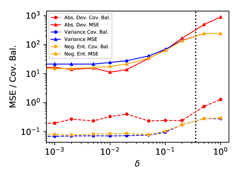
(a) Good overlap

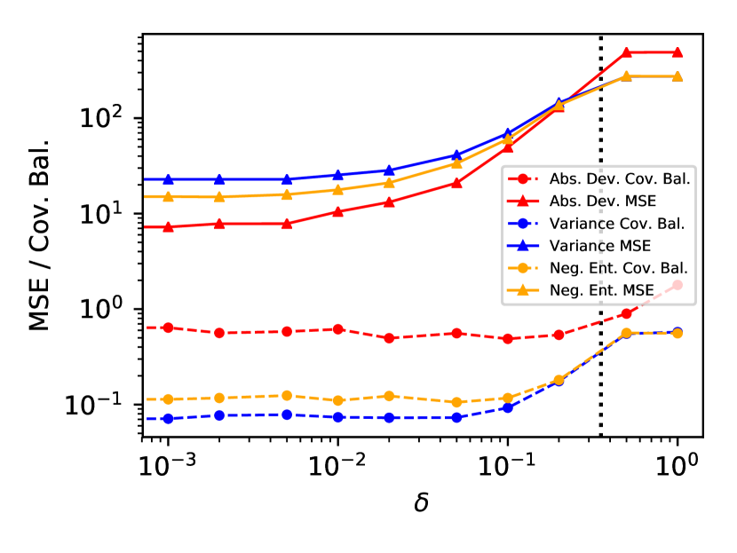
(b) Bad overlap

Figure 2: Bootstrapped covariate balance $C_{S}$ and mean squared error for different values of $\delta$ for the average treatment effect on the treated in the Kang and Shafer study. Using $C_{S}$ to select $\delta$ as in Algorithm 1 coincides with or neighbors the optimal $\delta$ with the smallest error. (The horizontal axis start from $\delta=0$. The vertical dotted line indicates $\delta=K^{-1/2}$, where $K$ is the number of covariates being balanced. We recommend not choosing $\delta$’s bigger than $K^{-1/2}$ because they likely break the assumptions required by the asymptotics. )

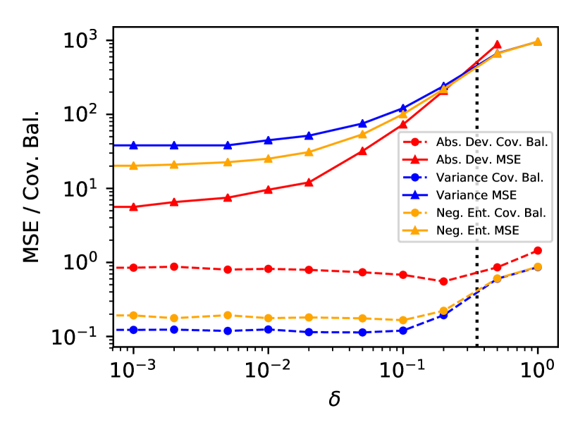
(a) Good overlap

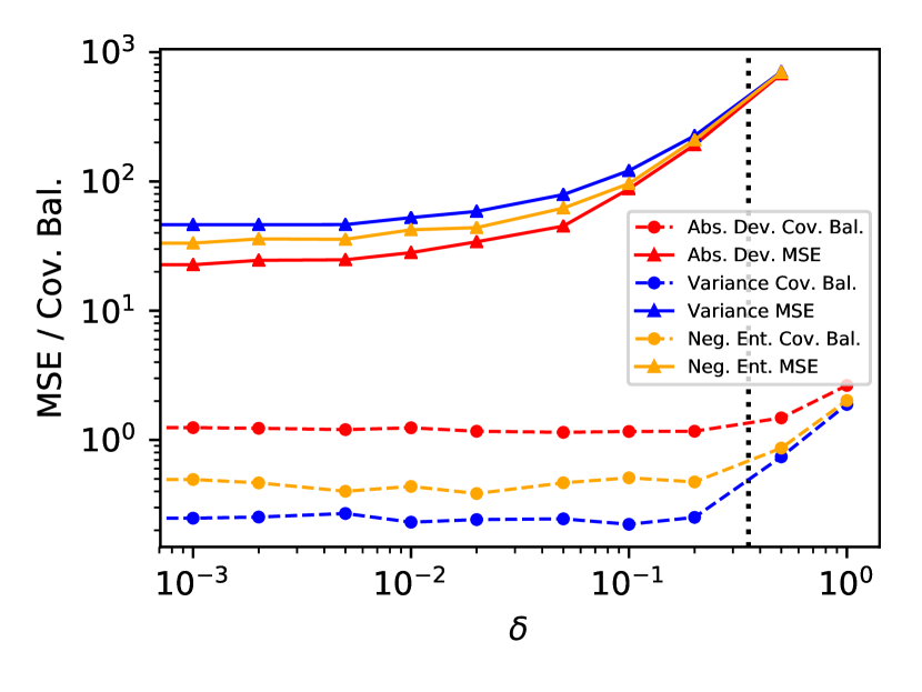
(b) Bad overlap

Figure 3: Bootstrapped covariate balance $C_{S}$ and mean squared error for different values of $\delta$ for the average treatment effect on the treated in the Kang and Shafer study. Using $C_{S}$ to select $\delta$ as in Algorithm 1 coincides with or neighbors the optimal $\delta$ with the smallest error. (The horizontal axis start from $\delta=0$. The vertical dotted line indicates $\delta=K^{-1/2}$, where $K$ is the number of covariates being balanced. We recommend not choosing $\delta$’s bigger than $K^{-1/2}$ because they likely break the assumptions required by the asymptotics. )

D.3 The LaLonde Data Set

We next study the performance of minimal weights in the LaLonde data set (LaLonde, 1986). This data set has two components: an experimental part from a randomized experiment evaluating a large scale job training program (the National Supported Work Demonstration, NSW) on 185 participants; and an observational part, where the experimental control group from the randomized experiment is replaced by a control group of 15992 of nonparticipants drawn from the Current Population Survey (CPS). The experimental part provides a benchmark for the effect of the job training program to be recovered from observational part of the data set. This benchmark is $1794 for the average treatment effect on the treated with a 95% confidence interval of $[551,3038]$.

Table 3 presents the average treatment effect on the treated estimates and their 95% confidence intervals using minimal weights and its exact balancing counterpart. We use $\delta\cdot$sd for different levels of approximate balancing. Minimal weights together with the tuning algorithm produces more efficient mean average treatment effect on the treated estimates while remaining close to the experimental target $1794. The 95% confidence intervals all contain the experimental 95% confidence interval and they become more efficient as $\delta$ increases. When $\delta$ grows to as large as 1 sd, the average treatment effect on the treated estimates starts to shift away from the target. This is intuitive as overly large $\delta$ would imply we are no longer balancing the covariates. In this regard, we conclude minimal weights produce more efficient average treatment effect on the treated estimates while being faithful to the truth (experimental target).

Minimize	Exact	Approx.
Absolute Deviation	712 (2602)	744 (1257)
Variance	1668 (1076)	1387 (886)
Negative Entropy	1706 (958)	1382 (1078)

Table 3: Average treatment effect on the treated estimates in the Lalonde study. (We present the estimates as mean(sd).) Minimal weights produce more efficient estimates while being faithful to the truth.

D.4 The Wong and Chan Simulation

We finally study the minimal weights in the Wong and Chan (2018) simulation. It starts with a ten-dimensional multivariate standard Gaussian random vector $Z=(Z_{1},\ldots,Z_{10})^{\top}$ for each observation. Then it generates ten observed covariates $X=(X_{1},\ldots,X_{10})^{\top},$ where

$$X_{1}=\exp(Z_{1}/2),$$

$$X_{2}=Z_{2}/\{1+\exp(Z_{1})\},$$

$$X_{3}=(Z_{1}Z_{3}/25+0.6)^{3},$$

$$X_{4}=(Z_{2}+Z_{4}+20)^{2},$$

$$X_{j}=Z_{j},j=5,\ldots,10.$$

The propensity score model is

$$\mathrm{pr}(T=1\,|\,Z)=\exp(-Z_{1}-0.1Z_{4})/\{1+\exp(-Z_{1}-0.1Z_{4})\}.$$

The study considers two outcome regression models. Model A is

$$Y=210+(1.5T-0.5)(27.4Z_{1}+13.7Z_{2}+13.7Z_{3}+13.7Z_{4})+\epsilon,$$

and model B is

$$Y=Z_{1}Z_{2}^{3}Z_{3}^{2}Z_{4}+Z_{4}|Z_{1}|^{0.5}+\epsilon,$$

where $\epsilon\sim N(0,1).$

We generate a dataset of size $N=5000$ and study both the average treatment effect and the average treatment effect on the treated estimates. (We take the size of the bootstrap samples as 1/10 of the original sample size. We default to 10 bootstrap samples for covariate balance evaluation. We balance the first and second moments of the covariates.)

Tables 4 presents the root mean squared error of the weighting mean estimates. Approximate balancing with Algorithm 1 outperforms exact balancing in many cases, especially in estimating the average treatment effect. The performance is less stable with the outcome model A, where it could lead to suboptimal performance. When the treatment indicator interacts with potential confounders $Z$’s, classical bootstrap agnostic to the treatment indicator does not serve as a good indicator of downstream estimation performance. Figure 4 shows the mean squared error versus bootstrapped covariate balance plot. The pattern of bootstrapped covariate balance roughly aligns with the mean squared error. This implies that selecting $\delta$ with Algorithm 1 (i.e. selecting according to the bootstrapped covariate balance) could often result in close-to-optimal error, especially in estimating the average treatment effect.

	Outcome model A			Outcome model B
Minimize	Exact	Approx.		Exact	Approx.
Absolute Deviation	0.67	0.66		0.26	0.26
Variance	0.72	0.79		0.26	0.25
Negative Entropy	0.78	0.89		0.25	0.25

(a) Average treatment effect on the treated

	Outcome model A			Outcome model B
Minimize	Exact	Approx.		Exact	Approx.
Absolute Deviation	0.47	0.45		0.23	0.24
Variance	1.35	0.51		0.31	0.21
Negative Entropy	0.44	0.52		0.21	0.21

(b) Average treatment effect

Table 4: Root mean squared error in the Wong-Chan study. Approximate balancing often produce similar-or-better quality estimates than exact balancing.

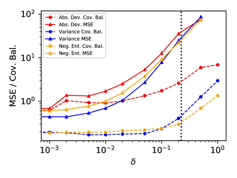
(a) Average treatment effect on the treated

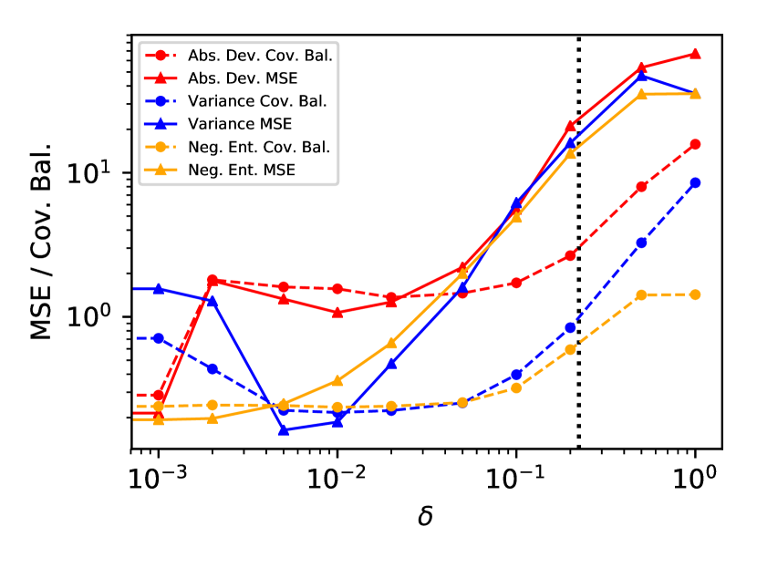
(b) Average treatment effect

Figure 4: Bootstrapped covariate balance $C_{S}$ and mean squared error for different values of $\delta$ for the average treatment effect on the treated in the Wong and Chan study. Using $C_{S}$ to select $\delta$ as in Algorithm 1 coincides with or neighbors the optimal $\delta$ with the smallest error, especially in estimating the average treatment effect. (The horizontal axis start from $\delta=0$. The vertical dotted line indicates $\delta=K^{-1/2}$, where $K$ is the number of covariates being balanced. We recommend not choosing $\delta$’s bigger than $K^{-1/2}$ because they likely break the assumptions required by the asymptotics. )

References

- Abadie and Imbens (2006) Abadie, A. and Imbens, G. W. (2006). Large sample properties of matching estimators for average treatment effects. Econometrica, 74(1):235–267.
- Athey et al. (2018) Athey, S., Imbens, G. W., and Wager, S. (2018). Approximate residual balancing: De-biased inference of average treatment effects in high dimensions. Journal of the Royal Statistical Society: Series B.
- Belloni et al. (2015) Belloni, A., Chernozhukov, V., Chetverikov, D., and Kato, K. (2015). Some new asymptotic theory for least squares series: Pointwise and uniform results. Journal of Econometrics, 186(2):345–366.
- Boyd and Vandenberghe (2004) Boyd, S. and Vandenberghe, L. (2004). Convex Optimization. Cambridge University Press.
- Chan et al. (2016) Chan, K. C. G., Yam, S. C. P., and Zhang, Z. (2016). Globally efficient nonparametric inference of average treatment effects by empirical balancing calibration weighting. Journal of the Royal Statistical Society: Series B, 78(3):673–700.
- Chen (2007) Chen, X. (2007). Large sample sieve estimation of semi-nonparametric models. Handbook of Econometrics, 6:5549–5632.
- Connors et al. (1996) Connors, A. F., Speroff, T., Dawson, N. V., Thomas, C., Harrell, F. E., Wagner, D., Desbiens, N., Goldman, L., Wu, A. W., Califf, R. M., et al. (1996). The effectiveness of right heart catheterization in the initial care of critically ill patients. Journal of the American Medical Association, 276(11):889–897.
- De Boor (1972) De Boor, C. (1972). On calculating with b-splines. Journal of Approximation Theory, 6(1):50–62.
- Deville and Särndal (1992) Deville, J.-C. and Särndal, C.-E. (1992). Calibration estimators in survey sampling. Journal of the American Statistical Association, 87(418):376–382.
- Diamond and Sekhon (2013) Diamond, A. and Sekhon, J. S. (2013). Genetic matching for estimating causal effects: A general multivariate matching method for achieving balance in observational studies. Review of Economics and Statistics, 95(3):932–945.
- Fan et al. (2016) Fan, J., Imai, K., Liu, H., Ning, Y., and Yang, X. (2016). Improving covariate balancing propensity score: A doubly robust and efficient approach.
- Hahn (1998) Hahn, J. (1998). On the role of the propensity score in efficient semiparametric estimation of average treatment effects. Econometrica, pages 315–331.
- Hainmueller (2012) Hainmueller, J. (2012). Entropy balancing for causal effects: a multivariate reweighting method to produce balanced samples in observational studies. Political Analysis, 20(1):25–46.
- Hansen (2004) Hansen, B. B. (2004). Full matching in an observational study of coaching for the SAT. Journal of the American Statistical Association, 99(467):609–618.
- Hellerstein and Imbens (1999) Hellerstein, J. K. and Imbens, G. W. (1999). Imposing moment restrictions from auxiliary data by weighting. Review of Economics and Statistics, 81(1):1–14.
- Hirano et al. (2003) Hirano, K., Imbens, G. W., and Ridder, G. (2003). Efficient estimation of average treatment effects using the estimated propensity score. Econometrica, 71(4):1161–1189.
- Hirshberg and Wager (2018) Hirshberg, D. A. and Wager, S. (2018). Augmented minimax linear estimation. arXiv:1712.00038.
- Horowitz et al. (2004) Horowitz, J. L., Mammen, E., et al. (2004). Nonparametric estimation of an additive model with a link function. Annals of Statistics, 32(6):2412–2443.
- Imai and Ratkovic (2014) Imai, K. and Ratkovic, M. (2014). Covariate balancing propensity score. Journal of the Royal Statistical Society: Series B, 76(1):243–263.
- Kallus (2016) Kallus, N. (2016). Generalized optimal matching methods for causal inference. arXiv:1612.08321.
- Kang and Schafer (2007) Kang, J. D. Y. and Schafer, J. L. (2007). Demystifying double robustness: A comparison of alternative strategies for estimating a population mean from incomplete data (with discussion). Statistical Science, 22(4):523–539.
- Kennedy (2016) Kennedy, E. H. (2016). Semiparametric theory and empirical processes in causal inference. In Statistical Causal Inferences and Their Applications in Public Health Research, pages 141–167. Springer.
- LaLonde (1986) LaLonde, R. J. (1986). Evaluating the econometric evaluations of training programs with experimental data. The American Economic Review, pages 604–620.
- Li et al. (2018) Li, F., Morgan, K. L., and Zaslavsky, A. M. (2018). Balancing covariates via propensity score weighting. Journal of the American Statistical Association, 113(521):390–400.
- Little and Rubin (2014) Little, R. J. and Rubin, D. B. (2014). Statistical analysis with missing data. John Wiley & Sons.
- Newey (1997) Newey, W. K. (1997). Convergence rates and asymptotic normality for series estimators. Journal of Econometrics, 79(1):147–168.
- Robins et al. (2007) Robins, J., Sued, M., Lei-Gomez, Q., and Rotnitzky, A. (2007). Comment: Performance of double-robust estimators when" inverse probability" weights are highly variable. Statistical Science, 22(4):544–559.
- Robins and Gill (1997) Robins, J. M. and Gill, R. D. (1997). Non-response models for the analysis of non-monotone ignorable missing data. Statistics in medicine, 16(1):39–56.
- Robins and Rotnitzky (1995) Robins, J. M. and Rotnitzky, A. (1995). Semiparametric efficiency in multivariate regression models with missing data. Journal of the American Statistical Association, 90(429):122–129.
- Robins et al. (1994) Robins, J. M., Rotnitzky, A., and Zhao, L. P. (1994). Estimation of regression coefficients when some regressors are not always observed. Journal of the American Statistical Association, 89(427):846–866.
- Rosenbaum (1987) Rosenbaum, P. R. (1987). Model-based direct adjustment. Journal of the American Statistical Association, 82(398):387–394.
- Rosenbaum (1989) Rosenbaum, P. R. (1989). Optimal matching for observational studies. Journal of the American Statistical Association, 84:1024–1032.
- Rosenbaum (2010) Rosenbaum, P. R. (2010). Design of Observational Studies. Springer.
- Rosenbaum and Rubin (1983) Rosenbaum, P. R. and Rubin, D. B. (1983). The central role of the propensity score in observational studies for causal effects. Biometrika, 70(1):41–55.
- Rubin (1973) Rubin, D. B. (1973). Matching to remove bias in observational studies. Biometrics, 29:159–183.
- Rubin (2008) Rubin, D. B. (2008). For objective causal inference, design trumps analysis. Annals of Applied Statistics, 2(3):808–840.
- Singh and Tiwari (2006) Singh, B. N. and Tiwari, A. K. (2006). Optimal selection of wavelet basis function applied to ecg signal denoising. Digital signal processing, 16(3):275–287.
- Tropp et al. (2015) Tropp, J. A. et al. (2015). An introduction to matrix concentration inequalities. Foundations and Trends® in Machine Learning, 8(1-2):1–230.
- Tseng and Bertsekas (1987) Tseng, P. and Bertsekas, D. P. (1987). Relaxation methods for problems with strictly convex separable costs and linear constraints. Mathematical Programming, 38(3):303–321.
- Tseng and Bertsekas (1991) Tseng, P. and Bertsekas, D. P. (1991). Relaxation methods for problems with strictly convex costs and linear constraints. Mathematics of Operations Research, 16(3):462–481.
- Van de Geer (2008) Van de Geer, S. A. (2008). High-dimensional generalized linear models and the lasso. Annals of Statistics, pages 614–645.
- Van Der Vaart and Wellner (1996) Van Der Vaart, A. W. and Wellner, J. A. (1996). Weak convergence. In Weak Convergence and Empirical Processes, pages 16–28. Springer.
- Wong and Chan (2018) Wong, R. K. and Chan, K. C. G. (2018). Kernel-based covariate functional balancing for observational studies. Biometrika, 105(1):199–213.
- Yiu and Su (2018) Yiu, S. and Su, L. (2018). Covariate association eliminating weights: a unified weighting framework for causal effect estimation. Biometrika.
- Zhao (2018) Zhao, Q. (2018). Covariate balancing propensity score by tailored loss functions. Annals of Statistics, page in press.
- Zhao and Percival (2017) Zhao, Q. and Percival, D. (2017). Entropy balancing is doubly robust. Journal of Causal Inference, 5(1).
- Zubizarreta (2012) Zubizarreta, J. R. (2012). Using mixed integer programming for matching in an observational study of kidney failure after surgery. Journal of the American Statistical Association, 107(500):1360–1371.
- Zubizarreta (2015) Zubizarreta, J. R. (2015). Stable weights that balance covariates for estimation with incomplete outcome data. Journal of the American Statistical Association, 110(511):910–922.
- Zubizarreta et al. (2011) Zubizarreta, J. R., Reinke, C. E., Kelz, R. R., Silber, J. H., and Rosenbaum, P. R. (2011). Matching for several sparse nominal variables in a case-control study of readmission following surgery. The American Statistician, 65(4):229–238.