Variable selection in model-based clustering and discriminant analysis with a regularization approach

Abstract

Relevant methods of variable selection have been proposed in model-based clustering and classification. These methods are making use of backward or forward procedures to define the roles of the variables. Unfortunately, these stepwise procedures are terribly slow and make these variable selection algorithms inefficient to treat large data sets. In this paper, an alternative regularization approach of variable selection is proposed for model-based clustering and classification. In this approach, the variables are first ranked with a lasso-like procedure in order to avoid painfully slow stepwise algorithms. Thus, the variable selection methodology of Maugis et al (2009b) can be efficiently applied on high-dimensional data sets.

1 Introduction

In data mining and statistical learning, available datasets are larger and larger. As a result, there is more and more interest in variable selection procedures for clustering and classification tasks. After a series of papers on variable selection in model-based clustering (Law et al, 2004; Tadesse et al, 2005; Raftery and Dean, 2006; Maugis et al, 2009a), Maugis et al (2009b) proposed a general model for selecting variables for clustering with Gaussian mixtures. This model, called SRUW, distinguishes between relevant variables $(S)$ and irrelevant variables $(S^{c})$ for clustering. In addition, the irrelevant variables are divided into two categories. A part of the irrelevant variables $(U)$ may be dependent on a subset $R$ of the relevant variables and an other part $(W)$ are independent of other variables. In Maugis et al (2009b), a procedure using embedded stepwise variable selection algorithms is used to identify the SRUW sets. It leads to compare two models at each step in order to determine which variable should be excluded or included in the set $S$, $R$, $U$ or $W$. But these stepwise procedures implemented in SelvarClustIndep , are limited as soon as the number of variables is of the order of a few tens. The SRUW model has been adapted to the Gaussian model-based classification framework in Maugis et al (2011), see also Murphy et al (2010). In this supervised framework, the identification of the sets $S$, $R$, $U$ and $W$ is simpler since the stepwise procedures are not performed inside an EM algorithm but the stepwise algorithms still encounters combinatorial explosion phenomenons.

In parallel Pan and Shen (2007) were inspired by the success of the lasso regression to develop a method of variable selection in model-based clustering using $\ell_{1}$ regularization of the likelihood. This approach was successively extended in Xie et al (2008); Wang and Zhu (2008) and finally Zhou et al (2009) proposed a regularized Gaussian mixture model with unconstrained covariance matrices.

In the present paper, the variables are first ranked using a $\ell_{1}$ penalty placed on the Gaussian mixture component mean vectors and precision matrices. This is made feasible by exploiting the abundant literature on lasso penalization in Gaussian graphical models (see Friedman et al, 2007; Meinshausen and Bühlmann, 2006). Using the resulting ranking of the variables avoids combinatorial problems of the stepwise variable selection algorithms. And, it is hoped that using this lasso-like ranking of the variables instead of stepwise algorithms would not deteriorate the identification of the sets $S$, $R$, $U$ and $W$.

This article is organized as follows. In Section 2, the SRUW model is reviewed in the Gaussian model-based clustering context and its simple extension to the Gaussian model-based classification context is sketched. The variable selection procedure using lasso-like penalization is presented in Section 3 focusing on model-based clustering. Section 4 is devoted to the comparison of the procedures SelvarClustIndep and SelvarMix on several simulated datasets. A short discussion section ends the article.

2 The SRUW model

2.1 Model-based clustering

Let $n$ observations $\mathbf{y}=(\mathbf{y}_{1},\ldots,\mathbf{y}_{n})^{\prime}$ be described by $p$ continuous variables ($\mathbf{y}_{i}\in\mathbb{R}^{p}$). In the model-based clustering framework, the multivariate continuous data $\mathbf{y}$ are assumed to come from several subpopulations (clusters) modeled with a multivariate Gaussian density. The observations are assumed to arise from a finite Gaussian mixture with $K$ components and a mixture form $m$, namely

$$f\big{(}\mathbf{y}_{i}\mid K,m,\alpha\big{)}=\underset{k=1}{\stackrel{{\scriptstyle K}}{{\sum}}}\pi_{k}\phi\big{(}\mathbf{y}_{i}\mid\mu_{k},\Sigma_{k(m)}\big{)},$$

where $\boldsymbol{\pi}=(\pi_{1},\ldots,\pi_{K})$ is the mixing proportion vector ($\pi_{k}\in(0,1)$ for all $k=1,\ldots,K$ and $\sum_{k=1}^{K}\pi_{k}=1$), $\phi\big{(}\cdot\mid\mu_{k},\Sigma_{k}\big{)}$ is the $p$-dimensional Gaussian density function with mean $\mu_{k}$ and covariance matrix $\Sigma_{k}$, and $\alpha=\big{(}\boldsymbol{\pi},\mu_{1},\ldots,\mu_{K},\Sigma_{1},\ldots,\Sigma_{K}\big{)}$ is the parameter vector. Several Gaussian mixture forms $m$ are available, each corresponding to different assumptions on the forms of the covariance matrices, arising from a modified spectral decomposition. These include whether the volume, shape and orientation of each mixture component vary between components or are constant across clusters (Banfield and Raftery, 1993; Celeux and Govaert, 1995).

Typically, the mixture parameters are estimated via maximum likelihood using the EM algorithm (Dempster et al, 1977), and both the number of components $K$ and the mixture form $m$ are chosen using the Bayesian Information Criterion (BIC) (Schwarz, 1978) or other penalized likelihood criteria as the Integrated Completed Likelihood (ICL) criterion (Biernacki et al, 2000) in the clustering context. Among the R packages which implement this methodology, we could mention the mclust (Scrucca et al, 2016) software, and the Rmixmod (Lebret et al, 2015) software.

2.2 Variable selection in model-based clustering

The SRUW model, as described in Maugis et al (2009b), involves three possible roles for the variables: the relevant clustering variables ($S$), the redundant variables ($U$) and the independent variables ($W$). Moreover, the redundant variables $U$ are explained by a subset $R$ of the relevant variables $S$, while the variables $W$ are assumed to be independent of the relevant variables. Thus the data density is assumed to be decomposed into three parts as follows:

$$f(\mathbf{y}_{i}\mid K,m,r,\ell,\mathbf{V},\theta)=$$

$$\underset{k=1}{\stackrel{{\scriptstyle K}}{{\sum}}}\pi_{k}\phi\left(\mathbf{y}_{i}^{S}\mid\mu_{k},\Sigma_{k(m)}\right)\times\phi\left(\mathbf{y}_{i}^{U}\mid a+\mathbf{y}_{i}^{R}b,\Omega_{(r)}\right)\times\phi\left(\mathbf{y}_{i}^{W}\mid\gamma,\tau_{(\ell)}\right)$$

where $\theta=(\alpha,a,b,\Omega,\gamma,\tau)$ is the full parameter vector and $\mathbf{V}=(S,R,U,W)$. The form of the regression covariance matrix $\Omega$ is denoted by $r$; it can be spherical, diagonal or general. The form of the covariance matrix $\tau$ of the independent variables $W$ is denoted by $\ell$ and can be spherical or diagonal.

The SRUW model recasts the variable selection problem for model-based clustering as a model selection problem, where the model collection is indexed by $(K,m,r,\ell,S,R,U,W)$. This model selection problem is solved maximizing the following BIC-type criterion:

$$\mbox{crit}\big{(}K,m,r,\ell,\mathbf{V}\big{)}=$$

$$\mbox{BIC}_{\text{clust}}\left(\mathbf{y}^{S}\mid K,m\right)+\mbox{BIC}_{\text{reg}}\left(\mathbf{y}^{U}\mid r,\mathbf{y}^{R}\right)+\mbox{BIC}_{\text{indep}}\left(\mathbf{y}^{W}\mid\ell\right),$$ (1)

where $\mbox{BIC}_{\text{clust}}$ represents the BIC criterion of the Gaussian mixture model with the variables $S$, $\mbox{BIC}_{\text{reg}}$ represents the BIC criterion of the regression model of the variables $U$ on the variables $R$ and $\mbox{BIC}_{\text{indep}}$ represents the BIC criterion of the Gaussian model with the variables $W$.

Since the SRUW model collection is large, two embedded backward or forward stepwise algorithms for variable selection, one for the clustering and one for the linear regression, are considered to solve this model selection problem. A backward algorithm allows one to start with all variables in order to take variable dependencies into account. A forward procedure, starting with an empty clustering variable set or a small variable subset, could be preferred for numerical reasons when the number of variables is large. The method is implemented in the SelvarClustIndep software and a simplified version is implemented in the clustvarsel R package. But in a high-dimensional setting, even the variable selection method with the two forward stepwise algorithms becomes painfully slow and alternative methods are desirable.

2.3 Variable selection in Classification

In the supervised classification framework, the labels of the training dataset are known and the variable selection problem is analogous but simpler than in the clustering framework. The training data set is

$$(\mathbf{y},\mathbf{z})=\{(\mathbf{y}_{1},z_{1}),\ldots,(\mathbf{y}_{n},z_{n});\ \mathbf{y}_{i}\in\mathbb{R}^{p},z_{i}\in\{1,\ldots,K\}\},$$

where $\mathbf{y}_{i}$ is the $p$-dimensional i.i.d predictors and $z_{i}$ are the corresponding class labels. The number of classes $K$ is known. The subset $S$ is now the discriminant variable subset. Under a model $(m,r,\ell,\mathbf{V})$ with $\mathbf{V}=(S,R,U,W)$, the distribution of the training sample is modeled by

$$\left\{\begin{array}[]{r c l}f(\mathbf{y}_{i}|z_{i}=k,m,r,\ell,\mathbf{V})&=&\phi(\mathbf{y}_{i}^{S}|\mu_{k},\Sigma_{k(m)})\,\phi(\mathbf{y}_{i}^{U}|a+\mathbf{y}^{R}\beta,\Omega_{(r)})\,\phi(\mathbf{y}_{i}^{W}|\gamma,\tau_{(\ell)})\\ \\ (\mathds{1}_{z_{i}=1},\ldots,\mathds{1}_{z_{i}=K})&\sim&\mbox{Multinomial}(1;\pi_{1},\ldots,\pi_{K})\end{array}.\right.$$

According to the assumed form of the covariance matrices involving their eigenvalue decomposition, a collection of more or less parsimonious mixture forms $(m)$ is available as in the clustering context.

Considering the same model SRUW, the variable selection problem is solved by using the following model selection criterion

$$\mbox{crit}(m,r,\ell,\mathbf{V})=\mbox{BIC}_{\text{clas}}(\mathbf{y}^{S},\mathbf{z}|m)+\mbox{BIC}_{\text{reg}}(\mathbf{y}^{U}|r,\mathbf{y}^{R})+\mbox{BIC}_{\text{indep}}(\mathbf{y}^{W}|\ell),$$

where $\mbox{BIC}_{\text{clas}}$ denotes the BIC criterion for the Gaussian classification on the discriminant variable subset $S$. Maximizing this criterion is an easier task in this supervised context since there is no need to use the EM algorithm to derive the parameter estimates of the Gaussian classification model contrary to the model-based clustering situation. See Maugis et al (2011) for details. But, the variable selection procedure with two embedded stepwise procedures remain expensive and alternative procedures are desirable.

3 Variable selection through regularization

In order to avoid the highly CPU-time consuming of stepwise algorithms, we propose an alternative variable selection procedure in two steps: First, the variables are ranked through a lasso-like procedure, and second, the variable roles are determined using criterion (1) on these ranked variables. The procedure is detailed in the clustering framework, the simplifications for classification are presented in Section 3.3. This variable selection procedure is implemented in the R package SelvarMix.

3.1 Variable ranking by regularization

In the first step, the variables are ranked through the lasso-like procedure of Zhou et al (2009). For any $K\in\mathbb{N}^{\star}$, the criterion to be maximized is

$$\sum_{i=1}^{n}\ln\Big{[}\sum_{k=1}^{K}\pi_{k}\phi\big{(}\bar{\mathbf{y}}_{i}\mid\mu_{k},\Sigma_{k}\big{)}\Big{]}-\lambda\sum^{K}_{k=1}\left\|\mu_{k}\right\|_{1}-\rho\sum_{k=1}^{K}\left\|\Sigma_{k}^{-1}\right\|_{1},$$ (2)

where

$$\left\|\mu_{k}\right\|_{1}=\underset{j=1}{\stackrel{{\scriptstyle p}}{{\sum}}}\big{|}\mu_{kj}\big{|},\left\|\Sigma_{k}^{-1}\right\|_{1}=\underset{j^{\prime}\neq j}{\sum_{j^{\prime}=1}^{p}\sum_{j=1}^{p}}\left|(\Sigma_{k}^{-1})_{jj^{\prime}}\right|,$$

$\bar{\mathbf{y}}_{i}=(y_{ij}-\bar{\mathbf{y}}_{j})_{1\leq j\leq p}$ with $\bar{\mathbf{y}}_{j}=\frac{1}{n}\sum_{i=1}^{n}y_{ij}$ and where $\lambda$ and $\rho$ are two non negative regularization parameters defined on two grids of values $\mathcal{G}_{\lambda}$ and $\mathcal{G}_{\rho}$ respectively. The estimated mixture parameters for fixed tuning parameters $\lambda$ and $\rho$,

$$\widehat{\alpha}(\lambda,\rho)=\big{(}\widehat{\boldsymbol{\pi}}(\lambda,\rho),\widehat{\mu}_{1}(\lambda,\rho),\ldots,\widehat{\mu}_{K}(\lambda,\rho),\widehat{\Sigma}_{1}(\lambda,\rho),\ldots,\widehat{\Sigma}_{K}(\lambda,\rho)\big{)}$$

are computed with the EM algorithm of Zhou et al (2009). In particular, the glasso algorithm (Friedman et al, 2007) using a coordinate descent procedure for the lasso is used to estimate the sparse precision matrices $\Sigma_{k}^{-1},k=1,\ldots,K$. This procedure is reminded in Appendix A.1.

It is worth noting that this lasso-like criterion does not take into account the typology of the variables induced by the SRUW model. Strictly speaking, it only distinguishes two possible roles for the variables: a variable is declared related or independent of the clustering. A variable is declared independent for the clustering if for all $j=1,\ldots,p$, and $k=1,\ldots,K$, $\widehat{\mu}_{k}(\lambda,\rho)=0$. The variance matrices are not considered in this definition. Actually, their role is secondary in clustering and taking them into account would imply serious numerical difficulties.

Varying the regularization parameters $(\lambda,\rho)$ in $\mathcal{G}_{\lambda}\times\mathcal{G}_{\rho}$, a ”clustering” score is defined for each variable $j\in\{1,\ldots,p\}$ and for fixed $K$ by

$$\mathcal{O}_{K}(j)=\sum_{(\lambda,\rho)\in\mathcal{G}_{\lambda}\times\mathcal{G}_{\rho}}{\mathcal{B}}_{(K,\rho,\lambda)}(j)$$

where

$${\mathcal{B}}_{(K,\rho,\lambda)}(j)=\begin{cases}0&\mbox{if }\widehat{\mu}_{1j}(\lambda,\rho)=\ldots=\widehat{\mu}_{Kj}(\lambda,\rho)=0\\ 1&\mbox{else}.\end{cases}$$

The larger $\mathcal{O}_{K}(j)$ is the more related to the clustering the variable $j$ is expected to be. The variables are thus ranked by their decreasing values on $\mathcal{O}_{K}(j)$. This variable ranking is denoted $\mathcal{I}_{K}=(j_{1},\ldots,j_{p})$ with $\mathcal{O}_{K}(j_{1})>\mathcal{O}_{K}(j_{2})>\ldots>\mathcal{O}_{K}(j_{p})$.

3.2 Determination of the variable roles

The relevant clustering variable set $S_{(K,m)}$ is determined first. The variable set is scanned according to the $\mathcal{I}_{K}$ order. One variable is added to $S_{(K,m)}$ if

$$\mbox{BIC}_{\text{diff}}(j_{v}) = \mbox{BIC}_{\text{clust}}\Big{(}\mathbf{y}^{S_{(K,m)}},\mathbf{y}^{j_{v}}\mid K,m\Big{)}$$ (3)

$$-\mbox{BIC}_{\text{clust}}\Big{(}\mathbf{y}^{S_{(K,m)}}\mid K,m\Big{)}-\mbox{BIC}_{\text{reg}}\Big{(}\mathbf{y}^{j_{v}}\mid\mathbf{y}^{R[j_{v}]}\Big{)}$$

is positive, $R[j_{v}]$ being the variables of $S_{(K,m)}$ required to linearly explain $\mathbf{y}^{j_{v}}$. This subset $R[j_{v}]$ is determined with standard backward stepwise algorithm for variable selection in linear regression. The scanning of $\mathcal{I}_{K}$ is stopped as soon as $c$ successive variables have a non positive $\mbox{BIC}_{\text{diff}}$ value, $c$ being a fixed positive integer. Once the relevant variable set $S_{(K,m)}$ is determined, the independent variable set $W$ is determined as follows. Scanning the variable set according to the reverse order of $I_{K}$, a variable $j_{v}$ is added to $W_{(K,m)}$ if the subset $R[j_{v}]$ of $S_{(K,m)}$ (derived from the backward stepwise algorithm) is empty. The algorithm stops as soon as $c$ successive variables are not declared independent. The redundant variables are thus declared to be $U_{(K,m)}=\{1,\ldots,p\}\setminus\{S_{(K,m)}\cup W_{(K,m)}\}$ and the subset $R_{(K,m,r)}$ of $S_{(K,m)}$ required to linearly explain $\mathbf{y}^{U_{(K,m)}}$ is derived from the backward stepwise algorithm, for each covariance shape $r$. The ideal position of the variable sets $S$, $U$ and $W$ in the variable ranking is schematised in Figure 1. Finally, the model $(\hat{K},\hat{m},\hat{r},\hat{\ell})$ maximizing the criterion $\mbox{crit}\big{(}K,m,r,\ell,\mathbf{V}_{(K,m,r)}\big{)}$ defined in Equation (1) with $\mathbf{V}_{(K,m,r)}=(S_{(K,m)},R_{(K,m,r)},U_{(K,m)},W_{(K,m)})$ is selected.

Figure 1: The ideal position of the sets $S$, $U$ and $W$ in the ranking of the variables

Some comments are in order:

• It is possible to use a lasso procedure instead of the stepwise variable selection algorithm in the linear regression step. However, this replacement is not expected to be highly beneficial since stepwise variable selection in linear regression are not too much expensive and, moreover, the number of variables in the set $S$ is not expected to be high.

• There is no guarantee that the variable order designed in 3.1 would be in accordance with the ideal ranking of the variables displayed in Figure 1. In particular when the variables are highly correlated, lasso-like procedures could be expected to produce confusion between the sets $S$ and $U$. This is the reason why we wait $c\ (>1)$ few steps before deciding the variable roles: we give a chance to the procedure to catch more variables in $S$ and in $W$.

3.3 Variable selection through regularization for classification

In the classification context, $K$ is fixed and the regularization criterion to be maximized is

$$\sum_{i=1}^{n}\sum_{k=1}^{K}\mathds{1}_{\{z_{i}=k\}}\ln\Big{[}\pi_{k}\phi\big{(}\bar{\mathbf{y}}_{i}\mid\mu_{k},\Sigma_{k}\big{)}\Big{]}-\lambda\sum^{K}_{k=1}\left\|\mu_{k}\right\|_{1}-\rho\sum_{k=1}^{K}\left\|\Sigma_{k}^{-1}\right\|_{1},$$ (4)

with the same notation as in Section 3.1. Assuming that the training data set has been obtained according to the mixture sampling scheme, the proportions $\pi_{1},\ldots,\pi_{K}$ are estimated by

$$\widehat{\pi}_{k}=\frac{1}{n}\sum_{i=1}^{n}\mathds{1}_{\{z_{i}=k\}},\ k=1,\ldots,K.$$

The maximization of criterion (4) is done according to the procedure described in Appendix A.2. The only difference with the clustering context is that the labels $z_{i}$ are known and no EM algorithm is required. Thus, a ranking $\mathcal{I}_{K}$ of the variables is get and the procedure described in Section 3.2 for model-based clustering is adapted straightforwardly to the supervised classification context, where (3) is replaced by

$$\mbox{BIC}_{\text{diff}}(j_{v})=$$

$$\mbox{BIC}_{\text{clas}}\left(\mathbf{y}^{S_{(m)}},\mathbf{y}^{j_{v}},\mathbf{z}\mid m\right)-\mbox{BIC}_{\text{clas}}\left(\mathbf{y}^{S_{(m)}},\mathbf{z}\mid m\right)-\mbox{BIC}_{\text{reg}}\left(\mathbf{y}^{j_{v}}\mid\mathbf{y}^{R[j_{v}]}\right).$$

4 Numerical experiments

This section is devoted to comparing our procedure implemented in the R package SelvarMix with the forward/backward stepwise procedures of Maugis et al (2009b, 2011) in both model-based clustering and classification settings.

4.1 Model-based clustering

4.1.1 Comparison on simuated data

We consider one of the seven simulated data sets studied in Maugis et al (2009b, Section 6.1). The data consist of $n=2000$ observations on $p=14$ variables. On the first two variables ($S=\{1,2\}$), data are distributed from an equiprobable mixture of four Gaussian distributions $\mathcal{N}(\mu_{k},I_{2})$ with $\mu_{1}=(0,0),\mu_{2}=(4,0),\mu_{3}=(0,2)$ and $\mu_{4}=(4,2)$. On the nine redundant variables ($U=\{3,\ldots,11\}$), data are simulated as follows: for $i=1,\ldots,n$,

$$\mathbf{y}_{i}^{\{3-11\}}=(0,0,0.4,0.8,\ldots,2)+\mathbf{y}_{i}^{\{1,2\}}b+\varepsilon_{i}$$

where the regression coefficients are

$$b=\big{(}(0.5,1)^{\prime},(2,0)^{\prime},(0,3)^{\prime},(-1,2)^{\prime},(2,-4)^{\prime},(0.5,0)^{\prime},(4,0.5)^{\prime},(3,0)^{\prime},(2,1)^{\prime}\big{)}$$

and $\varepsilon_{i}$ are i.i.i $\mathcal{N}(0_{9},\Omega)$. The regression covariance matrix $\Omega$ is block diagonal

$$\Omega=\text{diag}\big{(}I_{3},0.5I_{2},\Omega_{1},\Omega_{2}\big{)}$$

with $\Omega_{1}=\text{Rot}\big{(}\frac{\pi}{3}\big{)}^{\prime}\text{diag}(1,3)\text{Rot}\big{(}\frac{\pi}{3}\big{)}$ and $\Omega_{2}=\text{Rot}\big{(}\frac{\pi}{6}\big{)}^{\prime}\text{diag}(2,6)\text{Rot}\big{(}\frac{\pi}{6}\big{)}$, where $\text{Rot}(\theta)$ is a plane rotation matrix with angle $\theta$. The last three independent variables are standard Gaussian random variables $\mathbf{y}_{i}^{\{12-14\}}\sim\mathcal{N}\left(0_{3},I_{3}\right)$.

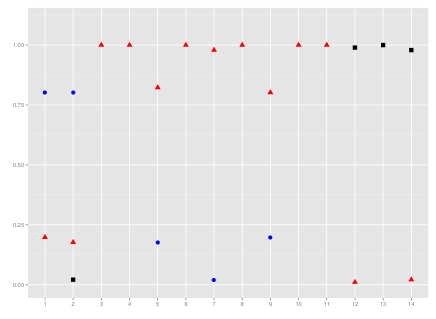
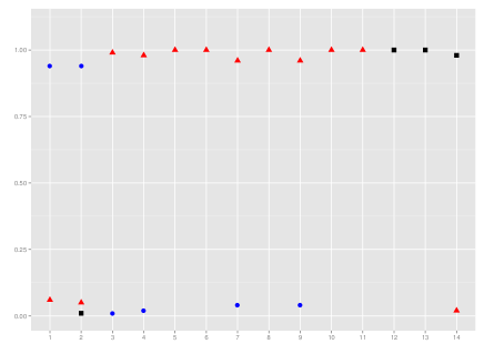
In the first scenario, the function SelvarClustLasso of SelvarMix and the forward Maugis et al (2009b)’s procedure (SelvarClustIndep) are compared on $100$ replications of the simulated dataset with $K=4$ and spherical mixture components. We compare the CPU times of both procedures. The calculations are carried out on an 80 Intel Xeon 2.4 GHz processors machine and the variable ranking procedure (see Section 3.2) of SelvarMix is parallelized. In comparaison to SelvarMix, the combinatorial nature of SelvarClustIndep makes it difficult to be parallelized. As a result, a significant improvement of the runtime with SelvarMix is obtained: SelvarMix takes $47.0(\pm 3.2)$ seconds CPU time whereas SelvarClustIndep needs $450.64(\pm 104.0)$. Figure 2 displays the distribution of the variable roles with SelvarClustIndep in left and SelvarMix in right. Globally, the true variable roles are well recovered. Surprisingly SelvarMix detects the relevant variables better than SelvarClustIndep which sometimes selects variables $5$ and $9$ instead of the first two variables.

Figure 2: Proportion of times each variable was declared relevant (square), redundant (triangle) or independent (circle) by SelvarClustIndep (top) and SelvarMix (bottom) in the first scenario. Zero values are not shown.

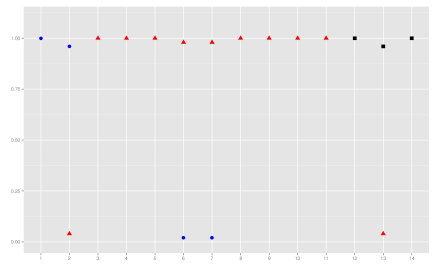
In the second scenario, the 50 previous simulated datasets are considered but now the number of clusters $K$ varies between 2 to 6 and the 28 Gaussian mixture forms $m$ are considered. The true cluster number is always correctly selected by both procedures. The variable selection is similar with both procedures (see Figure 3): the true variable partition is selected 46 (resp. 48) times by SelvarClustIndep (resp. SelvarMix). The clustering performance is preserved with SelvarMix since the average of adjusted rand index (ARI) is $0.6(\pm 0.017)$ with SelvarMix and $0.6(\pm 0.015)$ with SelvarClustIndep.

Figure 3: Proportion of times each variable was declared relevant (square), redundant (triangle) or independent (circle) by SelvarClustIndep (top) and SelvarMix (bottom) in the second scenario. Zero values are not shown.

We also applied the Zhou et al (2009)’s lasso-like procedure on the $50$ simulated datasets. As previously, the number of clusters varies from $2$ to $6$. The penalization parameters, including the means $\widehat{\mu}_{1},\ldots,\widehat{\mu}_{K}$, are estimated according to the penalized likelihood criterion (2) whereas the number of clusters $K$ is selected using the BIC criterion. One variable $j$ is declared relevant if there is at least one cluster $k$ where $|\widehat{\mu}_{kj}|>10^{-1}$. For all $50$ simulated datasets, the Zhou et al (2009)’s procedure fails to select the true number of clusters ($K=4$) and the true set of relevant variables ($S=\{1,2\}$). It always selects $K=6$, both relevant and redundant variables are declared relevant and the ARI is lower ($0.45(\pm 0.025)$).

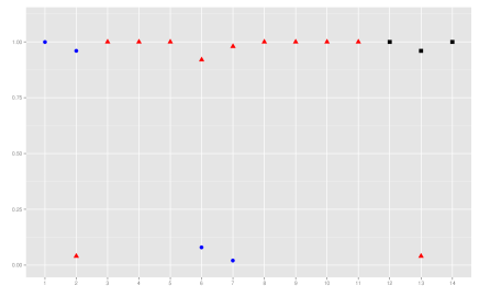
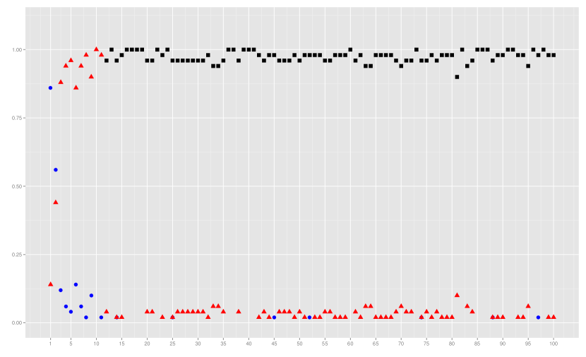
In the third scenario, we consider $50$ datasets consisting of $n=400$ observations described by $100$ variables. On the first eleven variables, data are distributed as previously. Next, 89 standard Gaussian variables are appended. As previously, the number of clusters varies from $2$ to $6$ and the $28$ Gaussian mixtures forms $m$ are considered. The selection of the number of clusters is less efficient: the true cluster number $K=4$ is selected $23$ times, the model with $K=3$ is selected $10$ times whereas the models with $K=2,5$ and $6$ are respectively selected $6,7$ and $4$ times. Compared to the previous scenario in low dimension ($p=14$), the variable selection using SelvarMix is slightly deteriorated (see Figure 4). The true relevant variable set $S=\{1,2\}$ is selected $23$ times. Sometimes, SelvarMix declares one of the redundant variables as relevant. One of the independent variables is declared as relevant seven times. Moreover, the clustering performance is slightly deteriorated: the ARI is $0.49(\pm 0.1)$.

Figure 4: Proportion of times each variable was declared discriminant (square), redundant (triangle) or independent (circle) by SelvarMix in the clustering setting, for the datasets with $p=100$ variables. Zero values are not shown.

4.1.2 Comparison on real datasets

In this section, we compare our proposal with the forward/backward stepwise procedure of Maugis et al (2009b, 2011) on the moderate high-dimensional data sets waveform and transcriptome summarized in Table 1. Results and CPU times are shown in Table 2.

data	$n$	$d$	covariance model	number of components	reference
waveform	$5000$	$41$	20 models	from $3$ to $6$	Maugis et al (2009b)
transcriptome	$4616$	$33$	2 models	from $10$ to $30$	Gagnot et al (2008)

Table 1: Characteristics, references and experiment conditions for both data sets.

data set	Software	BIC	$\widehat{K}$	$\widehat{m}$	$\text{Card}(S)$	$\text{Card}(R)$	$\text{Card}(U)$	$\text{Card}(W)$	time
waveform	SelvarClustIndep	$-591542$	$6$	pkLC	$16$	$8$	$3$	$21$	$>$ 24hrs
	SelvarMix	$-602965$	$6$	pLkC	$15$	$11$	$8$	$18$	$1.29$ mns
transcriptome	SelvarClustIndep	$-694455$	$24$	pkLkC	$30$	$16$	$3$	$0$	$>$ 24 hrs
	SelvarMix	$-695534$	$27$	pkLkC	$29$	$15$	$4$	$0$	1.49 hrs

Table 2: Results and cpu-time for both methods on both data sets.

Table 2 shows that for the transcriptome data set the selected partitions have not the same number of clusters. However, their ARI ($0.60$) is high for a such large number of clusters. Moreover the sets $S,R$ and $U$ are almost identical. Since the CPU time of SelvarMix is dramatically smaller than SelvarClustIndep, this procedure can be preferred.

	SelvarClustIndep
SelvarMix	606	0	0	0	0	1
	0	986	55	0	0	24
	1	0	576	1	0	0
	22	0	19	956	0	0
	61	0	0	0	1063	36
	1	0	1	0	0	591

Table 3: Contingency table of SelvarClustIndep partition vs. SelvarMix partition on the waveform data set. As shown by the table, both partitions are quite similar. The ARI is $0.90$.

4.2 Supervised classification

We consider the same simulated example of Maugis et al (2011). The samples are described by $p=16$ variables. The prior probabilities of the four classes are $\boldsymbol{\pi}=(0.15,0.3,0.2,0.35)$. On the three discriminant variables, data are distributed from

$$\mathbf{y}_{i}^{\{1-3\}}\mid z_{i}=k\sim\mathcal{N}\left(\mu_{k},\Sigma_{k}\right)$$

with means vectors $\mu_{1}=(1.5,-1.5,1.5)$, $\mu_{2}=(-1.5,1.5,1.5)$, $\mu_{3}=(1.5,-1.5,-1.5)$ and $\mu_{4}=(-1.5,1.5,-1.5)$. The covariance matrices are $\Sigma_{k}=\left(\rho_{k}^{|i-j|}\right)$ with $\rho_{1}=0.85,\rho_{2}=0.1,\rho_{3}=0.65$ and $\rho_{4}=0.5$. There are four redundant variables simulated from $\mathbf{y}_{i}^{\{4-7\}}\sim\mathcal{N}\left(\mathbf{y}_{i}^{\{1,3\}}\beta,I_{4}\right).$ with

$$\beta=\left(\begin{array}[]{cccc}1&0&-1&2\\ 0&-2&2&1\end{array}\right).$$

Nine independent variables are appended, sampled from $\mathbf{y}^{\{8-16\}}_{i}\sim\mathcal{N}(\gamma,\tau)$ with

$$\gamma=(-2,-1.5,-1,-0.5,0,0.5,1,1.5,2)$$

and the diagonal matrix

$$\tau=\text{diag}(0.5,0.75,1,1.25,1.5,1.25,1,0.75,0.5).$$

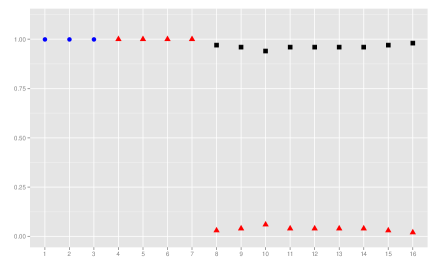
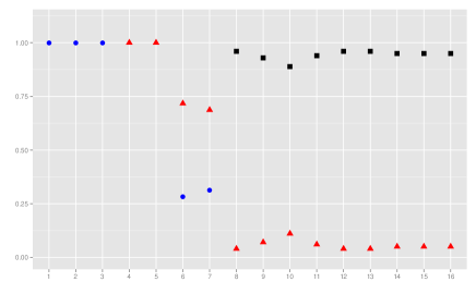
First, $100$ simulation replications are considered where the training sample is composed of $n=500$ observations and the same test sample with $50\,000$ points is used. The fourteen forms $m$ are considered. The two procedures SelvarMix and the version of SelvarClustIndep devoted to the variable selection in supervised classification (which is again called SelvarClustIndep in the sequel) are compared. Figure 5 shows the variable selection obtained with the procedure of Maugis et al (2011) on the left and the SelvarLearnLasso function of SelvarMix on the right. SelvarMix sometimes declares Variables 6 and 7 as relevant with the first three relevant variables and has some tendency to declare redundant some independent variables, more often than SelvarClustIndep. For the prediction, both procedures have a similar behaviour: the misclassification error rate is $4.5\%(\pm 0.19)$ for SelvarMix and $4.18\%(\pm 0.06)$ for SelvarClustIndep.

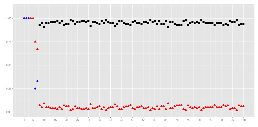
Second, we consider $100$ training samples composed of $n=500$ observations described by $p=100$ variables, $84$ standard Gaussian variables are appended to the previous training samples. The test sample is similarly modified. As expected, SelvarMix allows us to quickly study such data sets where the number of variables is large. The level of prediction is preserved since the misclassification error rate is $4.34\%(\pm 0.18)$ and the variable selection remains similar as shown in Figure 6.

Figure 5: Proportion of times each variable was declared discriminant (square), redundant (triangle) or independent (circle) by SelvarClustIndep (top) and SelvarMix (bottom) in the classification setting, for the data sets with $p=16$ variables. Zero values are not shown.

Figure 6: Proportion of times each variable was declared discriminant (square), redundant (triangle) or independent (circle) by SelvarMix in the classification setting, for the data sets with $p=100$ variables. Zero values are not shown.

5 Discussion

The model SRUW is a powerful model to define the roles of variables in the Gaussian model-based clustering and classification contexts. However the diffusion of this model is slowed down by the stepwise selection algorithms used in its previous implementations. Despite they are sub-optimal these algorithms are highly CPU time demanding.

The regularization approach we propose allows us to avoid these stepwise procedures by designing an irreversible order on which the variables in $S$, $U$ and $W$ are chosen. The numerical experiments performed with the resulting R package SelvarMix show quite encouraging performances. SelvarMix is highly faster than SelvarClustIndep while providing analogous (and sometimes better) performances than the reference SelvarClustIndep program.

In practice the influence of the number $c$ for which the regularization algorithm provides the same role for $c$ successive variables could be regarded as an important tuning parameter. In our numerical experiments, this parameter appears to be not too much sensitive and a default value $c=3$ seems reasonable. However the influence of $c$ needs to be further investigated in order to propose heuristic rules to choose it as a simple function of the total number of variables in a proper way to get stable selections.

Appendix A Procedures to maximize penalized empirical contrasts

A.1 The model-based clustering case

The EM algorithm for maximizing Criterion (2) is as follows (Zhou et al, 2009). The penalized complete loglikelihood of the centered data set $\bar{\mathbf{y}}=\big{(}\bar{\mathbf{y}}_{1},\ldots,\bar{\mathbf{y}}_{n}\big{)}^{\prime}$ is given by

$$L_{\text{c},(\lambda,\rho)}(\bar{\mathbf{y}},\mathbf{z},\alpha)=\sum_{i=1}^{n}\sum_{k=1}^{K}z_{ik}\big{[}\ln(\pi_{k})+\ln\phi(\bar{\mathbf{y}}_{i}\mid\mu_{k},\Sigma_{k})\big{]}-\lambda\sum^{K}_{k=1}\left\|\mu_{k}\right\|_{1}-\rho\sum_{k=1}^{K}\left\|\Theta_{k}\right\|_{1}$$ (5)

where $\Theta_{k}=\Sigma_{k}^{-1}$ denotes the precision matrix of the $k$-th mixture component. The EM algorithm of Zhou et al (2009) maximizes at each iteration the conditional expectation of (5) given $\bar{\mathbf{y}}$ and a current parameter vector $\alpha^{(s)}$: $\mathbb{E}\Big{[}L_{\text{c},(\lambda,\rho)}\big{(}\bar{\mathbf{y}},\mathbf{z},\alpha\big{)}\mid\bar{\mathbf{y}},\alpha^{(s)}\Big{]}.$ The following two steps are repeated from an initial $\alpha^{(0)}$ until convergence. At the $s$-th iteration of the EM algorithm:

• E-step: The conditional probabilities $t^{(s)}_{ik}$ that the $i$-th observation belongs to the $k$-th cluster are computed for $i=1,\ldots,n$ and $k=1,\ldots,K$,

  $$t^{(s)}_{ik}=\mathbb{P}\big{(}z_{ik}=1\mid\bar{\mathbf{y}},\alpha^{(s)}\big{)}=\frac{\pi_{k}^{(s)}\phi\Big{(}\bar{\mathbf{y}}_{i}\mid\mu^{(s)}_{k},\Sigma^{(s)}_{k}\Big{)}}{\sum_{k^{\prime}=1}^{K}\pi_{k^{\prime}}^{(s)}\phi\Big{(}\bar{\mathbf{y}}_{i}\mid\mu^{(s)}_{k^{\prime}},\Sigma^{(s)}_{k^{\prime}}\Big{)}}.$$

• M-step : This step consists of maximizing the expected completed loglikelihood derived from the E-step. It leads to the following mixture parameter updates:

  • The updated proportions are $\pi^{(s+1)}_{k}=\frac{1}{n}\sum_{i=1}^{n}t^{(s)}_{ik}$ for $k=1,\ldots,K$.

  • Compute the updated means $\mu^{(s+1)}_{1},\ldots,\mu^{(s+1)}_{K}$ using the formulas $(14)$ et $(15)$ of Zhou et al (2009): the $j$-th coordinate of $\mu^{(s+1)}_{k}$ is the solution of the following equations

    $$\text{if}\quad\left|\sum_{i=1}^{n}t^{(s)}_{ik}\left[\underset{v\neq j}{\sum_{v=1}^{p}}\left(\bar{\mathbf{y}}_{ij}-\mu^{(s)}_{kv}\right)\Theta^{(s)}_{k,vj}+\bar{\mathbf{y}}_{ij}\Theta^{(s)}_{k,jj}\right]\right|\leq\lambda\quad\text{then}\quad\mu^{(s+1)}_{kj}=0,$$

    otherwise

    $$\left[\sum_{i=1}^{n}t^{(s)}_{ik}\right]\mu^{(s+1)}_{kj}\Theta^{(s)}_{k,jj}+\ \lambda\ \text{sign}\left(\mu^{(s+1)}_{kj}\right) =\sum_{i=1}^{n}t_{ik}^{(s)}\sum_{v=1}^{p}\bar{y}_{iv}\Theta^{(s)}_{k,vj}$$

    $$-\left[\sum_{i=1}^{n}t^{(s)}_{ik}\right]\left[\left(\sum_{v=1}^{p}\mu^{(s)}_{kv}\Theta^{(s)}_{k,vj}\right)-\mu^{(s)}_{kj}\Theta^{(s)}_{k,jj}\right].$$

  • For all $k=1,\ldots,K$, the covariance matrix $\Sigma_{k}^{(s+1)}$ is obtained via the precision matrix $\Theta_{k}^{(s+1)}$. The glasso algorithm (available in the R package glasso of Friedman et al, 2011) is used to solve the following minimization problem on the set of symmetric positive definite matrices (denoted $\Theta\succ 0$):

    $$\underset{\Theta\succ 0}{\mathop{\mathrm{arg\,min}}}\left\{-\ln\text{det}\left(\Theta\right)+\text{trace}\left(S_{k}^{(s+1)}\Theta\right)+\rho_{k}^{(s+1)}\|\Theta\|_{1}\right\},$$

    where $\rho_{k}^{(s+1)}=2\rho\left(\sum_{i=1}^{n}t^{(s)}_{ik}\right)^{-1}$ and

    $$S^{(s+1)}_{k}=\frac{\sum_{i=1}^{n}t^{(s)}_{ik}(\bar{\mathbf{y}}_{i}-\mu^{(s+1)}_{k})(\bar{\mathbf{y}}_{i}-\mu^{(s+1)}_{k})^{\top}}{\sum_{i=1}^{n}t^{(s)}_{ik}}.$$

A.2 The classification case

The maximization of the regularized criterion (4) at $\mu_{1},\ldots,\mu_{K}$ and $\Theta_{1},\ldots,\Theta_{K}$ is achieved using an algorithm similar to the one presented in Section A.1 when the labels $z_{i}$ are known.

The $j$-th coordinate of the mean vector $\mu_{k}$ is the solution of the following equations

$$\text{if}\quad\left|\sum_{i=1}^{n}\mathds{1}_{\{z_{i}=k\}}\left[\underset{v\neq j}{\sum_{v=1}^{p}}\left(\bar{\mathbf{y}}_{ij}-\mu_{kv}\right)\Theta_{k,vj}+\bar{\mathbf{y}}_{ij}\Theta_{k,jj}\right]\right|\leq\lambda\quad\text{then}\quad\mu_{kj}=0,$$

otherwise

$$\left[\sum_{i=1}^{n}\mathds{1}_{\{z_{i}=k\}}\right]\mu_{kj}\Theta_{k,jj}+\lambda\ \text{sign}\left(\mu_{kj}\right) =\sum_{i=1}^{n}\mathds{1}_{\{z_{i}=k\}}\sum_{v=1}^{p}\bar{y}_{iv}\Theta_{k,vj}$$

$$-\left[\sum_{i=1}^{n}\mathds{1}_{\{z_{i}=k\}}\right]\left[\left(\sum_{v=1}^{p}\mu_{kv}\Theta_{k,vj}\right)-\mu_{kj}\Theta_{k,jj}\right].$$

To estimate the sparse precision matrices $\Theta_{1},\ldots,\Theta_{K}$ from the data set $\mathbf{y}$ and the labels $\mathbf{z}$, we use the glasso algorithm to solve the following minimization problem on the set of symmetric positive definite matrices

$$\widehat{\Theta}_{k}=\underset{\Theta\succ 0}{\mathop{\mathrm{arg\,min}}}\Big{\{}-\ln\text{det}\big{(}\Theta\big{)}+\text{trace}\big{(}S_{k}\Theta\big{)}+\rho_{k}\|\Theta\|_{1}\Big{\}},$$ (6)

for each $k=1,\ldots,K$. The $\ell_{1}$ regularization parameter in (6) is given by $\rho_{k}=2\rho\left(\sum_{i=1}^{n}\mathds{1}_{\{z_{i}=k\}}\right)^{-1}$ and the empirical covariance matrix $S_{k}$ is given by

$$S_{k}=\frac{\sum_{i=1}^{n}\mathds{1}_{\{z_{i}=k\}}(\bar{\mathbf{y}}_{i}-\mu_{k})(\bar{\mathbf{y}}_{i}-\mu_{k})^{\top}}{\sum_{i=1}^{n}\mathds{1}_{\{z_{i}=k\}}}.$$

And, a coordinate descent maximization in $(\mu_{1},\ldots,\mu_{K})$ and $(\Theta_{1},\ldots,\Theta_{K})$ is achieved until convergence.

References

- Banfield and Raftery (1993) Banfield JD, Raftery AE (1993) Model-based Gaussian and non-Gaussian clustering. Biometrics 49(3):803–821
- Biernacki et al (2000) Biernacki C, Celeux G, Govaert G (2000) Assessing a mixture model for clustering with the integrated completed likelihood. IEEE Transactions on Pattern Analysis and Machine Intelligence 22(7):719–725
- Celeux and Govaert (1995) Celeux G, Govaert G (1995) Gaussian parsimonious clustering models. Pattern Recognition 28(5):781 – 793, DOI http://dx.doi.org/10.1016/0031-3203(94)00125-6, URL http://www.sciencedirect.com/science/article/pii/0031320394001256
- Dempster et al (1977) Dempster AP, Laird NM, Rubin DB (1977) Maximum likelihood from incomplete data via the EM algorithm (with discussion). Journal of the Royal Statistical Society Series B 39(1):1–38
- Friedman et al (2007) Friedman J, Hastie T, Tibshirani R (2007) Sparse inverse covariance estimation with the graphical lasso. Biostatistics 9(3):432–441
- Friedman et al (2011) Friedman J, Hastie T, Tibshirani R (2011) glasso: Graphical lasso- estimation of Gaussian graphical models. URL http://cran.r-project.org/web/packages/glasso/
- Gagnot et al (2008) Gagnot S, Tamby JP, Martin-Magniette ML, Bitton F, Taconnat L, Balzergue S, Aubourg S, Renou JP, Lecharny A, Brunaud V (2008) Catdb: a public access to arabidopsis transcriptome data from the urgv-catma platform. Nucleic Acids Research 36(suppl 1):D986–D990
- Law et al (2004) Law MH, Figueiredo MAT, Jain AK (2004) Simultaneous feature selection and clustering using mixture models. IEEE Transactions on Pattern Analysis and Machine Intelligence 26(9):1154–1166
- Lebret et al (2015) Lebret R, Iovleff S, Langrognet F, Biernacki C, Celeux G, Govaert G (2015) Rmixmod: the r package of the model-based unsupervised, supervised and semi-supervised classification mixmod library. Journal of Statistical Software 67(6):241–270
- Maugis et al (2009a) Maugis C, Celeux G, Martin-Magniette M (2009a) Variable selection for clustering with Gaussian mixture models. Biometrics 65(3):701–709
- Maugis et al (2009b) Maugis C, Celeux G, Martin-Magniette ML (2009b) Variable selection in model-based clustering: A general variable role modeling. Computational Statistics and Data Analysis 53:3872–3882
- Maugis et al (2011) Maugis C, Celeux G, Martin-Magniette ML (2011) Variable selection in model-based discriminant analysis. Journal of Multivariate Analysis 102:1374–1387
- Meinshausen and Bühlmann (2006) Meinshausen N, Bühlmann P (2006) High-dimensional graphs and variable selection with the Lasso. The Annals of Statistics 34(3):1436–1462
- Murphy et al (2010) Murphy TB, Dean N, Raftery AE (2010) Variable selection and updating in model-based discriminant analysis for high-dimensional data with food authenticity applications. Annals of Applied Statistics 4:396–421
- Pan and Shen (2007) Pan W, Shen X (2007) Penalized model-based clustering with application to variable selection. Journal of Machine Learning Research 8:1145–1164
- Raftery and Dean (2006) Raftery AE, Dean N (2006) Variable Selection for Model-Based Clustering. Journal of the American Statistical Association 101(473):168–178
- Schwarz (1978) Schwarz G (1978) Estimating the dimension of a model. The Annals of Statistics 6(2):461–464
- Scrucca et al (2016) Scrucca L, Fop M, Murphy TB, Raftery AE (2016) mclust 5: Clustering, classification and density estimation using gaussian finite mixture models. The R Journal 8(1):289
- Tadesse et al (2005) Tadesse MG, Sha N, Vannucci M (2005) Bayesian variable selection in clustering high-dimensional data. Journal of the American Statistical Association 100(470):602–617
- Wang and Zhu (2008) Wang S, Zhu J (2008) Variable Selection for Model-Based High-Dimensional Clustering and Its Application to Microarray Data. Biometrics 64(2):440–448
- Xie et al (2008) Xie B, Pan W, Shen X (2008) Penalized model-based clustering with cluster-specific diagonal covariance matrices and grouped variables. Electronic journal of statistics 2:168–212
- Zhou et al (2009) Zhou H, Pan W, Shen X (2009) Penalized model-based clustering with unconstrained covariance matrices. Electronic Journal of Statistics 3:1473–1496