A Novel Approach to Forecasting Financial Volatility with Gaussian Process Envelopes

Abstract

In this paper we use Gaussian Process (GP) regression to propose a novel approach for predicting volatility of financial returns by forecasting the envelopes of the time series. We provide a direct comparison of their performance to traditional approaches such as GARCH. We compare the forecasting power of three approaches: GP regression on the absolute and squared returns; regression on the envelope of the returns and the absolute returns; and regression on the envelope of the negative and positive returns separately. We use a maximum a posteriori estimate with a Gaussian prior to determine our hyperparameters. We also test the effect of hyperparameter updating at each forecasting step. We use our approaches to forecast out-of-sample volatility of four currency pairs over a 2 year period, at half-hourly intervals. From three kernels, we select the kernel giving the best performance for our data. We use two published accuracy measures and four statistical loss functions to evaluate the forecasting ability of GARCH vs GPs. In mean squared error the GP’s perform 20% better than a random walk model, and 50% better than GARCH for the same data.

1 Introduction

In financial time series, volatility is a measure of the uncertainty present in the market at a given point in time. Financial time series are understood to be heteroskedastic in nature, i.e. the volatility varies with time. The volatility also exhibits a phenomenon known as bunching or volatility clustering, where periods of high volatility are often followed by periods of high volatility and periods of low volatility usually follow periods of low volatility. Returns of a financial time series are price movements and are understood to be a measure of the difference between two consecutive values of the time series. Returns are more precisely defined in the next section. Negative and positive returns do not affect volatility in the same way. It is often seen that large negative returns seem to raise volatility more than positive returns which have the same absolute value i.e the market reacts with more volatile and risky behaviour to the downward trend of the price of an asset, and with more cautious optimism to the upward trend of an asset price.

Volatility forecasting is important for various types of economic agents, ranging from option traders to price options, to investors looking to forecast exchange rates, and banks looking to hedge their risks. Volatility forecasting is challenging because the phenomenon of conditional variance is unobserved and this makes the evaluation and comparison of various proposed models difficult. A great number of models have been proposed since the introduction of the seminal papers by Engle (1982) and Bollerslev (1986) [Engle1982, Bollerslev1986]. DeGooijer provides a comprehensive overview of the various models that have come to the fore over the last 25 year [DeGooijer2006]. Most of the models that are extensively studied and used in practice are parametric in nature and only recently has there been a move towards exploring semi-parametric and non-parametric models. An exploration of various parametric and non-parametric methods of volatility measurement has been summarised in literature [Andersen2005], as well as the desired properties of good volatility forecasts [Armstrong2001, Poon2005].

The most widely used parametric model for volatility forecasting is the Generalized Autoregressive Conditional Heteroskedascity (GARCH) model, introduced by Bollerslev in 1986, which is an offshoot of the ARCH model introduced by Engle in 1982. GARCH assumes a linear relationship between the current and past values of volatility, and assumes that positive and negative returns have the same effect on volatility. Many variations have been introduced to the concept of the GARCH model, most of which try to address one or both of these assumptions, each with its own merits and demerits [Hansen2005].

This paper presents volatility forecasting methods based on Bayesian non-parametrics (using Gaussian Processes) and provides a comparison with traditional approaches where possible. The use of Gaussian processes for volatility forecasting has been explored preliminarily in literature [Dorion2013, Platanios2013]. In this paper we extend this initial work to consider the performance of Gaussian Processes in capturing well known aspects of financial volatility; namely, volatility clustering, asymmetric effect of positive and negative returns on volatility, and a robustness to outliers.

This paper is organized as follows. Section 2 defines the financial variables of interest, Section 3 describes the GARCH model and some of its variants, Section 4 provides a brief review of Gaussian processes. In Section 5 we describe traditional approaches used for volatility forecasting, followed in Section 6 by our approach. In Section 7 we explain the methodology behind our experiments, the kernels, the loss functions and the accuracy metrics used. In section LABEL:sec:exp we present our data, setup and experiments. Section LABEL:sec:sum presents a summary of the results and conclusions are made in Section LABEL:sec:con.

2 Defining Returns

Financial time series are non-stationary in the mean, and the linear trend in the mean can be removed by taking the first difference of the time series, as given by rCl r_t & = (p_t - p_t-1) / p_t-1, where $p_{t}$ and $p_{t-1}$ are the prices at time $t$ and $t-1$ respectively. These are known as arithmetic returns. An alternative to the arithmetic return is to take the geometric returns, also known as the log returns. We obtain the log returns $r_{t}$ by using: rCl r_t & = log(p_t)- log(p_t-1). In this paper we use geometric returns throughout.

3 GARCH and Some Variants

The most commonly used model for financial data is GARCH. It assumes that the returns arise from a zero mean, and heteroskedastic Gaussian. Defining a white noise (Wiener) process $r_{t}$, as: rCl r_t & ∼ N(0,σ_t^2) the GARCH($p,q$) model predicts the underlying variance of a time-series as a linear (auto-regressive) combination of $p$ past observed variances and a moving average of the noise process, through $q$ previous squared returns. This linear combination is uniquely defined by coefficient set ${\alpha}_{0:q}$ and ${\beta}_{1:p}$, as:

rCl σ_t^2 & = α_0 + ∑_j=1^q α_j r_t-j^2 + ∑_i=1^p β_i σ_t-i^2
GARCH, however, suffers from two major drawbacks: first it does not distinguish between the different effects of negative vs positive returns on volatility, second it assumes a linear relationship between the variables. Several mutations of the GARCH have been proposed to overcome these limitations and two of the most commonly used GARCH variants are EGARCH and GJR-GARCH [Hansen2003, Hansen2006]

The exponential GARCH given in rCl log(σ_t^2) & = α_0 + ∑_j=1^q α_j g(r_t-j) + ∑_i=1^p β_i log(σ_t-i^2) adds flexibility to the GARCH model by allowing for the asymmetric effect to be captured using $g(x_{t})$ where a negative value of ${\theta}$ in rCl g(x_t) & = θ r_t + λ —r_t— will cause the negative returns to have a more pronounced effect on the volatility.

GJR-GARCH, defined by: rCl σ_t^2 & = α_0 + ∑_j=1^q α_j r_t-j^2 + ∑_i=1^p β_i σ_t-i^2 + ∑_k=1^r γ_k r_t-k^2 I_t-k
I_t-k = {0, if rt-k≥01,if rt-k¡0 tries to capture the different effects of positive and negative returns by using a leverage term which only activates in the case of the return being negative.

In the majority of cases, the coefficients of these GARCH models are estimated by using least squares and maximum-likelihood.

4 Review of Gaussian Processes

A general familiarity with Gaussian processes is assumed, and thus only the information most relevant for the current work is presented. For a detailed treatment of Gaussian processes refer to [Williams1996] and [Rasmussen2006].

Gaussian processes form a class of non-parametric models for classification and non-linear regression. They have become widely popular in the machine learning community where they have been applied to a wide range of problems. Their major strength lies in their flexibility and the ease of their computational implementation.

A Gaussian process is a collection, possibly infinite, of random variables, any finite subset of which have a joint Gaussian distribution. For a fuction $\mathbf{y}=f(\mathbf{x})$, drawn from a multi-variate Gaussian distribution, where $\mathbf{y}=\{y_{1},y_{2},...,y_{n}\}$ are the values of the depentent variable evaluated at the set of locations $\mathbf{x}=\{x_{1},x_{2},...,x_{n}\}$, we can denote this as

$$p(\mathbf{y})=\mathcal{N}(\mathbf{y};\bm{\mu}(\mathbf{x}),\mathbf{K}(\mathbf{x},\mathbf{x}))$$ (1)

where $\bm{\mu}$ is a mean function, and $\mathbf{K}(\mathbf{x},\mathbf{x})$ is the covariance matrix, given as

$$\mathbf{K}(\mathbf{x},\mathbf{x})=\left(\begin{array}[]{cccc}k(x_{1},x_{1})&k(x_{1},x_{2})&\cdots&k(x_{1},x_{n})\\ k(x_{2},x_{1})&k(x_{2},x_{2})&\cdots&k(x_{2},x_{n})\\ \vdots&\vdots&\vdots&\vdots\\ k(x_{n},x_{1})&k(x_{n},x_{2})&\cdots&k(x_{n},x_{n})\end{array}\right)$$ (2)

Each element of the covariance matrix is given by a function $k(x_{i},x_{j})$, which is called the covariance kernel. This kernel gives us the covariance between any two sample locations, and the selection of this kernel depends on our prior knowledge and assumptions about the observed data.

In order to evaluate the Gaussian process posterior distribution at a new test point $x_{*}$ we use the joint distribution of the observed data and the new test point,

$$p\left(\left[\begin{array}[]{c}\mathbf{y}\\ y_{*}\end{array}\right]\right)=\mathcal{N}\left(\left[\begin{array}[]{c}\bm{\mu}(\mathbf{x})\\ \mu(x_{*})\end{array}\right],\left[\begin{array}[]{cc}\mathbf{K}(\mathbf{x},\mathbf{x})&\mathbf{K}(\mathbf{x},x_{*})\\ \mathbf{K}(x_{*},\mathbf{x})&k(x_{*},x_{*})\end{array}\right]\right)$$ (3)

where $\mathbf{K}(\mathbf{x},x_{*})$ denotes a column vector comprised of $k(x_{1},x_{*}),...,k(x_{n},x_{*})$ and $\mathbf{K}(x_{*},\mathbf{x})$ is its transpose. By matrix maniputlation, we find that the posterior distribution over $y_{*}$ is Gaussian and its mean and variance are given by

$$m_{*}=\mu(x_{*})+\mathbf{K}(x_{*},\mathbf{x})\mathbf{K}(\mathbf{x},\mathbf{x})^{-1}(\mathbf{y}-\bm{\mu}(\mathbf{x}))\text{\quad and}$$ (4)

$$\sigma_{*}^{2}=K(x_{*},x_{*})-\mathbf{K}(x_{*},\mathbf{x})\mathbf{K}(\mathbf{x},\mathbf{x})^{-1}\mathbf{K}(\mathbf{x},x_{*}).$$ (5)

This can be extended for a set of locations outside our observed data set, say $\mathbf{x}_{*}$, to find the posterior distribution of $\mathbf{y}_{*})$. Using standard results for multivariate Gaussians, the extended equations for the posterior mean and variance are given by

$$p(\mathbf{y}_{*}\mid\mathbf{y})=\mathcal{N}(\mathbf{y}_{*};\mathbf{m}_{*},\mathbf{C}_{*})$$ (6)

where,

$$\mathbf{m}_{*}=\bm{\mu}(\mathbf{x}_{*})+\mathbf{K}(\mathbf{x}_{*},\mathbf{x})\mathbf{K}(\mathbf{x},\mathbf{x})^{-1}(\mathbf{y}(\mathbf{x})-\bm{\mu}(\mathbf{x}))$$ (7)

$$\mathbf{C}_{*}=\mathbf{K}(\mathbf{x}_{*},\mathbf{x}_{*})-\mathbf{K}(\mathbf{x}_{*},\mathbf{x})\mathbf{K}(\mathbf{x},\mathbf{x})^{-1}\mathbf{K}(\mathbf{x}_{*},\mathbf{x})^{\top}\,.$$ (8)

If the observed function values, $y_{i}$, have noise associated with them, then we can bring a noise term into the covariance. Since the noise of each sample is expected to be uncorrelated therefore the noise term only adds to the diagonal of $\mathbf{K}$. The covariance for noisy observations is given as

$$\mathbf{V}(\mathbf{x},\mathbf{x})=\mathbf{K}(\mathbf{x},\mathbf{x})+\sigma_{n}^{2}\mathbf{I},$$ (9)

where $\mathbf{I}$ is the identity matrix and $\sigma_{n}^{2}$ is a hyperparameter for the noise variance. For finding the posterior distributions of new test points for noisy data, we simply replace the $\mathbf{K}(\mathbf{x},\mathbf{x})$ term in the above equations with, $\mathbf{V}(\mathbf{x},\mathbf{x})$ from Eq. 9.

5 Gaussian Processes for Volatility Estimation

Given a financial time series, if we assume a Gaussian prior for the returns, i.e. the returns are individually drawn from a normal distribution, as given by Eq. (3), then the variance of the normal distribution at that point is a measure of the volatility. If we fit a Gaussian process to the data, then our best estimate of the value of the return at the next time step is the posterior mean of the Gaussian process, as given by Eq. (4), and the forecasted variance, given by Eq. (5), is our best estimate of the volatility for the future time step. Practically, when we work directly with returns, we find that regressing through the data points using a stationary Gaussian process results in a very smooth mean estimation, with large and mostly unvarying variance bounds, giving us very little information about of the underlying volatility function. Although a GP fitted to the returns can provide useful information like helping us to determine mean-reversion cycles, or market bias etc., but we are interested mainly in the variance, or envelope function of the returns.

In most volatility models, some transformation of the financial returns is used as a proxy for the latent variance. Usually squared or absolute returns are used in much of the time series literature though absolute returns have been shown to be a more robust measure [Poon2003]. In this paper, we use the absolute returns as a proxy for the underlying variance, when carrying out the comparison of GPs and GARCH. The variance can be obtained by predicting the time series of $|r|$ or $r^{2}$.

6 Extensions to the Gaussian Process Model

Noting that volatility, defined via absolute returns, is a strictly positive quantity, we perform GP regression on the log-transformed absolute returns. This has the major advantage of enforcing the positivity constraint on our solutions, whilst retaining a standard GP in the log-space. Predictive measures of uncertainty in the log-space are then readily transformed back, noting that they form asymmetric bounds.

6.0.1 Regressing in Log-space:

Defining our target variables $y$ as $y=\log(|r_{t}|)$, or as $y=\log(r^{2}_{t})$ when working with squared returns, we may readily perform GP regression over the set of observed $y$. It remains a simple task then to transform the next step forecast and credibility intervals of the predictive distribution on $y$ to ones on $|r|$ using $\exp()$ to invert our log transform as: rCl ¯r_* & = exp(¯f_*) and the upper and lower intervals can be recovered as: rCl c_up & = exp(¯f_* + 1.96σ_*)
c_low = exp(¯f_* - 1.96σ_*) Here we choose 95% intervals, readily obtained from scaling the predictive standard deviation on $y$ by 1.96, and $\sigma_{*}^{2}=\mathbb{V}[f_{*}]$ from Eq. (5).

6.0.2 Separating Positive and Negative Returns:

Simply using absolute or squared returns does not address the observation made earlier that negative and positive returns affect the volatility differently. To capture this effect, we treat the positive and negative returns as two data series $g_{+}$ and $g_{-}$ given by rCl g_+(t) & = r_t, if r_t ≥0
g_-(t) = -r_t, if r_t ¡0 and regress on each of these separately in log-space and use the average of the forecasts obtained as our prediction for the next time step, given by: rCl ¯r_* & = (¯r_+* + ¯r_-*) / 2 A sample of separated negative and positive returns can be seen in figure 1(d).

Figure 1: Magnitude of returns on the vertical axis with time on the horizontal (a) Geometric returns. (b) Absolute returns and the maximum envelope function. (c) Positive (blue) and negative (red) maximum envelopes of un-separated Geometric returns. (d) Separated positive (blue) and negative (red) returns and their maximum envelops

6.0.3 Returns Envelope:

The envelope of a given time series is a subset of data points that constitutes the maxima or minima of the time series. Whether a point in the data series belongs to the maxima or minima envelope is determined by: rCl z_max & = g_t, if g_t ≥g_t-1 and g_t ≥g_t+1
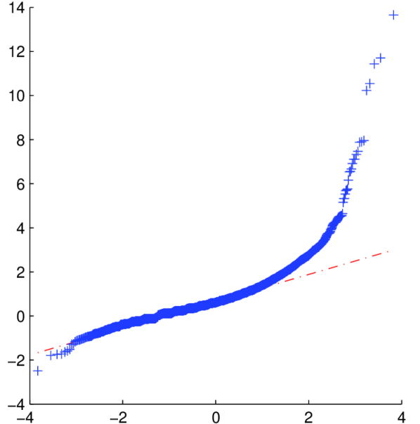
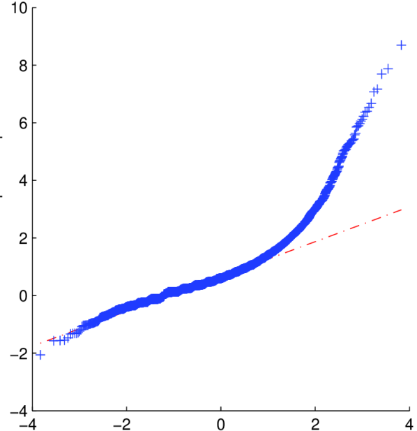
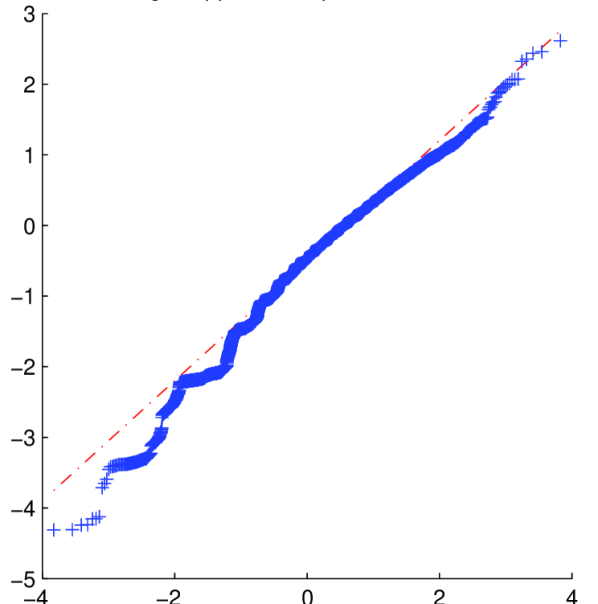
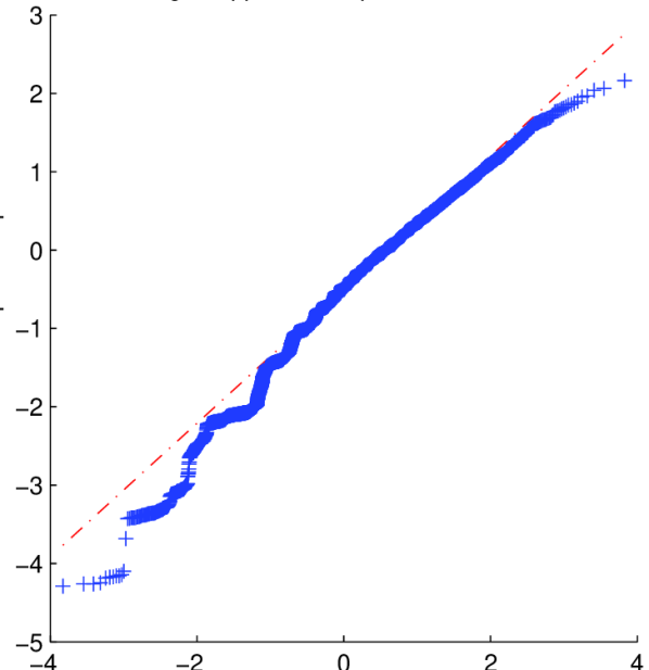
z_min = g_t, if g_t ≤g_t-1 and g_t ≤g_t+1 For financial time series we can regress on the maxima envelope of the absolute returns, shown in figure 1(b). We can also regress on the maxima envelope of the positive returns, the minima envelope of the negative returns, shown in figure 1(d), and then combine the results by using Eq. (6.0.2). The envelopes of financial time series display a log-normal distribution as can be seen in figure 2, and GP regression on envelopes maintains the assumption in Eq. (3). When regressing on the envelope, we are dealing with a lesser number of data points (practically about only one-third of the original data series), and our regression is less affected by the intermediate fluctuation of the data points and we get a relatively smoother estimate of the underlying volatility function.

Figure 2: QQ plots vs the standard normal, standard normal quantiles on the horizontal axis and quantiles of the input sample on the vertical (a) QQ plot of the maxima (upper) envelope. (b) QQ plot of the minima (lower) envelope. (c) QQ plot of the log of the maxima (upper) envelope. (d) QQ plot of the log of the minima (lower) envelope

7 Methodology

Our aim is to evaluate the performance of volatility forecasting approaches based on Gaussian processes, against existing approaches such as GARCH and its commonly used variants. In this section we outline the measures we use for evaluating the forecasting performance. We explain our approach for selecting the best GP kernel for our data, outline the technique we use for hyperparameter inference and our use of Cholesky updating and downdating for updating our covariance matrix at each forecasting step. We also establish a method to ensure that GP forecasts of volatility are an unbiased measure of the underlying variance by comparing the residuals obtained by GARCH versus those obtained from a GP.

7.0.1 Performance Metrics:

The forecasting performance of the prediction technique is evaluated by comparing the underlying volatility $\sigma^{2}$, in this case the proxy for volatility i.e. absolute or squared returns, to the one step ahead forecasts $h$. For evaluating the performance of the different kernels we use four loss functions and two accuracy measures. The loss functions are the same as used by [Hansen2005], and are extensively used in financial volatility forecasting literature for comparison of predicting ability of different models: rCl MSE