Luminosities and infrared excess in Type II and anomalous Cepheids in the Large and Small Magellanic Clouds

Type II and anomalous Cepheids (ACs) are useful distance indicators when there are too few classical Cepheids or when RR Lyrae stars are too faint. Type II and ACs follow a period-luminosity relation as well, but they are less well-studied classes of objects. In this paper we study the sample of 335 Type II and ACs in the Small and Large Magellanic Clouds detected in OGLE-III data. The spectral energy distributions (SEDs) are constructed from photometric data available in the literature and fitted with a dust radiative transfer model, thereby leading to a determination of luminosity and effective temperature. In addition, a subsample of targets is investigated for possible binarity by looking for the light-time travel effect (LITE). Hertzsprung-Russell diagrams (HRD) are constructed and compared to evolutionary tracks and theoretical instability strips (ISs). In agreement with previous suggestions, the BL Her subclass can be explained by the evolution of $\sim$0.5-0.6 $M_{\odot}$ stars evolving off the zero-age horizontal branch and the ACs can be explained by the evolution of $\sim$1.1-2.3 $M_{\odot}$ stars. The evolution of the W Vir subclass is not clear. These objects are at higher luminosities than ACs and evolutionary tracks of $\sim$2.5-4 $M_{\odot}$ stars cross this region in the HRD, but the periods of the W Vir are longer than those of the short period classical Cepheids at these luminosities, which indicates the former have lower masses. A low-mass star experiencing a thermal pulse when the envelope mass is small can make a blue loop into the IS region of the W Vir stars. But the timescale is extremely short, so this is also no explanation for the W Vir as a class. A relation to binarity might be at the origin of the W Vir stars, which has already been explicitly suggested for the peculiar W Vir stars. For $\sim 60\%$ of the RV Tau and $\sim 10\%$ of the W Vir objects an infrared excess is detected from the SED fitting. A recent result is confirmed that stars exist with luminosities below that predicted from single-star evolution, which show a clear infrared excess, and the shape of the excess suggests a connection to binary evolution. The investigation of the LITE effect revealed 20 systems that appear to show periodic variations and may be new binaries, although this study requires follow-up. About 40 stars show significant period changes.

1 Introduction

Type II Cepheids (T2Cs) are pulsating low-mass stars stars that are usually associated with the old Population II (hence the name). They are typically separated into three subgroups according to their pulsation periods, but the exact definition of the dividing periods varies; see Welch (2012). In the OGLE-III samples that we use in this paper, the BL Herculis (BLH) stars have pulsation periods of $1-4$ days, the W Virginis (WVir) $4-20$ days, and the RV Tauris (RVT) $20-70$ days. This classification is based on the sample in the Large and Small Magellanic Clouds (LMC and SMC), as described in Soszyński et al. (2008) and Soszyński et al. (2010b). So far, only fundamental mode (FU) pulsators have been discovered.

Evolutionary modelling of T2Cs has been pioneered by Gingold (1976) and Gingold (1985), who established that T2Cs are low-mass stars ”evolving from the blue horizontal branch (HB) through the instability strip (IS) to the asymptotic giant branch (AGB) for the short-period stars, blue loops off the AGB for the stars of intermediate period, and post-AGB (PAGB) evolution for the longest period” as in Wallerstein (2002). Bono et al. (1997a) came to the conclusion that these should be low-mass ($0.52$ to $0.8\leavevmode\nobreak\ {\mbox{$M_{\odot}$}}$), low-metallicity ([Fe/H] = $-1.3$ to $-2.3$) objects. Wallerstein (2002) remarks that the evolution of $1.0\leavevmode\nobreak\ {\mbox{$M_{\odot}$}}$ star at [Fe/H] = $-1.3$ by Vassiliadis & Wood (1993) closely describes the T2C parameters, in particular the transition from the AGB to PAGB phase, and the occurrence of RVT stars.

Anomalous Cepheids (ACs) are also pulsating stars that overlap in period range with RR Lyrae (RRL) and BLH stars. Although ACs share the IS with RRL and BLH stars, these pulsating stars seem to be stars with higher masses that have evolved to the IS. Anomalous Cepheids pulsate in the fundamental mode (FU) and first overtone (FO) as well.

Looking at the $PL$ relations of different pulsating stars in the LMC and SMC, they definitely form a separate relation distinguishing themselves from RRL, classical Cepheids, and T2Cs. Fiorentino & Monelli (2012) argue that if the ACs were single stars evolving in the Hertzsprung-Russell diagram (HRD), i.e. not resulting from binary interaction, they should be metal-poor stars that do not cross into the classical Cepheid IS, while Caputo et al. (2004) investigated the possibility that they continue to the $PL$ relation of classical Cepheids, which was not substantiated significantly.

Previously, Bono et al. (1997b) and Marconi et al. (2004) have modelled these stars. Bono et al. (1997b) treat the evolutionary status of these stars as if they were evolving from the horizontal branch (HB), but they state that it is hard to distinguish if they have evolved as a single star or as a result of mass transfer in a binary system (Renzini et al., 1977). According to Fiorentino & Monelli (2012), their mean mass is around $1.2\pm 0.2\leavevmode\nobreak\ {\mbox{$M_{\odot}$}}$. Martínez-Vázquez et al. (2016) derive an average mass of $1.5\leavevmode\nobreak\ {\mbox{$M_{\odot}$}}$ for four ACs in Sculptor.

Recently, Kamath et al. (2016) presented a newly discovered class of low-luminosity, dusty, evolved objects in the Magellanic Clouds (MCs). These objects have dust excesses, stellar parameters, and spectral energy distributions (SEDs) similar to those of dusty PAGB stars. However, they have lower luminosities and hence lower masses. Kamath et al. (2016) suggests that these objects have evolved off the red giant branch (RGB) instead of the AGB as a result of binary interaction. Interestingly, many of their post-RGB/AGB candidates are known T2Cs. Their initial search was based on optically visible PAGB stars (or candidates) in the MCs (Kamath et al., 2014, 2015), so we considered that it would be interesting to look specifically for infrared excess starting from a sample of T2Cs. The OGLE-III catalogues (Soszyński et al. (2008), Soszyński et al. (2010b), Soszyński et al. (2010a)) provide us with a unique sample of 335 T2Cs and ACs in the SMC and LMC. In the present paper we determine the luminosity and effective temperature of the T2Cs and ACs by fitting the SEDs and we identify stars with an infrared excess. In addition we look for the light-time travel (LITE) effect in (O-C) diagrams to identify candidate binary systems. In an accompanying paper we will investigate the period-luminosity and period-radius relation of T2Cs and ACs and we will estimate the masses of these objects. In section 2 we introduce the sample of T2Cs and ACs. Section 3 presents the photometric data used to construct the SEDs and the model and procedure to fit it. In section 4 we investigate the LITE effect in selected systems. Section 5 discusses the results, and our conclusions are presented in Section 6.

2 The sample

We used the OGLE-III sample of T2Cs and ACs introduced by Soszyński et al. (2008) and Soszyński et al. (2010b). Soszyński et al. (2008) classify 197 T2Cs, which was updated in 2009 to 203 objects in the online catalogue (64 BLH, 97 WVir, and 42 RVT stars), and 83 ACs (62 FU and 21 FO mode) in the LMC. Soszyński et al. (2010b) classify 43 T2Cs (17 BLH, 17 WVir, and 9 RVT stars), while Soszyński et al. (2010a) identify 6 (candidate) ACs (3 FU and 3 FO mode) in the SMC. Some WVir objects have been labelled as ”peculiar W Virginis” (pWVir) objects, which in most cases is an indication that the pulsating star is in a binary system. This is the sample of 335 stars considered in the paper. The periods are taken from the OGLE catalogues. Specifically for the RVT, which show light curves (LCs) with alternating deep and shallow minima, this implies that the periods refer to the time between consecutive minima (thought to be the true pulsation period), not the time between deep (or shallow) minima. After this work was completed Soszyński et al. (2015a) provided a new catalogue of 250 ACs, 141 in the LMC and 109 in the SMC, based on OGLE-IV data. This larger sample will be considered in a future paper where the analysis presented in this paper will be expanded to classical Cepheids and RR Lyrae stars. The increase of the number of ACs in the SMC is considerable, but all 6 SMC ACs considered here remain in the new catalogue (with the same FU/FO classification). There are some implications for the present paper however. Two of the LMC ACs have been reclassified in the new catalogue: OGLE-LMC-ACEP-022 and -083 are now considered RRL, while OGLE-LMC-T2CEP-114 (formerly a BLH) is considered an AC now. For completeness, the stellar parameters that have been determined and the fits to the SEDs are presented in the Appendices, but the two reclassified RRL are not discussed in the main text and figures, and are excluded in fitting any relations. The numbering scheme remains the same between the OGLE-III and OGLE-IV catalogues for stars 1-83. OGLE-LMC-T2CEP-114 is kept under its OGLE-III name in the present paper but in the figures is plotted as a FU mode AC (OGLE-IV name: OGLE-LMC-ACEP-114). For the SMC the numbering scheme did change with respect to that introduced in the online OGLE-III Variable Stars Database, although all 6 ACs are in fact confirmed with the original FU/FO classification. We keep the OGLE-III numbering in the tables and figures in the present paper. OGLE-SMC-ACEP 01…06 are numbered 32, 41, 57, 62, 68, and 81 in Soszyński et al. (2015a).

3 Constructing and fitting the spectral energy distributions

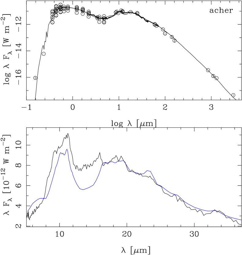
The SEDs were constructed using photometry retrieved mostly, but not exclusively, via the VizieR web interface. In the optical, the mean-magnitudes from OGLE, EROS, and MACHO (when available) are given the highest weight (by assigning a photometric error of 0.01 mag). Additional optical photometry comes from, for example the Magellanic Cloud Photometric Survey (MCPS) (Zaritsky et al. (2002, 2004)), Massey (2002), and Sebo et al. (2002). In the near-infrared (NIR) and longer wavelengths generally no light-curve averaged mean magnitudes exist, but the photometric amplitudes decrease with increasing wavelength and so the effect of the variability on the derived luminosity is lower. There are a fair number of independent measurements available, especially in the NIR, for example DENIS, 2MASS, 2MASS 6X, IRSF (Kato et al., 2007), and the LMC Synoptic Survey (Macri et al., 2015); we also considered NIR photometry from Ciechanowska et al. (2010) and Ripepi et al. (2015) and other publicly available data from the VMC survey (Cioni et al., 2011). At longer wavelengths WISE data were available for the majority of objects (Cutri & et al., 2014). Akari data were available from Ita et al. (2010) and Kato et al. (2012). We retrieved IRAC and sometimes MIPS (multi-epoch) data from the NASA/IPAC Infrared Science Archive. The smallest number of photometric points is 4 (OGLE-LMC-T2CEP-142) and there are seven other stars with 9 or fewer data points. On the other hand there are 10 stars with 40 or more data points. Ninety percent of the 335 Cepheids have between 11 and 36 data points. The SEDs are fitted with More of DUSTY (MoD; Groenewegen (2012)), an extension of the DUSTY radiative transfer code DUSTY (Ivezić et al., 1999). For a given set of photometry, and/or spectra, visibility data, and intensity profiles, as input data the programme determines the best-fitting luminosity ($L$), dust optical depth ($\tau$, at 0.55 $\mu$m), dust temperature at the inner radius ($T_{\rm c}$), and slope of the density profile ($\rho\sim r^{-p}$). Any of these parameters can also be fixed. The SEDs are fitted under the assumption of being representative of a single star. The influence of any unresolved binary on the photometry depends on the luminosity ratio and difference in spectral type and hence the resulting effective temperature and luminosity. Canonical distances of 50.0 and 61.0 kpc are adopted for the LMC and SMC, respectively, corresponding to distance moduli of 18.49 and 18.93, well within the error bars of the current best estimates (de Grijs et al., 2014; de Grijs & Bono, 2015). We decided against fitting the $E(B-V)$ as an additional free parameter and adopted $E(B-V)=0.15$ for all stars. Although this simplification ignores the spatial variation seen in the MCs (e.g. Haschke et al. (2012a, b), Inno et al. (2016)), the effect on the derived luminosity and effective temperature should be small in these stars with SEDs that peak in the NIR. The MARCS model atmospheres are used as input (Gustafsson et al., 2008) for most stars with overall metallicities of [Fe/H]= $-0.50$ and $-0.75$ dex for LMC and SMC stars, respectively. The model grid is available at 250 K intervals for the effective temperature range of interest and we used adjacent model atmospheres to interpolate models at 125 K intervals, which reflects better the accuracy in $T_{\rm eff}$ that can be achieved. A few model atmospheres with temperatures that are hotter than the upper limit of 8000 K available in the MARCS model grid had to be considered and for those we used PHOENIX model atmospheres (Hauschildt et al., 1999). In the end, only one star has a best-fitting temperature above 8000 K. Most stars have no dust and are best represented by a naked star. In those cases the dust optical depth is fixed to a very small number (and $T_{\rm c}$ and $p$ are also fixed to standard values of 1000 K and 2, respectively). For every model atmosphere ($T_{\rm eff}$) a best-fitting luminosity (with its [internal] error) is derived with the corresponding $\chi^{2}$ of the fit. The model with the lowest $\chi^{2}$ then gives the best-fitting effective temperature. Considering models within a certain range above the minimum $\chi^{2}$ then gives the error in the effective temperature and luminosity. For the luminosity this error is added in quadrature to the internal error in $L$. For some stars a better fit is achieved by adding a dust component. The Bayesian information criterion (BIC; see Schwarz (1978)) is used to verify if the lower $\chi^{2}$ that is obviously obtained when adding additional parameters is, in fact, statistically significant. Most of the objects that have an excess are RVT stars, some of which even have a Spitzer IRS spectrum available (see below). It is not our aim to investigate the dust content of RVT stars in the MCs in this paper. As most RVT stars that have an IR excess show SEDs that point to a disc structure rather than an expanding outflow the use of a 1-D code is also limited. For the purpose of the present paper we included a realistic dust component to get a more realistic estimate of the luminosity. The dust component that we used is based on a fit to the SED and dust spectrum of the well-known Galactic RVT star AC Her, which was recently discussed in Hillen et al. (2015). The fit obtained with MoD (using two shells) is shown in Figure 1 and is remarkably good. The dust is a combination of amorphous silicates, corundum, crystalline silicates, and metallic iron, similar to that in Hillen et al. (2015). We used this species in all of the SED fits to the MC stars. The derived luminosities, effective temperatures, and dust optical depth are listed in Table 3 and the fitted SEDs are shown in Figure 12. The stars for which an IRS spectrum is available are explicitly discussed in Section 5.3.

Figure 1: Fit to the SED and ISO SWS spectrum (Sloan et al., 2003) of AC Her, with a two-component wind, illustrating the dust mix that has been used in fitting the stars, which show a clear MIR excess. In the bottom panel the model is scaled to the observed flux in the 20.5-22.5 $\mu$m region to facilitate the comparison of the dust features.

4 A search for binarity

Ten T2C or ACs in the present sample have been identified by the OGLE team to be in eclipsing binary systems. We searched for additional candidate binary systems by investigating the presence of the light-travel time effect or light-time effect (LITE) (Irwin, 1952) in so-called observed minus calculated (O-C) diagrams. Traditionally, the (O-C) diagram is constructed from timing measurements of, typically, maximum light and plotted versus time. Here, we considered and implemented the method outlined in Hajdu et al. (2015), which uses a template LC constructed from the data to determine the (O-C) values. This method is extremely well suited in the case of the long time series available in the OGLE database, where it is impractical to determine individual times of maximum, but where exquisite phased LCs can be constructed. Details are given in Appendix C but in essence the method is as follows:

• A Fourier series is fitted to part of the data to define the template LC. This also defines the reference epoch and pulsation period relative to which the (O-C) diagram is constructed.

• Sections of, typically, 50, consecutive data points are taken and fitted to the template LC and from that the (O-C) value is determined. As an extension to the method proposed by Hajdu et al. (2015) we consider the fact that the observed LC might show amplitude modulations and therfore allow for a possible scaling of the Fourier amplitudes to determine the best fit.

The derived (O-C) diagram might diagnose several physical effects (e.g. see Sterken (2005)) but the most relevant here are a change of the pulsation period with time (resulting in a parabolic shape) and/or the presence of a binary. In the numerical code we fit a function of the form

$$(O-C)(t)=c_{0}+c_{1}t+c_{2}t^{2}+c_{3}t^{3}+...$$ (1)

$$\hskip 85.35826pt...+(a\sin i)\,\frac{1-e^{2}}{1+e\cos(\nu)}\,\sin(\nu+\omega),$$ (2)

where $a$ is the semi-major axis, $i$ is the inclination, $e$ is the eccentricity, and $\omega$ is the argument of the periastron. The true anomaly $\nu$ is a function of the time $t$, the orbital period $P_{\rm orb}$, the time of periastron passage $T_{\rm peri}$, and $e$. All parameters of the model ($c_{0},c_{1},c_{2},c_{3}$, $P_{\rm orb}$, $T_{\rm peri}$, $a\sin i$, $e$, $\omega$) can be fitted or fixed. Since the procedure is time consuming as it requires manual supervision not all objects were investigated. In total, we considered 133 systems. These were the systems classified by OGLE to show eclipsing or ellipsoidal variations, the pWVir stars that have been suggested to be in binary systems, and stars that showed unusual scatter in the rising branch of the published phased LC that hints at changes in period or binarity. In Section 5.4 we discuss candidate binary systems in more detail. In Appendix C we additionally present systems that appear to show significant changes in period, and list, for reference, the remainder of the sources for which the data are inconclusive or that do not show any significant variations in the (O-C) diagram.

In all cases it will be essential to reinvestigate the results when the OGLE-IV data become available, which will extend the time series, allowing us to improve on these findings.

5 Results and discussion

Figure 2: Plot of observed $I,(V-I)$ CMD. Stars in the SMC are plotted in red and are shifted by $-0.432$ mag in $I$ to account for the difference in adopted distance (50 vs. 61 kpc). For the pWVir object OGLE-LMC-T2CEP-098 (MACHO 6.6454.5), a known eclipsing system (Alcock et al., 2002), the location of the two components is indicated by the dark blue lines. The pulsating star is the fainter, redder object (see text). Stars with an IR excess are denoted by a green plus sign. Stars that show eclipsing or ellipsoidal variations according to OGLE are denoted by a blue cross. Some stars are labelled by their identifier.

5.1 Hertzsprung-Russell diagram

Figure 3: Plot of physical Hertzsprung-Russell diagram. Stars in the SMC are plotted in red. Stars with an IR excess are indicated by a green plus sign. Stars that show eclipsing or ellipsoidal variations according to OGLE are indicated by a blue cross. The tracks plotted with $\times$ are the lowest initial mass tracks of Vassiliadis & Wood (1993) for the LMC ($0.945\leavevmode\nobreak\ {\mbox{$M_{\odot}$}}$), and SMC ($0.89\leavevmode\nobreak\ {\mbox{$M_{\odot}$}}$, in red). The final masses are $0.555$ and $0.558\leavevmode\nobreak\ {\mbox{$M_{\odot}$}}$, respectively. The tracks plotted with a $\ast$ are the lowest initial mass tracks of Miller Bertolami (2016) for a metallicity of $Z=0.01$ (1.0 $M_{\odot}$, current mass 0.534 $M_{\odot}$), and $Z=0.001$ (0.9 $M_{\odot}$, current mass 0.536 $M_{\odot}$, in red). In both tracks every tick marked represents 500 years of evolution. The blue and red edge of the fundamental mode IS of BLH (between $\log L\sim 1.81-2.1$, for a mass of 0.65 $M_{\odot}$) and FU ACs (between $\log L\sim 1.77-2.4$) are indicated by the solid line (see text). The vertical dotted lines indicate the location of most of the variables at higher luminosity (see text). Some stars are labelled by their identifier.

Figure 4: Histogram of the distribution over luminosity. In the top panel the black, red, and blue histograms represent all the SMC, and LMC objects, respectively. The latter two are slightly offset by $\pm$0.01 in $\log L$ for clarity. The bottom panel shows the distributions for SMC and LMC objects according to type: BLH (black), ACs (light blue), (p)WVir (red), and RVT (dark blue). The histograms are offset by $\pm$0.01 in $\log L$ for clarity.

Figure 5: As Figure 3 but only for the BLH objects. The blue and red edge of the fundamental mode IS of BLH (between $\log L\sim 1.81-2.1$, for a mass of 0.65 $M_{\odot}$) are indicated by the solid line (Di Criscienzo et al., 2007). The dashed lines indicate the location of the first overtone blue edge and fundamental mode red edge of RR Lyrae (see text). PARSEC horizontal branch models (Bressan et al., 2012) are plotted in light blue ($Z=0.001$), magenta ($Z=0.004$), and yellow ($Z=0.008$) for, respectively, 0.515, 0.56, 0.62 $M_{\odot}$ (decreasing in luminosity), 0.505, 0.53, 0.57 $M_{\odot}$, and 0.50, 0.52, 0.57 $M_{\odot}$ (see text). A point is plotted for every 1 Myr of evolution.

Figure 6: As Figure 3 but only for the AC objects. The fundamental mode (solid line) and first overtone (dashed line) blue and red edge of the IS of AC are indicated (Fiorentino et al., 2006). Tracks from the BaSTI database (Pietrinferni et al., 2004) are plotted in light blue ($Z=0.0001$), magenta ($Z=0.0003$), yellow ($Z=0.0006$), brown ($Z=0.001$), green ($Z=0.002$) for stars of 1.1 $M_{\odot}$ (1 model, bluest extension near $\log L\sim 1.9$), 1.5 $M_{\odot}$ (2 models, bluest extension near $\log L\sim 2.1$), 1.9 $M_{\odot}$ (1 model, bluest extension near $\log L\sim 2.2$), and 2.3 $M_{\odot}$ (3 models, bluest extension between $\log L=2.25-2.45$). A point is plotted for every 1 Myr of evolution.

Figure 7: As Figure 3 but only for the (p)WVir. For reference, the fundamental mode (solid line) and first overtone (dashed line) blue (for $Z=0.004$) and red edge (for $Z=0.008$) of the IS of classical Cepheids are indicated Bono et al. (2000). Tracks from the BaSTI database (Pietrinferni et al., 2004) are plotted in light blue ($Z=0.001$), magnenta ($Z=0.002$), yellow ($Z=0.004$), and brown ($Z=0.008$) for stars with initial masses of 2.5 $M_{\odot}$ (2 models, bluest extension between $\log L=2.2-2.4$), 3.0 $M_{\odot}$ (3 models, bluest extension between $\log L=2.35-2.8$), and 4.0 $M_{\odot}$ (2 models, bluest extension between $\log L=3.0-3.2$). A point is plotted for every 1 Myr of evolution. The dark blue track represents the evolutionary track (Miller Bertolami, private communication) of a star with 0.60 $M_{\odot}$ at the ZAHB that evolved through the AGB and experiences a TP, which results in the star crossing the IS. The evolution in that region is very fast. Each points represents 10 years of evolution.

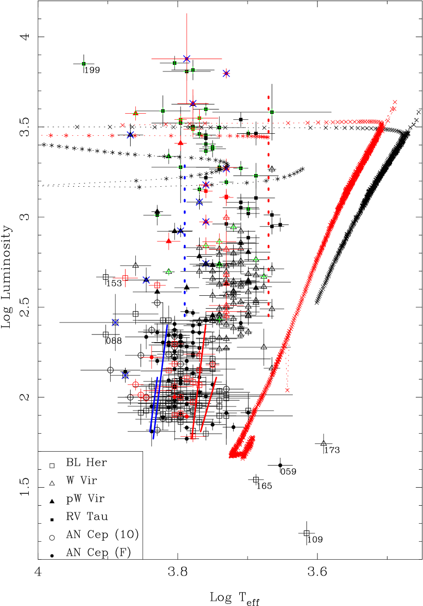
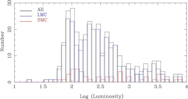
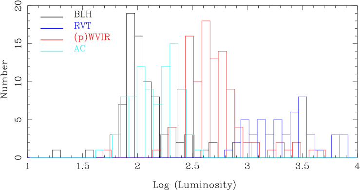
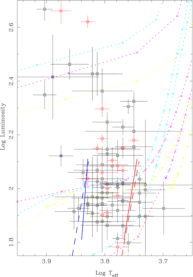
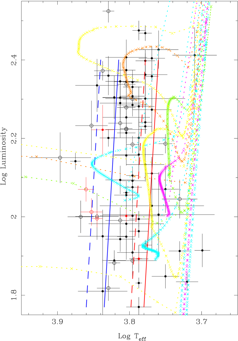
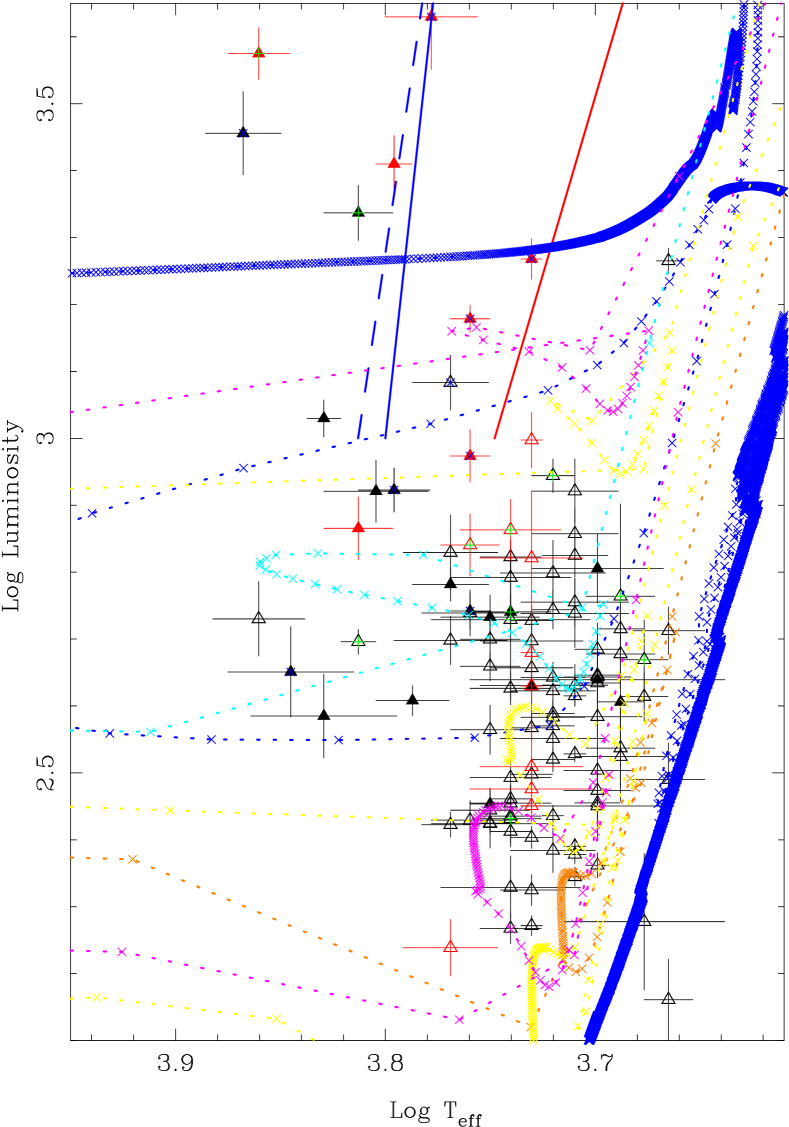
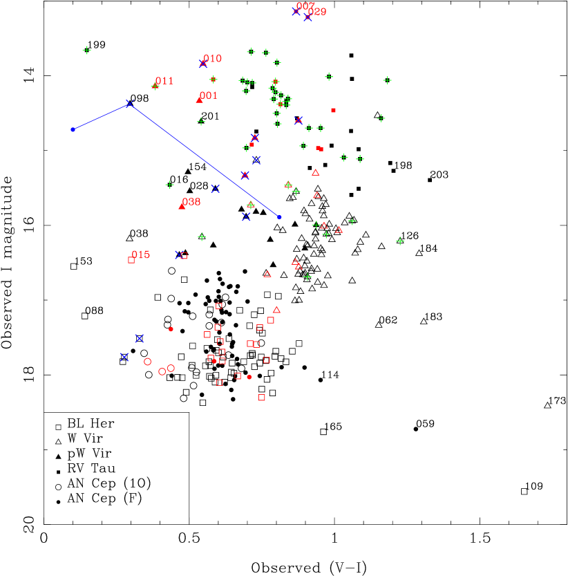
Figure 2 shows the observed $I,(V-I)$ colour-magnitude diagram (CMD) essentially combining Figure 2 in Soszyński et al. (2008) and Figure 2 in Soszyński et al. (2010b) into one. They did not comment on the apparent outliers at the time.

LMC-T2CEP-098 is an interesting case. It is classified as a pWVir and is an eclipsing binary (EB). It has been analysed by Alcock et al. (2002) who derived the magnitudes of the components. These are also plotted in Figure 2 and illustrate how binarity can influence the appearance on the CMD. The pulsating star is located close to the bulk of the WVir stars, while its bright non-pulsating component makes the system appear rather blue.

LMC-T2CEP-088 and -153 (near $I\sim 17,(V-I)=0.1$) are indicated as ”blended” by OGLE, which probably explains their blue colour. The blue colour of LMC-T2CEP-199 (near $I\sim 14$) is probably real. It has the hottest effective temperature (8600 K) based on the fits to the SED of all stars and it has been classified as a B2III object (see below). The four stars that are fainter than the other stars are not remarkable in any way (in terms of the SED or their LC), which would explain their position in the CMD. An anonymous referee for this paper suggested that three objects (T2CEP-165, -173, ACEP-059) are in the direction of the Tarantula Nebula (30 Dor) and that high reddening could play a role. This is certainly possible as the distance from -165 to 30 Dor is about 20′ and that of the other two objects is about 45′. However there are a few T2Cs and ACs located even closer than 20′ and many objects within 45′ that are not outliers.

Figure 3 shows the physical Hertzsprung-Russell diagram (HRD). The same morphology as in the $I,(V-I)$ CMD is seen. We treated stars as single stars in the SED fitting so that binaries would appear more luminous and hotter (assuming the companion is an unevolved object) than the parameters the pulsating component would have. The evolutionary tracks from Vassiliadis & Wood (1993) of a 0.945 $M_{\odot}$ (for LMC abundance) and 0.89 $M_{\odot}$ (for SMC abundance, in red) initial mass star are plotted for reference as the crosses. Recently, Miller Bertolami (2016) published new PAGB tracks. The lowest available initial mass tracks for a metallicity of $Z=0.01$ (1.0 $M_{\odot}$, current mass 0.534 $M_{\odot}$) and $Z=0.001$ (0.9 $M_{\odot}$, current mass 0.536 $M_{\odot}$, plotted in red) are plotted with a $\ast$. For both sets every tick mark represents 500 years of stellar evolution. The important thing to note is that stars with IR excess (denoted by the green plus sign) occur at luminosities below those allowed for by single-star evolutionary tracks, as found by Kamath et al. (2016).

The IS of the BLH and ACs are indicated in Fig. 3 and are further explored in Figs. 5 and 6, which show the HRD for these classes of objects in detail. At higher luminosities, covering the WVir (including the pWVir objects), and the lower luminosity RVT stars, an IS is drawn by eye in Fig. 3 that covers most variables. The red edge is drawn at $\log T_{\rm eff}=3.67$ ($T_{\rm eff}=4680$ K), the blue edge at $\log T_{\rm eff}=3.79$ ($T_{\rm eff}=6160$ K). The red edge seems to cover the variables for all luminosities in the present sample, for the blue edge a simple constant effective temperature seems to be a good approximation only up to $\log L\sim 3.3$.

Figure 4 shows the projection of the HRD onto the luminosity axis. The luminosity distribution is qualitatively similar to that of T2C in globular clusters shown in Gingold (1985) with a minimum in the distribution around $\log L\sim 2.2$ (but at slightly larger luminosity in the SMC, although there are fewer stars).

Figure 5 shows the blue and red edge of the FU IS of BLH (Di Criscienzo et al., 2007) (between $\log L\sim 1.81-2.1$) for a mass of 0.65 $M_{\odot}$. The IS of the BLH depends little on mass; changing it to 0.55 $M_{\odot}$ would make the IS bluer by a very small amount of $\Delta\log T_{\rm eff}=0.009$. The BLH models were calculated for metallicities between $Z=0.0001$ and $0.004$ and the IS does not appear to depend on metallicity within this range (Di Criscienzo et al., 2007). The observations are in good agreement with the theoretical blue edge, but there are some stars that are cooler by up to 500 K than the theoretical red edge. For comparison, the range in effective temperature covered by similar mass RR Lyrae stars is illustrated by the FU blue edge and the FU red edge based on Marconi et al. (2015) for a metallicity of [Fe/H]= $-1.5$. The figure also shows selected horizontal branch models from the PARSEC tracks (Bressan et al., 2012) that encompass the observations. The most luminous stars could be explained by the lowest masses (0.50-0.515 $M_{\odot}$, depending on metallicity), while the bulk of the stars would have masses in the range 0.52-0.56 $M_{\odot}$.

Figure 6 shows the FU (solid line) and FO (dashed line) blue and red edge of ACs (Fiorentino et al., 2006). The models, calculated for $Z=0.0001$, show a remarkable agreement with the observations. The overtone pulsators are preferentially located at hotter temperatures consistent with the IS. With two exceptions the first overtone pulsators have temperatures between 5625 and 7375 K with a median of 6500 K and with two exceptions. The FU pulsators have temperatures between 5000 and 7000 K with a median of 6250 K. Figure 6 also includes evolutionary tracks from the BaSTI library (Pietrinferni et al., 2004) for masses and metallicities that cover the region in the HRD where the ACs are found. The lower luminosites would be explained by low-mass ($\sim 1.1\leavevmode\nobreak\ \mbox{$M_{\odot}$}$) low-metallicity ($Z=0.0001$) stars, the upper luminosity range by stars of $\sim$ 2.3 $M_{\odot}$ at 10 times that metallicity. The few ACs observed at the lowest luminosities ($\log L\sim 1.8\leavevmode\nobreak\ \mbox{$L_{\odot}$}$) could be explained by the fast evolution of such stars crossing the IS on their way to the base of the RGB.

Figure 7 shows the WVir (including pWVir) objects, which are located at relatively high luminosity. The pWVir objects are plotted as filled symbols and most of these are hotter than the bulk of the WVir objects. For reference, the IS of classical Cepheids is shown (Bono et al., 2000). It shows that the (p)WVir are not simply the extension of classical Cepheids to lower masses, even though evolutionary tracks can be found that cover the observed location in the HRD.

The figure shows BaSTI tracks (Pietrinferni et al., 2004) for selected models with metallicities between $Z=0.001$ and $Z=0.008$ (see caption for details) for stars of 2.5, 3.0, and 4.0 $M_{\odot}$.

However the WVir objects as a class cannot be counterparts of such stars. The FU pulsation period of classical Cepheids of 5 $M_{\odot}$ (the lowest mass considered in Bono et al. (2000)) is of order 5 days, while the typical period of the bulk of the WVir with $\log L=2.8-3$ and $\log T_{\rm eff}<3.78$ is 15 days. Even a rough application of the period-luminosity-mass relation of classical Cepheids by Bono et al. (2000) indicates that the bulk of the (p)WVir objects should have masses of order 1 $M_{\odot}$ (near $\log L=3$) or less (at lower luminosities). However, single stars of 1 $M_{\odot}$ or lower do not cross the IS at these luminosities.

Another argument are the evolutionary timescales. Along the tracks a point is plotted for every million years. The 4 $M_{\odot}$ star that loops in to the classical Cepheid IS spends a few million years there. In the OGLE-IV catalogues of SMC and LMC (Soszyński et al., 2015b) about 4100 of the 5100 FU mode classical Cepheids have periods below five days, while there are only about 110 WVir in our sample, which, according to the tracks plotted in Fig. 7 spend many millions of years in the IS. This calculation is very rough, ignoring the details of the star formation rate, the initial mass function, and incompleteness, but the mismatch is evident.

One scenario to explain the WVir stars is that these stars experience a thermal pulse on the AGB when the envelope mass is low enough for the star to make an excursion to lower luminosities and higher effective temperatures (Gingold, 1976, 1985). A modern view on this scenario is also presented in Fig. 7. The evolutionary track is shown of a star of 0.60 $M_{\odot}$ (and [Fe/H]$=-1$) evolving off the zero-age horizontal branch (ZAHB) (based on the Miller Bertolami (2016) models, private communication). This example was picked to show that these excursions are possible. The TP occurs when the envelope mass is 0.0073 $M_{\odot}$. The star ends as a 0.522 $M_{\odot}$ white dwarf which, through the initial final mass relation (Gesicki et al., 2014), suggests an initial mass of $\stackrel{{\scriptstyle<}}{{\sim}}$1.25 $M_{\odot}$. The evolution is extremely fast however, the time spent in the IS region is only of order 100 years. This shows that this scenario may apply to very rare individual cases of WVir stars, which would then show very large period changes, but cannot explain the WVir as a class.

In conclusion, the evolutionary status of these stars remains unclear. As single-star evolution appears not to be able to explain the WVir, the binary hypothesis must be considered in more detail, as has been suggested specifically for the pWVir class.

5.2 Comparison to the literature

Table 1: Stellar parameters from the literature for the sample.

Name	$T_{\rm eff}$	$\log g$	[Fe/H]	$L$	Classification	$M$	Ref.	OGLE Name	$T_{\rm eff}$	$L$
	(K)			($L_{\odot}$)		($M_{\odot}$)			(K)	($L_{\odot}$)
SMC
J005107.19-734133.3	5767	0.72	-1.56	3465	P-RGB Disc	0.43	1	T2CEP-018 (RVT)	5875 $\pm$ 375	3539 $\pm$ 166
LMC
MACHO 47.2496.8	4900	0.0	-1.5	5000	-	-	4	T2CEP-015 (RVT)	5000 $\pm$ 125	2910 $\pm$ 053
J050304.95-684024.7	5586	0.5	-2.3	3251	P-RGB Disc	0.44	2	T2CEP-029 (RVT)	5750 $\pm$ 188	2851 $\pm$ 079
J050738.94-682005.9	5420	1.5	-1.0	859	P-RGB Disc	0.37	2	T2CEP-046 (WVIR)	5250 $\pm$ 125	0879 $\pm$ 021
J051418.09-691234.9	6112	0.5	-1.6	6667	P-AGB Disc	0.57	2	T2CEP-067 (RVT)	6125 $\pm$ 500	6429 $\pm$ 305
(idem)	5750	0.5	-2.0	5000 $\pm$ 500	-	-	3	T2CEP-067 (RVT)	…	….
J051845.47-690321.8	5860	1.5	-0.8	4001	YSO	-	2	T2CEP-091 (RVT)	6625 $\pm$ 625	3880 $\pm$ 319
J052519.48-705410.0	8117	1.0	-0.5	3219	P-AGB Disc	0.58	2	T2CEP-119 (RVT)	6250 $\pm$ 625	3325 $\pm$ 290
J053150.9-691146	6000	0.5	-2.5	4000 $\pm$ 500	-	-	3	T2CEP-147 (RVT)	6375 $\pm$ 312	7160 $\pm$ 259
(idem)	6000	0.5	-2.5	-	-	-	5	T2CEP-147 (RVT)	…	….
J053254.5-693513	6250	1.0	-1.5	4200 $\pm$ 500	-	-	3	T2CEP-149 (RVT)	5750 $\pm$ 250	2741 $\pm$ 117
J054000.5-694214	5103	1.5	-1.9	4200 $\pm$ 500	-	-	3	T2CEP-174 (RVT)	6000 $\pm$ 438	6549 $\pm$ 342
J054312.86-683357.1	5103	1.5	-1.9	3085	YSO	-	2	T2CEP-180 (RVT)	5500 $\pm$ 500	3139 $\pm$ 182
J055122.52-695351.4	6237	1.5	-2.5	3780	P-AGB Disc	0.56	2	T2CEP-191 (RVT)	5750 $\pm$ 250	3969 $\pm$ 127

(1) Kamath et al. (2014); (2) Kamath et al. (2015); (3) Gielen et al. (2009); (4) Reyniers et al. (2007), also see Pollard & Lloyd Evans (2000); (5) Reyniers & van Winckel (2007).

Some of the stars in our sample have been analysed previously using high-resolution spectroscopy and Table 9 contains the stellar parameters derived in the literature. Columns 1-5 list the name, effective temperature, gravity, and total luminosity, with an error bar when explicitly given, from the literature. For the stars in common with Kamath et al. (2014, 2015) the next two columns show their classification: two stars are classified as young stellar objects (YSO), three stars as post-RGB, and three as PAGB stars, and all six show disc-like SED (contrary to shell-like), and current mass. The last three columns give the OGLE name, and the effective temperature and luminosity derived in the present paper (from Table 3).

In most cases the agreement is very good (within our 2$\sigma$ error bars), keeping in mind as well that the spectra were taken during one phase in the pulsation cycle while the stellar parameters derived here are based on all available photometry and so should represent the star at mean light.

The most discrepant values are the luminosity of LMC-T2CEP-015 and the effective temperature of LMC-T2CEP-119. There are no obvious reasons for the discrepancies. The fits to both SEDs are good. Interestingly, both stars have an IR excess (see Sect. 5.3), which may have influenced the analysis in Kamath et al. in some way. Reyniers et al. (2007) fitted the SED of LMC-T2CEP-015 but only had photometry up to the $K$-band available, not noticing the excess emission. From fitting the SED, van Aarle et al. (2011) find $L=3080\pm 150$ $L_{\odot}$, and $T_{\rm eff}=4750\pm 250$ K in good agreement with our determination and quote a spectral type G2-8(R)Ibe, which also points to a temperature around 5000 K. For LMC-T2CEP-119 van Aarle et al. (2011) give a spectral type of G0Ib suggesting a temperature slightly below 6000 K, which is closer to our determination than the high value by Kamath et al.

5.3 Far-infrared excess, and the RV Tau phenomenon

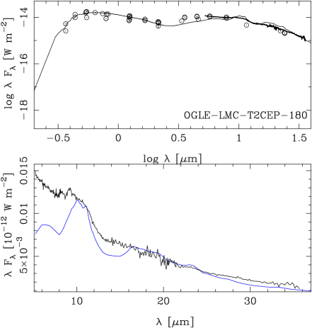
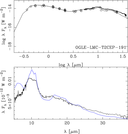
For 10 stars Spitzer Space telescope IRS spectra (Houck et al., 2004) are available, which are all in the LMC and are all classified as RV Tau stars. The spectra have been discussed in detail in Gielen et al. (2011) in the context of silicate features in Galactic and extragalactic PAGB stars. Figure 8 shows the fitted SEDs of the RVT stars with their IRS spectra. The spectrum was not used in the SED fitting; the spectra are overplotted on top of the best model fit to the overall SED. In the bottom panel the model is scaled to the observed flux in the 20.5-22.5 $\mu$m region to facilitate the comparison of the dust features.

It is not the aim of this paper to discuss in detail the spectral features of the RVT stars in the MCs (see Gielen et al., 2011). In most cases the spectral shapes are well fitted and very similar to the template of the Galactic RV Tau star AC Her. If there are larger differences then these are always in the sense that the silicate feature appears weaker w.r.t. the dust continuum (stars 067, 104, 174, 180).

Figure 8: Fits to the SEDs of the RV Tau stars that have an IRS spectrum. In the bottom panel the model is scaled to the observed flux in the 20.5-22.5 $\mu$m region to facilitate the comparison of the dust features.

Figure 8: Continued

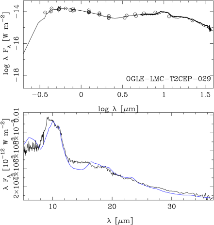
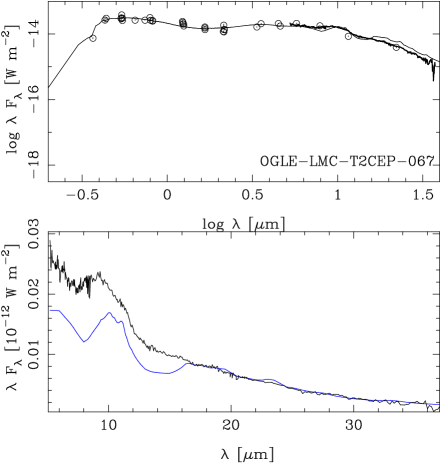
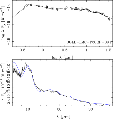
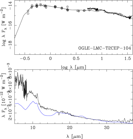
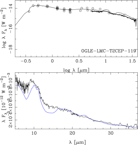
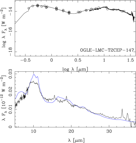
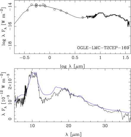
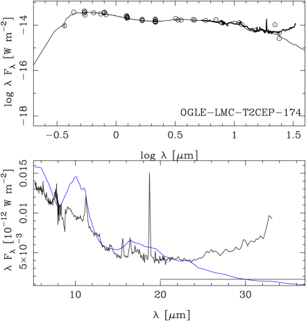
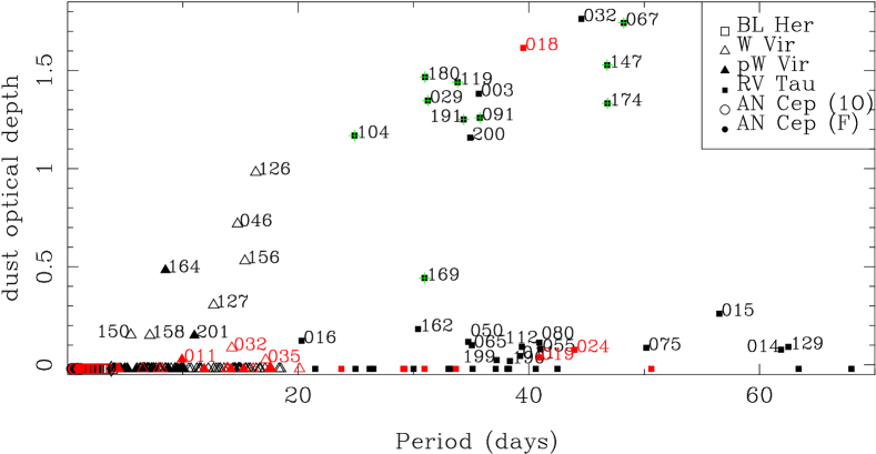
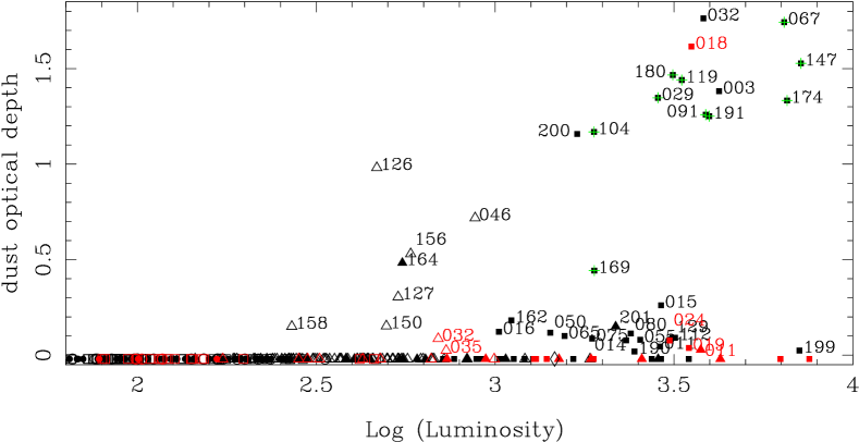
There are more stars that show (weak) excess IR emission than the 10 for which IRS spectra are available. The results are summarised in Fig. 9, where the derived dust optical depth is plotted against period and luminosity with more detailed information available in the Appendices. In some cases it is difficult to exclude excess emission definitively. Table 3 includes 4 objects for which the WISE W4 filter is unreliable, but where the W3 filter lies above the model atmosphere. These stars are marked (”W3 excess”). If the excess were real it would imply very low optical depths and these sources could be examples of where the dust shell has expanded away from the star, contrary to most SEDs of stars with excess emission that point to hot dust and a disc structure. Another four objects are marked (”IR excess?”), where there could possibly be weak IR excess; one of these is the RVT object OGLE-LMC-T2CEP-025, which has the longest period in the sample at 68 days.

Infrared excess is absent (or undetectable) in AC (0:76) and BL Her (0:81) objects and present in $\sim 10\%$ of the W Vir objects (3:24 pWVir, and 8:90 WVir). In RVT the phenomenon is common with 30:52 objects showing detectable emission (plus 3 possible). Of the 41 stars with detectable IR emission only 6 are located in the SMC.

The SEDs of PAGB and RVT objects are typically divided between sources showing hot dust, which are interpreted as dust in a circumbinary system, and those showing cold dust, which are interpreted as dust in an expanding shell; see for example the recent work by Gezer et al. (2015) (their Figure 2) and references therein. This distinction is also seen in Fig. 9. All objects with a derived optical depth above unity show SEDs characteristic of disc sources. For optical depths $\stackrel{{\scriptstyle<}}{{\sim}}$ 0.2 the SEDs are all consistent with an expanding shell model. For the half dozen stars with intermediate optical depths one could argue either way.

As stated above, the disc sources are thought to be binary objects. The OGLE catalogues identify additional eclipsing variability in the LCs of 10 of the stars in the sample (marked ”EB” in Table 3, one of which is an RVT star), but excess emission is detected in none of them.

Figure 9: Dependence of the derived dust optical depth on pulsation period and $\log L$. Stars in the SMC are plotted in red. Stars with an IRS spectrum are indicated by a green plus sign. Stars with a detectable IR excess are labelled by their identifier.

5.4 Candidate binary T2C

Table 2 lists the systems where our investigation suggested a possible binary system. The (phased) LC and the (O-C) diagrams and model fits are shown in Figure 4. The Table lists the binary period, time of periastron, $a\sin i$, and the change in period, $\dot{P}$. Pulsation type and period are repeated from Table 3. The last column adds some remarks. The eccentricity was fixed to zero, except in one case, where the data were good enough and required a non-zero eccentricity. The LITE could only be established in one known EB, and only marginally in two others. For LMC-T2CEP-021 the derived binary period of 172 days is in good agreement with the period of 174.8 days that was photometrically derived by the OGLE team.

Most of the candidate binary systems hosts are (p)WVir stars. As mentioned in Sect. 4 the main criterion for investigating a possible LITE was unusual scatter in the raising branch of the phased LC. This was not the case for the BLH and ACs, and only 13 out of 170 such objects were investigated for the LITE with only 2 candidate binaries (and 2 known BLH where the LITE was not found). For the (p)WVir and RVT about half of the stars in the sample were investigated for the LITE with only a few candidates among the RVT, and about 1/3 among (p)WVir. On the other hand, one RVT and 5 (p)WVir in known EB systems did not show the LITE using the present data.

There is no correlation between candidate binary systems and infrared excess. Only 3 of the 23 candidates also shows IR excess in their SEDs.

Table 2: T2C candidate binaries from the LITE.

Name	$P_{\rm bin}$	$T_{\rm peri}$	$a\sin i$	$\dot{P}$	Type	Period	Remarks
	(d)	(JD-2450000)	(AU)	(s/yr)		(d)
LMC-ACEP-050	2468 $\pm$ 68	4770 $\pm$ 30	5.33 $\pm$ 0.37	$-1.06\pm 0.06$	ANCep	1.0
LMC-T2CEP-011	1657 $\pm$ 255	4252 $\pm$ 133	500. $\pm$ 88.	0 (fixed)	RVTau	39.3	IR excess
LMC-T2CEP-021	172 $\pm$ 4.2	3447 $\pm$ 12	57. $\pm$ 27.	$505\pm 108$	pWVir	9.8	known EB
LMC-T2CEP-033	2643 $\pm$ 92	5775 $\pm$ 46	90. $\pm$ 10.	0 (fixed)	pWVir	9.4
LMC-T2CEP-040	3552 $\pm$ 2226	7207 $\pm$ 51	166. $\pm$ 234.	0 (fixed)	pWVir	9.6	marginal LITE
LMC-T2CEP-044	2784 $\pm$ 246	5047 $\pm$ 82	163. $\pm$ 15.	$233\pm 62$	WVir	13.3
LMC-T2CEP-062	2622 $\pm$ 140	2446 $\pm$ 47	56.0 $\pm$ 5.1	$-31.2\pm 6.5$	WVir	6.0
LMC-T2CEP-079	1568 $\pm$ 109	5688 $\pm$ 64	64.4 $\pm$ 6.4	$631\pm 58$	WVir	14.9
LMC-T2CEP-087	2951 $\pm$ 85	6669 $\pm$ 79	41. $\pm$ 12.	0 (fixed)	WVir	5.2	$e=0.74^{+0.23}_{-0.17}$, $\omega=18\pm 12\deg$
LMC-T2CEP-097	2221 $\pm$ 81	4741 $\pm$ 48	90. $\pm$ 12.	$-107\pm 21$	WVir	10.5
LMC-T2CEP-098	397 (fixed)	2970 $\pm$ 22	8.7 $\pm$ 2.6	0 (fixed)	pWVir	5.0	known EB, marginal LITE
LMC-T2CEP-100	1905 $\pm$ 171	4114 $\pm$ 82	31.7 $\pm$ 4.5	$-31\pm 15$	WVir	7.4	Fit for JD $>$1600,
							Very different period before
LMC-T2CEP-106	1617 $\pm$ 38	3819 $\pm$ 30	39.3 $\pm$ 6.1	0 (fixed)	WVir	6.7
LMC-T2CEP-127	3352 $\pm$ 319	7068 $\pm$ 82	408 $\pm$ 71	$-884\pm 230$	WVir	12.7	IR excess
LMC-T2CEP-132	2632 $\pm$ 102	6576 $\pm$ 83	94 $\pm$ 11	0 (fixed)	pWVir	10.0	amplitude variations
LMC-T2CEP-137	2417 $\pm$ 84	7406 $\pm$ 116	60.6 $\pm$ 6.6	$24.7\pm 7.1$	WVir	6.4
LMC-T2CEP-168	1668 $\pm$ 171	6016 $\pm$ 120	42.5 $\pm$ 5.5	$145\pm 69$	WVir	15.7
LMC-T2CEP-172	1983 $\pm$ 101	5379 $\pm$ 69	69.8 $\pm$ 10.8	$78\pm 29$	WVir	11.2
LMC-T2CEP-177	2060 $\pm$ 68	6229 $\pm$ 37	83.8 $\pm$ 2.8	0 (fixed)	WVir	15.0
SMC-T2CEP-001	2019 $\pm$ 84	5029 $\pm$ 41	85.1 $\pm$ 11.5	0 (fixed)	pWVir	11.9
SMC-T2CEP-018	1404 $\pm$ 61	5554 $\pm$ 48	368 $\pm$ 80	0 (fixed)	RVTau	39.5	IR excess
SMC-T2CEP-029	609 (fixed)	3569 $\pm$ 46	25 $\pm$ 18	$-960\pm 75$	RVTau	33.7	known EB, marginal LITE
SMC-T2CEP-030	2354 $\pm$ 226	5929 $\pm$ 103	5.02 $\pm$ 0.93	$1.6\pm 0.9$	BLHer	3.9

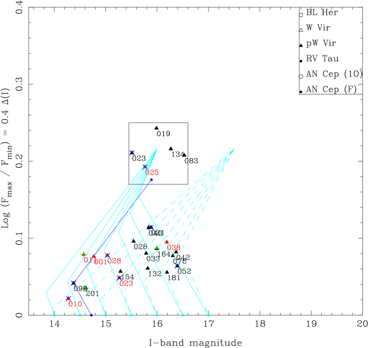
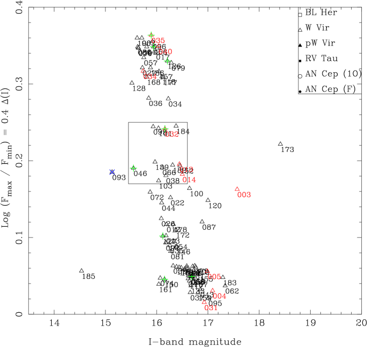
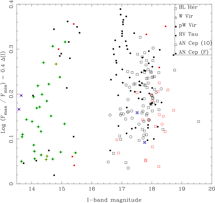
Another way to investigate binarity is to look for unusually low pulsation amplitudes. If a pulsating star is in a physical binary with a (assumed to be non-pulsating) secondary, the amplitude of the system is smaller. Also the magnitude and colour are affected, which was already illustrated in Fig. 2 for the system pWVir object LMC-T2CEP-098.

In Fig. 10 the logarithm of the ratio between the flux at maximum and minimum light (or $0.4\times$ the peak-to-peak amplitude) is plotted against $I$ magnitudes for the pWVir (top), WVir (middle), and all other objects (bottom panel). For LMC-T2CEP-098 the position of the two components and the position of the system as it is observed are shown. The pulsating component is located in a region occupied by WVir stars. Interestingly, some other objects classified as pWVir (those enclosed in the box) show amplitudes and magnitudes that are comparable to WVir stars. The unusual location of LMC-T2CEP-185 can be explained by the fact that it is listed as a blended object. The light blue lines indicate the locations of hypothetical systems consisting of a 16.0 and 17.5 mag pulsating variable with a peak-to-peak amplitude of 0.54 mag and a non-pulsating companion of various magnitudes. The group of small amplitudes pWVir can indeed be explained by such binary systems.

Figure 10: Logarithm of the ratio between the flux at maximum and minimum light, i.e. $0.4\times$ the peak-to-peak amplitude, vs. mean $I$-band magnitudes for the pWVir (top), WVir (middle), and all other (bottom) objects. Stars with an IR excess are indicated by a green plus sign. Stars that show eclipsing or ellipsoidal variations according to OGLE are indicated by a blue cross. For the pWVir object -098 (MACHO 6.6454.5), a known eclipsing system, the location of the two components is also indicated by dark blue lines. The light blue lines indicate the location of two hypothetical binary systems, consisting of a pulsating component with a fixed amplitude and an increasingly fainter non-pulsating component. The pWVir stars that appear like normal WVir are enclosed by a box that is repeated in the middle panel.

5.5 Period changes

The analysis of the LCs to identify the LITE also includes a term that takes into account any period change. Table 2 lists $\dot{P}$ (can be zero or not significant) for the stars that we tentatively identify to be in a binary system through the LITE, while Table 3 lists additional stars with a significant $\dot{P}$. Table 4 lists a few stars that may show a period change.

The analysis of the LCs was performed primarily to find potential binaries, not to determine $\dot{P}$ per se. We only analysed 133 of the 335 LCs. On the other hand, as explained in Sect. 4, the others did not show any unusual scatter in the rising branch of the published phased LC that would hint at (strong) changes in period. This implies that the period changes we publish here are likely to be larger than for the general population of T2Cs and ACs.

The evolutionary status of BLH, WVIR, and ACs was pioneered in Gingold (1976, 1985) and recently updated by Bono et al. (2016) and discussed in Neilson et al. (2016). The period change in these stars can generally be described as the result of change in effective temperature as they are crossing the IS. Going from the blue to red region of the IS increases the period, while going from the red to blue decreases the pulsation period.

Period changes in T2Cs have been determined in about two dozen Galactic field and cluster objects and are summarised in Neilson et al. (2016). For periods below eight days the period changes are small and positive ($<$20 d/Myr) with one exception. For longer periods very large changes are observed, from about $-400$ to $+400$ d/Myr, or $\pm 34$ s/yr in the units used in the present paper.

Wehlau & Bohlender (1982) used the models of Gingold (1976) to calculate the period changes expected for BLH objects, some of which may make three crossings, and find values of order $+20$, $-2$, $+1$ d/Myr. Neilson et al. (2016) summarise that for periods below about six days the observed period changes are consistent with predictions from stellar evolution, but for longer periods these changes are apparently not consistent. It has been hypothesised that the WVir are AGB stars with envelope masses below about 0.02 $M_{\odot}$ that move into the IS after a thermal pulse (and then back again if double-shell burning resumes). This would result in large positive and negative period changes, although no quantitative estimates appear to have been made. RV Tauri stars are thought to be post-AGB stars, i.e. move from the AGB towards hotter temperatures. As the P-AGB phase is also a short phase (typically a few $10^{3}$ years; Miller Bertolami (2016)) one might expect large negative period changes.

That (very) large period changes are possible was noted in Soszyński et al. (2011) for a T2C in the Galactic bulge, OGLE-BLG-T2CEP-059, although no quantitative estimate was given. The system is presented in Appendix C where we derive a period change of order 7000 d/Myr (606 s/yr).

In the case of six ACs that were examined with the LITE method, two show a small (both negative) period change. LMC-ACEP-024, -058, -070 and -083 have inconclusive results regarding the period change.

The period change in T2Cs is different. From the total of eight BLHs that were examined, four show no evidence for period change, three show a positive increase, and one, LMC-T2CEP-113, is decreasing in period, but its LC is very noisy and the OGLE-III catalogue lists it as ”uncertain”.

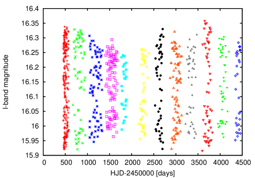
In the case of WVir stars things are more complicated. They should show increasing and decreasing period changes, since these stars are thought to undergo blue loops as they evolve from the AGB. From the stars included in the LITE analysis 12 WVir and 4 pWVir were in a possible binary system, and show period changes in both directions (with the exception of LMC-T2CEP-087, LMC-T2CEP-040, and SMC-T2CEP-001, where the period change was fixed to 0); see Tab. 2. Even more interestingly in Table 3 4 pWVir and 22 WVir stars show a significant period change. A known feature of WVir stars is the amplitude variations in their LCs (Soszyński et al. (2008, 2010b), or in detail e.g. Templeton & Henden (2007), or more recently Plachy et al. (2017)), while some of these changes can be interpreted as period doubling (see Moskalik & Buchler (1990, 1993); Smolec & Moskalik (2014); Smolec (2016)). In the case of a few of these stars there is a new feature in the behaviour of the LCs. One of the most prominent examples is OGLE-LMC-T2CEP-127, which is shown in Figure 11. While the different sections (shown with a different colour codes) in the LC have different amplitudes through the whole OGLE-III data set, they can all be phased with a single period of $P=12.6692$ days. When phased, it becomes apparent that the LC is changing its shape, not only the amplitude. This feature is something new and we will be looking into this in more detail in the future.

Figure 11: Segmented light curve of OGLE-LMC-T2CEP-127, showing the changes in the amplitude in the upper panel, and the phased light curve of OGLE-LMC-T2CEP-127, using a period of $P=12.6692$ days, in lower panel.

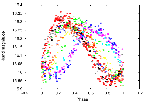
Stars showing this kind of behaviour are detected by LITE and can be found in either Table 2 or Table 3: OGLE-LMC-T2CEP-026, 034, 044, 072, 100, 127, and OGLE-SMC-T2CEP-14, 32, 34.

In the case of RVTs the increasingly erratic behaviour seen in their LCs, with alternating minima and maxima, and long-term amplitude changes on top of that, leads to detection of period change. The nature of the features seen in the infrared excess was discussed in Section 5.3. While these stars are thought to be crossing from cool to hot temperatures and should be showing period decrease, this is not what we see in the LITE results. Almost half of the RVT show a period increase. The interpretation of this phenomena is beyond the scope of this paper.

6 Summary and conclusions

The SEDs of 335 Type II and anomalous Cepheids in the Small and Large Magellanic Clouds have been constructed using photometry from the literature and fitted with a dust radiative transfer code. Luminosities and effective temperatures are derived from the fitting.

In a companion paper we use the derived luminosities and temperatures to discuss the period-luminosity and period-radius relation for T2Cs and ACs and to estimate the mass of these objects.

For $\sim 60\%$ of the RVT and $\sim 10\%$ of the (p)WVir objects, an infrared excess is detected from the SED fitting. For the RVT this is not unexpected as they are thought to evolve from the AGB to the PAGB phase. The results of Kamath et al. (2016) are confirmed that stars exist with luminosities below that predicted from single-star stellar evolution with IR excess, and the shape of the IR excess points to the presence of a disc rather than an expanding shell structure, which in turn suggests a relation to binarity.

Based on the shape of the phased LCs about one-third of the sample was selected to look for the light-time effect signature of a binary system following the method of Hajdu et al. (2015). Twenty-three systems appear to show the LITE, including a few known EBs. On the other hand LITE was not detected with any significance in seven known EBs.

The analysis of the (O-C) diagram also allows us to detect period changes and values for $\dot{P}$ are given for about 40 stars. Some of the period changes are much larger than predicted by standard evolution of single stars. Some are possibly related to the so-called binary evolutionary pulsators (BEP), the prototype of which, OGLE-BLG-RRLYR-02792, has a period change of $-8.4$ d/Myr ($-0.73$ s/yr) (Pietrzyński et al., 2012). Recently, Karczmarek et al. (2017) did extensive simulations to find contaminations of genuine RRL and classical Cepheids of 0.8 and 5%, respectively, by BEP. They did not specify numbers for T2Cs, but using their data we find a median crossing time of the IS of 36 kyr for stellar systems with luminosities between $\log L=2.4-2.9$ , which is similar to the 28 kyr they quote for RRL imposters. However the crossing time of a single star T2C is typically 10 times less than the 10 Myr they quote for RRL, so that a contamination of several percent is plausible.

The position of the objects in the HRD is compared to evolutionary tracks. In agreement with previous suggestions and predictions, the BLH can be explained by the evolution of $\sim$0.5-0.6 $M_{\odot}$ stars (depending on metallicity) evolving off the ZAHB and the ACs can be explained by the evolution of $\sim$1.1-2.3 $M_{\odot}$ stars. The evolution of the WVir subclass is not clear. They are at higher luminosities than the ACs and indeed evolutionary tracks of $\sim$2.5-4 $M_{\odot}$ stars cross this region in the HRD, but the periods of the WVir are longer than those of the short period classical Cepheids at these luminosities, which points to a lower mass. Also the evolutionary timescale does not fit this picture. It is shown that when a low-mass AGB star experiences a thermal pulse when the envelope mass is small, it can make a blue loop into the IS region of the WVir stars. But the timescale is extremely short, so this is also no explanation for the WVir as a class. The connection to binarity might be at the origin of the WVir stars, which has already been explicitly suggested for the peculiar W Virginis stars.

Appendix A Results of the fitting of the SEDs

Table 3 lists in Cols. 1-3 the OGLE name, type, and subtype of the object. Column 4 gives the pulsation period in days as reported by OGLE. The remaining columns refer to the results of fitting the SEDs: luminosity with error, effective temperature with error, dust optical depth, dust temperature at the inner radius, and whether this parameter was fixed (fit=0) or fitted (fit=1). The remarks column contains additional information, i.e. either regarding the pulsation period from Alcock et al. (1998, 2002) or the possibility of (weak) IR excess emission not considered in the fitting.

Table 3: Fit parameters

Name	Type	Subtype	Period	Luminosity	$T_{\rm eff}$	$\tau$	$T_{\rm c}$	fit	Remarks
			(d)	($L_{\odot}$)	(K)		(K)
OGLE-LMC-ACEP-001	ANCEP	F	0.850	78 $\pm$ 3	6125 $\pm$ 188	0.000	1000	0
OGLE-LMC-ACEP-002	ANCEP	F	0.977	119 $\pm$ 5	6250 $\pm$ 188	0.000	1000	0
OGLE-LMC-ACEP-003	ANCEP	1O	0.382	66 $\pm$ 2	6750 $\pm$ 250	0.000	1000	0
OGLE-LMC-ACEP-004	ANCEP	F	1.862	200 $\pm$ 17	6000 $\pm$ 812	0.000	1000	0
OGLE-LMC-ACEP-005	ANCEP	F	0.932	92 $\pm$ 1	6125 $\pm$ 188	0.000	1000	0
OGLE-LMC-ACEP-006	ANCEP	1O	0.850	200 $\pm$ 5	6250 $\pm$ 188	0.000	1000	0
OGLE-LMC-ACEP-007	ANCEP	F	0.896	114 $\pm$ 4	6375 $\pm$ 250	0.000	1000	0
OGLE-LMC-ACEP-008	ANCEP	1O	0.749	168 $\pm$ 5	6375 $\pm$ 125	0.000	1000	0
OGLE-LMC-ACEP-009	ANCEP	1O	0.800	153 $\pm$ 3	6250 $\pm$ 125	0.000	1000	0
OGLE-LMC-ACEP-010	ANCEP	F	0.834	81 $\pm$ 3	6250 $\pm$ 312	0.000	1000	0
OGLE-LMC-ACEP-011	ANCEP	F	0.999	118 $\pm$ 7	5625 $\pm$ 250	0.000	1000	0
OGLE-LMC-ACEP-012	ANCEP	F	0.829	107 $\pm$ 12	5875 $\pm$ 1062	0.000	1000	0
OGLE-LMC-ACEP-013	ANCEP	1O	0.501	77 $\pm$ 3	6250 $\pm$ 500	0.000	1000	0
OGLE-LMC-ACEP-014	ANCEP	F	2.291	299 $\pm$ 7	6125 $\pm$ 125	0.000	1000	0
OGLE-LMC-ACEP-015	ANCEP	1O	1.181	218 $\pm$ 4	6375 $\pm$ 188	0.000	1000	0
OGLE-LMC-ACEP-016	ANCEP	F	1.546	214 $\pm$ 9	6250 $\pm$ 188	0.000	1000	0
OGLE-LMC-ACEP-017	ANCEP	F	0.930	127 $\pm$ 3	6250 $\pm$ 125	0.000	1000	0
OGLE-LMC-ACEP-018	ANCEP	F	1.019	124 $\pm$ 4	6500 $\pm$ 312	0.000	1000	0
OGLE-LMC-ACEP-019	ANCEP	F	0.909	159 $\pm$ 3	6750 $\pm$ 188	0.000	1000	0
OGLE-LMC-ACEP-020	ANCEP	1O	0.382	100 $\pm$ 4	7375 $\pm$ 312	0.000	1000	0
OGLE-LMC-ACEP-021	ANCEP	F	1.296	159 $\pm$ 7	6125 $\pm$ 562	0.000	1000	0
OGLE-LMC-ACEP-023	ANCEP	1O	0.723	190 $\pm$ 9	6375 $\pm$ 188	0.000	1000	0
OGLE-LMC-ACEP-024	ANCEP	F	0.794	139 $\pm$ 3	7500 $\pm$ 125	0.000	1000	0
OGLE-LMC-ACEP-025	ANCEP	1O	0.474	100 $\pm$ 6	7000 $\pm$ 500	0.000	1000	0
OGLE-LMC-ACEP-026	ANCEP	F	1.739	228 $\pm$ 3	5875 $\pm$ 125	0.000	1000	0
OGLE-LMC-ACEP-027	ANCEP	F	1.267	222 $\pm$ 10	6500 $\pm$ 312	0.000	1000	0
OGLE-LMC-ACEP-028	ANCEP	1O	0.599	111 $\pm$ 5	5375 $\pm$ 312	0.000	1000	0
OGLE-LMC-ACEP-029	ANCEP	F	0.802	77 $\pm$ 2	6625 $\pm$ 250	0.000	1000	0
OGLE-LMC-ACEP-030	ANCEP	1O	0.667	173 $\pm$ 6	6500 $\pm$ 250	0.000	1000	0
OGLE-LMC-ACEP-031	ANCEP	1O	0.840	167 $\pm$ 7	6375 $\pm$ 438	0.000	1000	0
OGLE-LMC-ACEP-032	ANCEP	F	1.316	174 $\pm$ 4	6000 $\pm$ 125	0.000	1000	0
OGLE-LMC-ACEP-033	ANCEP	F	2.347	294 $\pm$ 5	6000 $\pm$ 125	0.000	1000	0
OGLE-LMC-ACEP-034	ANCEP	F	0.734	96 $\pm$ 8	6375 $\pm$ 812	0.000	1000	0
OGLE-LMC-ACEP-035	ANCEP	1O	0.446	76 $\pm$ 1	6625 $\pm$ 125	0.000	1000	0
OGLE-LMC-ACEP-036	ANCEP	F	1.258	170 $\pm$ 3	6000 $\pm$ 125	0.000	1000	0
OGLE-LMC-ACEP-037	ANCEP	F	1.258	258 $\pm$ 17	5125 $\pm$ 375	0.000	1000	0
OGLE-LMC-ACEP-038	ANCEP	F	1.335	164 $\pm$ 4	6375 $\pm$ 188	0.000	1000	0
OGLE-LMC-ACEP-039	ANCEP	F	0.992	115 $\pm$ 1	6375 $\pm$ 62	0.000	1000	0
OGLE-LMC-ACEP-040	ANCEP	F	0.961	136 $\pm$ 5	6000 $\pm$ 375	0.000	1000	0
OGLE-LMC-ACEP-041	ANCEP	F	0.878	101 $\pm$ 7	6250 $\pm$ 688	0.000	1000	0
OGLE-LMC-ACEP-042	ANCEP	F	1.079	82 $\pm$ 3	5000 $\pm$ 125	0.000	1000	0
OGLE-LMC-ACEP-043	ANCEP	1O	0.506	85 $\pm$ 1	6000 $\pm$ 125	0.000	1000	0
OGLE-LMC-ACEP-044	ANCEP	F	1.309	229 $\pm$ 11	6750 $\pm$ 312	0.000	1000	0
OGLE-LMC-ACEP-045	ANCEP	F	0.678	59 $\pm$ 1	6125 $\pm$ 250	0.000	1000	0
OGLE-LMC-ACEP-046	ANCEP	F	1.264	179 $\pm$ 11	6375 $\pm$ 500	0.000	1000	0
OGLE-LMC-ACEP-047	ANCEP	F	2.178	237 $\pm$ 8	6375 $\pm$ 188	0.000	1000	0
OGLE-LMC-ACEP-048	ANCEP	F	1.546	230 $\pm$ 12	6000 $\pm$ 438	0.000	1000	0
OGLE-LMC-ACEP-049	ANCEP	F	0.645	89 $\pm$ 6	6875 $\pm$ 562	0.000	1000	0
OGLE-LMC-ACEP-050	ANCEP	1O	1.045	335 $\pm$ 9	6750 $\pm$ 125	0.000	1000	0
OGLE-LMC-ACEP-051	ANCEP	F	0.709	68 $\pm$ 1	6125 $\pm$ 62	0.000	1000	0
OGLE-LMC-ACEP-052	ANCEP	F	1.263	191 $\pm$ 9	6125 $\pm$ 312	0.000	1000	0
OGLE-LMC-ACEP-053	ANCEP	F	1.888	267 $\pm$ 12	5750 $\pm$ 375	0.000	1000	0
OGLE-LMC-ACEP-054	ANCEP	F	0.980	82 $\pm$ 2	5375 $\pm$ 188	0.000	1000	0
OGLE-LMC-ACEP-055	ANCEP	F	1.607	188 $\pm$ 10	5875 $\pm$ 375	0.000	1000	0
OGLE-LMC-ACEP-056	ANCEP	F	1.124	144 $\pm$ 7	6125 $\pm$ 500	0.000	1000	0
OGLE-LMC-ACEP-057	ANCEP	F	1.710	250 $\pm$ 6	6000 $\pm$ 188	0.000	1000	0
OGLE-LMC-ACEP-058	ANCEP	1O	0.485	142 $\pm$ 9	7875 $\pm$ 812	0.000	1000	0
OGLE-LMC-ACEP-059	ANCEP	F	0.835	42 $\pm$ 2	4500 $\pm$ 188	0.000	1000	0
OGLE-LMC-ACEP-060	ANCEP	F	1.276	221 $\pm$ 4	6375 $\pm$ 250	0.000	1000	0

Table 1: Continued

Name	Type	Subtype	Period	Luminosity	$T_{\rm eff}$	$\tau$	$T_{\rm c}$	fit	Remarks
			(d)	($L_{\odot}$)	(K)		(K)
OGLE-LMC-ACEP-061	ANCEP	F	0.848	99 $\pm$ 2	6125 $\pm$ 188	0.000	1000	0
OGLE-LMC-ACEP-062	ANCEP	F	1.059	216 $\pm$ 14	7000 $\pm$ 500	0.000	1000	0
OGLE-LMC-ACEP-063	ANCEP	F	0.893	70 $\pm$ 2	5625 $\pm$ 250	0.000	1000	0
OGLE-LMC-ACEP-064	ANCEP	F	1.357	203 $\pm$ 4	6250 $\pm$ 250	0.000	1000	0
OGLE-LMC-ACEP-065	ANCEP	F	1.322	195 $\pm$ 10	6500 $\pm$ 438	0.000	1000	0
OGLE-LMC-ACEP-066	ANCEP	F	1.040	124 $\pm$ 3	6250 $\pm$ 250	0.000	1000	0
OGLE-LMC-ACEP-067	ANCEP	F	0.821	101 $\pm$ 11	5750 $\pm$ 1125	0.000	1000	0
OGLE-LMC-ACEP-068	ANCEP	F	0.626	65 $\pm$ 5	6875 $\pm$ 562	0.000	1000	0	IR excess?
OGLE-LMC-ACEP-069	ANCEP	F	1.538	254 $\pm$ 7	5875 $\pm$ 250	0.000	1000	0
OGLE-LMC-ACEP-070	ANCEP	1O	0.629	98 $\pm$ 3	6500 $\pm$ 312	0.000	1000	0
OGLE-LMC-ACEP-071	ANCEP	1O	0.676	171 $\pm$ 10	7125 $\pm$ 375	0.000	1000	0
OGLE-LMC-ACEP-072	ANCEP	F	1.048	201 $\pm$ 8	6500 $\pm$ 375	0.000	1000	0
OGLE-LMC-ACEP-073	ANCEP	F	1.465	255 $\pm$ 11	6375 $\pm$ 438	0.000	1000	0
OGLE-LMC-ACEP-074	ANCEP	F	1.533	221 $\pm$ 4	6250 $\pm$ 188	0.000	1000	0
OGLE-LMC-ACEP-075	ANCEP	F	0.692	88 $\pm$ 3	6500 $\pm$ 312	0.000	1000	0
OGLE-LMC-ACEP-076	ANCEP	F	1.582	193 $\pm$ 5	6250 $\pm$ 312	0.000	1000	0
OGLE-LMC-ACEP-077	ANCEP	F	1.122	129 $\pm$ 5	5875 $\pm$ 125	0.000	1000	0
OGLE-LMC-ACEP-078	ANCEP	1O	0.857	236 $\pm$ 5	6875 $\pm$ 188	0.000	1000	0
OGLE-LMC-ACEP-079	ANCEP	F	1.155	202 $\pm$ 10	6625 $\pm$ 250	0.000	1000	0
OGLE-LMC-ACEP-080	ANCEP	F	1.057	143 $\pm$ 3	6375 $\pm$ 250	0.000	1000	0
OGLE-LMC-ACEP-081	ANCEP	F	0.801	89 $\pm$ 3	6375 $\pm$ 188	0.000	1000	0
OGLE-LMC-ACEP-082	ANCEP	1O	0.775	154 $\pm$ 3	5625 $\pm$ 125	0.000	1000	0
OGLE-LMC-T2CEP-001	T2CEP	BLHer	1.814	101 $\pm$ 1	6000 $\pm$ 62	0.000	1000	0
OGLE-LMC-T2CEP-002	T2CEP	WVir	18.324	629 $\pm$ 29	5250 $\pm$ 312	0.000	1000	0
OGLE-LMC-T2CEP-003	T2CEP	RVTau	35.660	4228 $\pm$ 191	6000 $\pm$ 438	1.382	1300	0
OGLE-LMC-T2CEP-004	T2CEP	BLHer	1.916	143 $\pm$ 12	5625 $\pm$ 438	0.000	1000	0
OGLE-LMC-T2CEP-005	T2CEP	RVTau	33.185	1277 $\pm$ 136	4875 $\pm$ 312	0.000	1000	0
OGLE-LMC-T2CEP-006	T2CEP	BLHer	1.088	84 $\pm$ 3	7000 $\pm$ 312	0.000	1000	0
OGLE-LMC-T2CEP-007	T2CEP	BLHer	1.243	87 $\pm$ 3	6750 $\pm$ 250	0.000	1000	0
OGLE-LMC-T2CEP-008	T2CEP	BLHer	1.746	90 $\pm$ 2	5875 $\pm$ 125	0.000	1000	0
OGLE-LMC-T2CEP-009	T2CEP	BLHer	1.761	104 $\pm$ 2	6250 $\pm$ 125	0.000	1000	0
OGLE-LMC-T2CEP-010	T2CEP	BLHer	1.503	87 $\pm$ 2	6500 $\pm$ 250	0.000	1000	0
OGLE-LMC-T2CEP-011	T2CEP	RVTau	39.257	2893 $\pm$ 61	5875 $\pm$ 125	0.045	906	1
OGLE-LMC-T2CEP-012	T2CEP	WVir	11.581	419 $\pm$ 13	5250 $\pm$ 250	0.000	1000	0
OGLE-LMC-T2CEP-013	T2CEP	WVir	11.545	388 $\pm$ 8	5250 $\pm$ 125	0.000	1000	0
OGLE-LMC-T2CEP-014	T2CEP	RVTau	61.876	2325 $\pm$ 52	5750 $\pm$ 125	0.078	1100	0
OGLE-LMC-T2CEP-015	T2CEP	RVTau	56.521	2910 $\pm$ 53	5000 $\pm$ 125	0.261	1200	0	P=56.224 (Alcock et al., 1998)
OGLE-LMC-T2CEP-016	T2CEP	RVTau	20.296	1025 $\pm$ 54	6750 $\pm$ 312	0.122	600	0
OGLE-LMC-T2CEP-017	T2CEP	WVir	14.455	476 $\pm$ 19	4875 $\pm$ 188	0.000	1000	0
OGLE-LMC-T2CEP-018	T2CEP	BLHer	1.380	88 $\pm$ 1	6375 $\pm$ 125	0.000	1000	0
OGLE-LMC-T2CEP-019	T2CEP	pWVir	8.675	436 $\pm$ 35	5000 $\pm$ 750	0.000	1000	0
OGLE-LMC-T2CEP-020	T2CEP	BLHer	1.108	93 $\pm$ 4	6500 $\pm$ 312	0.000	1000	0
OGLE-LMC-T2CEP-021	T2CEP	pWVir	9.760	552 $\pm$ 14	5750 $\pm$ 125	0.000	1000	0	EB
OGLE-LMC-T2CEP-022	T2CEP	WVir	10.717	383 $\pm$ 8	5250 $\pm$ 188	0.000	1000	0	W3 excess
OGLE-LMC-T2CEP-023	T2CEP	pWVir	5.235	837 $\pm$ 26	6250 $\pm$ 250	0.000	1000	0	EB
OGLE-LMC-T2CEP-024	T2CEP	BLHer	1.247	75 $\pm$ 3	6500 $\pm$ 375	0.000	1000	0
OGLE-LMC-T2CEP-025	T2CEP	RVTau	67.965	2911 $\pm$ 179	4875 $\pm$ 312	0.000	1000	0	IR excess?
OGLE-LMC-T2CEP-026	T2CEP	WVir	13.578	443 $\pm$ 10	5000 $\pm$ 125	0.000	1000	0
OGLE-LMC-T2CEP-027	T2CEP	WVir	17.134	619 $\pm$ 25	5500 $\pm$ 375	0.000	1000	0	P=17.127 (Alcock et al., 1998)
OGLE-LMC-T2CEP-028	T2CEP	pWVir	8.785	833 $\pm$ 36	6375 $\pm$ 375	0.000	1000	0
OGLE-LMC-T2CEP-029	T2CEP	RVTau	31.245	2851 $\pm$ 79	5750 $\pm$ 188	1.347	746	1	P=31.716 (Alcock et al., 1998)
OGLE-LMC-T2CEP-030	T2CEP	BLHer	3.935	202 $\pm$ 5	5750 $\pm$ 125	0.000	1000	0
OGLE-LMC-T2CEP-031	T2CEP	WVir	6.706	253 $\pm$ 4	5375 $\pm$ 125	0.000	1000	0
OGLE-LMC-T2CEP-032	T2CEP	RVTau	44.561	3821 $\pm$ 590	4625 $\pm$ 1000	1.763	800	0
OGLE-LMC-T2CEP-033	T2CEP	pWVir	9.395	605 $\pm$ 14	5875 $\pm$ 250	0.000	1000	0	P=9.387 (Alcock et al., 1998)
OGLE-LMC-T2CEP-034	T2CEP	WVir	14.911	411 $\pm$ 14	4750 $\pm$ 125	0.000	1000	0	P=14.906 (Alcock et al., 1998)
OGLE-LMC-T2CEP-035	T2CEP	WVir	9.866	384 $\pm$ 16	5000 $\pm$ 250	0.000	1000	0

Table 1: Continued

Name	Type	Subtype	Period	Luminosity	$T_{\rm eff}$	$\tau$	$T_{\rm c}$	fit	Remarks
			(d)	($L_{\odot}$)	(K)		(K)
OGLE-LMC-T2CEP-036	T2CEP	WVir	14.881	501 $\pm$ 17	5625 $\pm$ 188	0.000	1000	0
OGLE-LMC-T2CEP-037	T2CEP	WVir	6.897	266 $\pm$ 4	5625 $\pm$ 125	0.000	1000	0
OGLE-LMC-T2CEP-038	T2CEP	WVir	4.014	537 $\pm$ 28	7250 $\pm$ 375	0.000	1000	0
OGLE-LMC-T2CEP-039	T2CEP	WVir	8.716	367 $\pm$ 13	5625 $\pm$ 250	0.000	1000	0	W3 excess
OGLE-LMC-T2CEP-040	T2CEP	pWVir	9.626	639 $\pm$ 31	5000 $\pm$ 375	0.000	1000	0	P=9.622 (Alcock et al., 1998)
OGLE-LMC-T2CEP-041	T2CEP	BLHer	2.476	290 $\pm$ 16	7250 $\pm$ 562	0.000	1000	0
OGLE-LMC-T2CEP-042	T2CEP	pWVir	4.923	384 $\pm$ 23	6750 $\pm$ 562	0.000	1000	0
OGLE-LMC-T2CEP-043	T2CEP	WVir	6.559	211 $\pm$ 5	5375 $\pm$ 188	0.000	1000	0
OGLE-LMC-T2CEP-044	T2CEP	WVir	13.270	439 $\pm$ 9	5250 $\pm$ 188	0.000	1000	0	P=13.246 (Alcock et al., 1998)
OGLE-LMC-T2CEP-045	T2CEP	RVTau	63.386	3479 $\pm$ 130	5125 $\pm$ 125	0.000	1000	0	IR excess?
OGLE-LMC-T2CEP-046	T2CEP	WVir	14.744	879 $\pm$ 21	5250 $\pm$ 125	0.718	809	1	P=14.752 (Alcock et al., 1998)
OGLE-LMC-T2CEP-047	T2CEP	WVir	7.286	285 $\pm$ 7	5500 $\pm$ 250	0.000	1000	0
OGLE-LMC-T2CEP-048	T2CEP	BLHer	1.445	92 $\pm$ 8	6375 $\pm$ 812	0.000	1000	0
OGLE-LMC-T2CEP-049	T2CEP	BLHer	3.235	231 $\pm$ 19	6375 $\pm$ 812	0.000	1000	0
OGLE-LMC-T2CEP-050	T2CEP	RVTau	34.748	1427 $\pm$ 34	5875 $\pm$ 125	0.117	1200	0
OGLE-LMC-T2CEP-051	T2CEP	RVTau	40.606	1850 $\pm$ 49	5500 $\pm$ 188	0.000	1000	0
OGLE-LMC-T2CEP-052	T2CEP	pWVir	4.688	448 $\pm$ 29	7000 $\pm$ 500	0.000	1000	0	EB
OGLE-LMC-T2CEP-053	T2CEP	BLHer	1.043	81 $\pm$ 2	6625 $\pm$ 188	0.000	1000	0
OGLE-LMC-T2CEP-054	T2CEP	WVir	9.925	338 $\pm$ 4	5125 $\pm$ 62	0.000	1000	0
OGLE-LMC-T2CEP-055	T2CEP	RVTau	41.005	2545 $\pm$ 77	5750 $\pm$ 188	0.080	1000	0
OGLE-LMC-T2CEP-056	T2CEP	WVir	7.290	246 $\pm$ 3	5125 $\pm$ 62	0.000	1000	0
OGLE-LMC-T2CEP-057	T2CEP	WVir	16.632	569 $\pm$ 19	5125 $\pm$ 312	0.000	1000	0	P=16.602 (Alcock et al., 1998)
OGLE-LMC-T2CEP-058	T2CEP	RVTau	21.483	715 $\pm$ 24	5125 $\pm$ 312	0.000	1000	0	P=21.486 (Alcock et al., 1998)
OGLE-LMC-T2CEP-059	T2CEP	WVir	16.736	720 $\pm$ 26	5125 $\pm$ 250	0.000	1000	0	P=16.747 (Alcock et al., 1998)
OGLE-LMC-T2CEP-060	T2CEP	BLHer	1.237	73 $\pm$ 4	6250 $\pm$ 688	0.000	1000	0
OGLE-LMC-T2CEP-061	T2CEP	BLHer	1.182	82 $\pm$ 5	7125 $\pm$ 562	0.000	1000	0
OGLE-LMC-T2CEP-062	T2CEP	WVir	6.047	190 $\pm$ 19	4750 $\pm$ 438	0.000	1000	0
OGLE-LMC-T2CEP-063	T2CEP	WVir	6.925	278 $\pm$ 8	5625 $\pm$ 250	0.000	1000	0
OGLE-LMC-T2CEP-064	T2CEP	BLHer	2.128	121 $\pm$ 8	6125 $\pm$ 750	0.000	1000	0
OGLE-LMC-T2CEP-065	T2CEP	RVTau	35.055	1563 $\pm$ 20	5375 $\pm$ 125	0.100	120	0
OGLE-LMC-T2CEP-066	T2CEP	WVir	13.109	412 $\pm$ 6	5125 $\pm$ 62	0.000	500	0
OGLE-LMC-T2CEP-067	T2CEP	RVTau	48.232	6429 $\pm$ 305	6125 $\pm$ 500	1.743	1200	0	P=48.539 (Alcock et al., 1998)
OGLE-LMC-T2CEP-068	T2CEP	BLHer	1.609	106 $\pm$ 2	6500 $\pm$ 250	0.000	1000	0
OGLE-LMC-T2CEP-069	T2CEP	BLHer	1.021	93 $\pm$ 14	6625 $\pm$ 1062	0.000	1000	0
OGLE-LMC-T2CEP-070	T2CEP	WVir	15.438	675 $\pm$ 36	5875 $\pm$ 312	0.000	1000	0	W3 excess
OGLE-LMC-T2CEP-071	T2CEP	BLHer	1.152	76 $\pm$ 9	6375 $\pm$ 875	0.000	1000	0
OGLE-LMC-T2CEP-072	T2CEP	WVir	14.514	534 $\pm$ 11	5375 $\pm$ 125	0.000	1000	0
OGLE-LMC-T2CEP-073	T2CEP	BLHer	3.088	169 $\pm$ 5	5875 $\pm$ 250	0.000	1000	0
OGLE-LMC-T2CEP-074	T2CEP	WVir	8.988	456 $\pm$ 9	5625 $\pm$ 188	0.000	1000	0
OGLE-LMC-T2CEP-075	T2CEP	RVTau	50.187	1868 $\pm$ 68	5125 $\pm$ 125	0.087	646	1
OGLE-LMC-T2CEP-076	T2CEP	BLHer	2.104	89 $\pm$ 3	5500 $\pm$ 312	0.000	1000	0
OGLE-LMC-T2CEP-077	T2CEP	BLHer	1.214	132 $\pm$ 5	7500 $\pm$ 375	0.000	1000	0	EB
OGLE-LMC-T2CEP-078	T2CEP	pWVir	6.716	404 $\pm$ 14	4875 $\pm$ 125	0.000	1000	0
OGLE-LMC-T2CEP-079	T2CEP	WVir	14.845	344 $\pm$ 19	4875 $\pm$ 188	0.000	1000	0	P=14.855 (Alcock et al., 1998)
OGLE-LMC-T2CEP-080	T2CEP	RVTau	40.916	2395 $\pm$ 104	5625 $\pm$ 250	0.113	331	1	P=41.118 (Alcock et al., 1998)
OGLE-LMC-T2CEP-081	T2CEP	WVir	9.480	369 $\pm$ 7	5375 $\pm$ 125	0.000	1000	0
OGLE-LMC-T2CEP-082	T2CEP	RVTau	35.124	1127 $\pm$ 75	5125 $\pm$ 312	0.000	1000	0
OGLE-LMC-T2CEP-083	T2CEP	pWVir	5.968	284 $\pm$ 6	5625 $\pm$ 125	0.000	1000	0
OGLE-LMC-T2CEP-084	T2CEP	BLHer	1.771	260 $\pm$ 40	7750 $\pm$ 1562	0.000	1000	0	EB
OGLE-LMC-T2CEP-085	T2CEP	BLHer	3.405	177 $\pm$ 6	6250 $\pm$ 375	0.000	1000	0
OGLE-LMC-T2CEP-086	T2CEP	WVir	15.845	665 $\pm$ 15	5500 $\pm$ 188	0.000	1000	0
OGLE-LMC-T2CEP-087	T2CEP	WVir	5.185	213 $\pm$ 9	5500 $\pm$ 438	0.000	1000	0
OGLE-LMC-T2CEP-088	T2CEP	BLHer	1.951	223 $\pm$ 11	8000 $\pm$ 375	0.000	1000	0
OGLE-LMC-T2CEP-089	T2CEP	BLHer	1.167	88 $\pm$ 2	6750 $\pm$ 188	0.000	1000	0
OGLE-LMC-T2CEP-090	T2CEP	BLHer	1.479	96 $\pm$ 2	6250 $\pm$ 250	0.000	1000	0

Table 1: Continued

Name	Type	Subtype	Period	Luminosity	$T_{\rm eff}$	$\tau$	$T_{\rm c}$	fit	Remarks
			(d)	($L_{\odot}$)	(K)		(K)
OGLE-LMC-T2CEP-091	T2CEP	RVTau	35.749	3880 $\pm$ 319	6625 $\pm$ 625	1.259	1100	0
OGLE-LMC-T2CEP-092	T2CEP	BLHer	2.617	133 $\pm$ 7	6000 $\pm$ 625	0.000	1000	0
OGLE-LMC-T2CEP-093	T2CEP	WVir	17.593	1211 $\pm$ 46	5875 $\pm$ 250	0.000	1000	0	EB, P=17.560 (Alcock et al., 1998)
									P=17.68586 (Alcock et al., 2002)
OGLE-LMC-T2CEP-094	T2CEP	WVir	8.468	285 $\pm$ 8	5000 $\pm$ 125	0.000	1000	0
OGLE-LMC-T2CEP-095	T2CEP	WVir	5.000	187 $\pm$ 3	5375 $\pm$ 62	0.000	1000	0
OGLE-LMC-T2CEP-096	T2CEP	WVir	13.926	498 $\pm$ 15	5375 $\pm$ 312	0.000	1000	0	P=13.925 (Alcock et al., 1998)
OGLE-LMC-T2CEP-097	T2CEP	WVir	10.510	423 $\pm$ 10	5500 $\pm$ 250	0.000	1000	0	P=10.509 (Alcock et al., 1998)
OGLE-LMC-T2CEP-098	T2CEP	pWVir	4.974	2857 $\pm$ 169	7375 $\pm$ 312	0.000	1000	0	EB, P=4.97371 (Alcock et al., 2002)
OGLE-LMC-T2CEP-099	T2CEP	WVir	15.487	516 $\pm$ 17	4625 $\pm$ 188	0.000	1000	0
OGLE-LMC-T2CEP-100	T2CEP	WVir	7.431	265 $\pm$ 5	5875 $\pm$ 188	0.000	1000	0
OGLE-LMC-T2CEP-101	T2CEP	WVir	11.419	499 $\pm$ 17	5875 $\pm$ 375	0.000	1000	0	P=11.442 (Alcock et al., 1998)
OGLE-LMC-T2CEP-102	T2CEP	BLHer	1.266	115 $\pm$ 5	6875 $\pm$ 438	0.000	1000	0
OGLE-LMC-T2CEP-103	T2CEP	WVir	12.908	454 $\pm$ 12	5375 $\pm$ 250	0.000	1000	0	P=12.902 (Alcock et al., 1998)
OGLE-LMC-T2CEP-104	T2CEP	RVTau	24.880	1889 $\pm$ 54	5500 $\pm$ 438	1.168	1100	0	P=24.848 (Alcock et al., 1998)
OGLE-LMC-T2CEP-105	T2CEP	BLHer	1.489	117 $\pm$ 6	6500 $\pm$ 625	0.000	1000	0
OGLE-LMC-T2CEP-106	T2CEP	WVir	6.707	272 $\pm$ 6	5500 $\pm$ 188	0.000	1000	0
OGLE-LMC-T2CEP-107	T2CEP	BLHer	1.209	105 $\pm$ 5	5875 $\pm$ 562	0.000	1000	0
OGLE-LMC-T2CEP-108	T2CEP	RVTau	30.011	1654 $\pm$ 37	5750 $\pm$ 125	0.000	1000	0
OGLE-LMC-T2CEP-109	T2CEP	BLHer	1.415	18 $\pm$ 1	4125 $\pm$ 112	0.000	1000	0
OGLE-LMC-T2CEP-110	T2CEP	WVir	7.078	242 $\pm$ 7	5250 $\pm$ 250	0.000	1000	0
OGLE-LMC-T2CEP-111	T2CEP	WVir	7.496	289 $\pm$ 5	5500 $\pm$ 125	0.000	1000	0
OGLE-LMC-T2CEP-112	T2CEP	RVTau	39.398	3186 $\pm$ 137	6000 $\pm$ 188	0.091	1200	0
OGLE-LMC-T2CEP-113	T2CEP	BLHer	3.085	267 $\pm$ 26	6625 $\pm$ 688	0.000	1000	0
OGLE-LMC-T2CEP-114	ANCEP	F	1.091	68 $\pm$ 1	5250 $\pm$ 188	0.000	1000	0	Soszyński et al. (2015a)
OGLE-LMC-T2CEP-115	T2CEP	RVTau	24.967	768 $\pm$ 29	5000 $\pm$ 188	0.000	1000	0	P=24.935 (Alcock et al., 1998)
OGLE-LMC-T2CEP-116	T2CEP	BLHer	1.967	79 $\pm$ 3	5500 $\pm$ 312	0.000	1000	0
OGLE-LMC-T2CEP-117	T2CEP	WVir	6.629	258 $\pm$ 6	5500 $\pm$ 125	0.000	1000	0
OGLE-LMC-T2CEP-118	T2CEP	WVir	12.699	428 $\pm$ 12	5125 $\pm$ 188	0.000	1000	0	P=12.704 (Alcock et al., 1998)
OGLE-LMC-T2CEP-119	T2CEP	RVTau	33.825	3325 $\pm$ 290	6250 $\pm$ 625	1.440	1200	0
OGLE-LMC-T2CEP-120	T2CEP	WVir	4.559	185 $\pm$ 4	5500 $\pm$ 188	0.000	1000	0
OGLE-LMC-T2CEP-121	T2CEP	BLHer	2.061	104 $\pm$ 5	5875 $\pm$ 562	0.000	1000	0
OGLE-LMC-T2CEP-122	T2CEP	BLHer	1.539	63 $\pm$ 2	5750 $\pm$ 312	0.000	1000	0
OGLE-LMC-T2CEP-123	T2CEP	BLHer	1.003	84 $\pm$ 8	5000 $\pm$ 438	0.000	1000	0
OGLE-LMC-T2CEP-124	T2CEP	BLHer	1.735	83 $\pm$ 4	6000 $\pm$ 438	0.000	1000	0
OGLE-LMC-T2CEP-125	T2CEP	RVTau	33.034	1208 $\pm$ 53	5125 $\pm$ 250	0.000	1000	0	IR excess?
OGLE-LMC-T2CEP-126	T2CEP	WVir	16.327	467 $\pm$ 26	4750 $\pm$ 125	0.981	313	1
OGLE-LMC-T2CEP-127	T2CEP	WVir	12.669	536 $\pm$ 62	5500 $\pm$ 500	0.305	363	1
OGLE-LMC-T2CEP-128	T2CEP	WVir	18.493	834 $\pm$ 38	5125 $\pm$ 250	0.000	1000	0
OGLE-LMC-T2CEP-129	T2CEP	RVTau	62.509	3132 $\pm$ 80	6000 $\pm$ 125	0.091	700	0
OGLE-LMC-T2CEP-130	T2CEP	BLHer	1.945	123 $\pm$ 8	6375 $\pm$ 688	0.000	1000	0
OGLE-LMC-T2CEP-131	T2CEP	BLHer	1.413	65 $\pm$ 1	6000 $\pm$ 125	0.000	1000	0
OGLE-LMC-T2CEP-132	T2CEP	pWVir	10.018	540 $\pm$ 17	5625 $\pm$ 312	0.000	1000	0
OGLE-LMC-T2CEP-133	T2CEP	WVir	6.282	269 $\pm$ 7	5750 $\pm$ 250	0.000	1000	0
OGLE-LMC-T2CEP-134	T2CEP	pWVir	4.076	406 $\pm$ 8	6125 $\pm$ 250	0.000	1000	0
OGLE-LMC-T2CEP-135	T2CEP	RVTau	26.522	1047 $\pm$ 24	5000 $\pm$ 188	0.000	1000	0	P=26.594 (Alcock et al., 1998)
OGLE-LMC-T2CEP-136	T2CEP	BLHer	1.323	163 $\pm$ 21	5625 $\pm$ 1188	0.000	1000	0
OGLE-LMC-T2CEP-137	T2CEP	WVir	6.362	265 $\pm$ 9	5625 $\pm$ 375	0.000	1000	0
OGLE-LMC-T2CEP-138	T2CEP	BLHer	1.394	79 $\pm$ 12	5375 $\pm$ 1312	0.000	1000	0
OGLE-LMC-T2CEP-139	T2CEP	WVir	14.780	484 $\pm$ 13	5000 $\pm$ 125	0.000	1000	0
OGLE-LMC-T2CEP-140	T2CEP	BLHer	1.841	103 $\pm$ 3	6000 $\pm$ 312	0.000	1000	0
OGLE-LMC-T2CEP-141	T2CEP	BLHer	1.823	73 $\pm$ 3	5875 $\pm$ 438	0.000	1000	0
OGLE-LMC-T2CEP-142	T2CEP	BLHer	1.761	108 $\pm$ 2	5500 $\pm$ 62	0.000	1000	0
OGLE-LMC-T2CEP-143	T2CEP	WVir	14.570	548 $\pm$ 18	5750 $\pm$ 312	0.000	1000	0
OGLE-LMC-T2CEP-144	T2CEP	BLHer	1.937	103 $\pm$ 26	5375 $\pm$ 1312	0.000	1000	0
OGLE-LMC-T2CEP-145	T2CEP	BLHer	3.337	267 $\pm$ 21	6500 $\pm$ 688	0.000	1000	0
OGLE-LMC-T2CEP-146	T2CEP	WVir	10.080	298 $\pm$ 11	5000 $\pm$ 188	0.000	1000	0
OGLE-LMC-T2CEP-147	T2CEP	RVTau	46.796	7160 $\pm$ 259	6375 $\pm$ 312	1.528	621	1	P=46.542 (Alcock et al., 1998)
OGLE-LMC-T2CEP-148	T2CEP	BLHer	2.672	135 $\pm$ 4	6250 $\pm$ 250	0.000	1000	0
OGLE-LMC-T2CEP-149	T2CEP	RVTau	42.481	2741 $\pm$ 117	5750 $\pm$ 250	0.000	1000	0	P=42.079 (Alcock et al., 1998)
OGLE-LMC-T2CEP-150	T2CEP	WVir	5.493	496 $\pm$ 9	6500 $\pm$ 125	0.152	1100	0

Table 1: Continued

Name	Type	Subtype	Period	Luminosity	$T_{\rm eff}$	$\tau$	$T_{\rm c}$	fit	Remarks
			(d)	($L_{\odot}$)	(K)		(K)
OGLE-LMC-T2CEP-151	T2CEP	WVir	7.887	311 $\pm$ 7	5500 $\pm$ 250	0.000	1000	0
OGLE-LMC-T2CEP-152	T2CEP	WVir	9.315	356 $\pm$ 12	5250 $\pm$ 312	0.000	1000	0	P=9.309 (Alcock et al., 1998)
OGLE-LMC-T2CEP-153	T2CEP	BLHer	1.175	465 $\pm$ 19	8000 $\pm$ 250	0.000	1000	0
OGLE-LMC-T2CEP-154	T2CEP	pWVir	7.578	1071 $\pm$ 28	6750 $\pm$ 125	0.000	1000	0
OGLE-LMC-T2CEP-155	T2CEP	WVir	6.898	282 $\pm$ 13	5000 $\pm$ 438	0.000	1000	0
OGLE-LMC-T2CEP-156	T2CEP	WVir	15.387	581 $\pm$ 79	4875 $\pm$ 188	0.530	151	1	P=15.391 (Alcock et al., 1998)
OGLE-LMC-T2CEP-157	T2CEP	WVir	14.335	431 $\pm$ 10	5000 $\pm$ 125	0.000	1000	0	P=14.337 (Alcock et al., 1998)
OGLE-LMC-T2CEP-158	T2CEP	WVir	7.139	270 $\pm$ 9	5500 $\pm$ 188	0.150	300	0
OGLE-LMC-T2CEP-159	T2CEP	WVir	6.626	221 $\pm$ 3	5125 $\pm$ 62	0.000	1000	0
OGLE-LMC-T2CEP-160	T2CEP	BLHer	1.757	90 $\pm$ 3	5875 $\pm$ 375	0.000	1000	0
OGLE-LMC-T2CEP-161	T2CEP	WVir	8.532	548 $\pm$ 26	5125 $\pm$ 312	0.000	1000	0
OGLE-LMC-T2CEP-162	T2CEP	RVTau	30.394	1109 $\pm$ 44	5000 $\pm$ 188	0.183	1000	0	P=30.408 (Alcock et al., 1998)
OGLE-LMC-T2CEP-163	T2CEP	BLHer	1.694	140 $\pm$ 16	6250 $\pm$ 875	0.000	1000	0
OGLE-LMC-T2CEP-164	T2CEP	pWVir	8.495	550 $\pm$ 14	5500 $\pm$ 250	0.483	1300	0
OGLE-LMC-T2CEP-165	T2CEP	BLHer	1.241	35 $\pm$ 1	4875 $\pm$ 125	0.000	1000	0
OGLE-LMC-T2CEP-166	T2CEP	BLHer	2.111	211 $\pm$ 7	5625 $\pm$ 312	0.000	1000	0
OGLE-LMC-T2CEP-167	T2CEP	BLHer	2.312	99 $\pm$ 4	5375 $\pm$ 438	0.000	1000	0
OGLE-LMC-T2CEP-168	T2CEP	WVir	15.698	554 $\pm$ 15	5250 $\pm$ 125	0.000	1000	0
OGLE-LMC-T2CEP-169	T2CEP	RVTau	30.956	1893 $\pm$ 379	6250 $\pm$ 625	0.442	477	1	P=31.127 (Alcock et al., 1998)
OGLE-LMC-T2CEP-170	T2CEP	WVir	7.683	239 $\pm$ 3	5125 $\pm$ 62	0.000	1000	0
OGLE-LMC-T2CEP-171	T2CEP	BLHer	1.555	109 $\pm$ 6	6375 $\pm$ 562	0.000	1000	0
OGLE-LMC-T2CEP-172	T2CEP	WVir	11.221	334 $\pm$ 21	4875 $\pm$ 250	0.000	1000	0
OGLE-LMC-T2CEP-173	T2CEP	WVir	4.148	55 $\pm$ 3	3900 $\pm$ 112	0.000	1000	0
OGLE-LMC-T2CEP-174	T2CEP	RVTau	46.819	6549 $\pm$ 342	6000 $\pm$ 438	1.333	1100	0	P=47.019 (Alcock et al., 1998)
OGLE-LMC-T2CEP-175	T2CEP	WVir	9.326	331 $\pm$ 6	5250 $\pm$ 125	0.000	1000	0
OGLE-LMC-T2CEP-176	T2CEP	WVir	7.990	315 $\pm$ 4	5375 $\pm$ 125	0.000	1000	0
OGLE-LMC-T2CEP-177	T2CEP	WVir	15.036	440 $\pm$ 14	5000 $\pm$ 188	0.000	1000	0
OGLE-LMC-T2CEP-178	T2CEP	WVir	12.212	319 $\pm$ 11	5000 $\pm$ 188	0.000	1000	0
OGLE-LMC-T2CEP-179	T2CEP	WVir	8.050	230 $\pm$ 4	5000 $\pm$ 62	0.000	1000	0
OGLE-LMC-T2CEP-180	T2CEP	RVTau	30.996	3139 $\pm$ 182	5500 $\pm$ 500	1.467	700	0
OGLE-LMC-T2CEP-181	T2CEP	pWVir	7.213	427 $\pm$ 24	5375 $\pm$ 312	0.000	1000	0
OGLE-LMC-T2CEP-182	T2CEP	WVir	8.226	372 $\pm$ 9	5250 $\pm$ 125	0.000	1000	0	P=8.240 (Alcock et al., 1998)
OGLE-LMC-T2CEP-183	T2CEP	WVir	6.510	145 $\pm$ 8	4625 $\pm$ 125	0.000	1000	0
OGLE-LMC-T2CEP-184	T2CEP	WVir	14.840	309 $\pm$ 16	4625 $\pm$ 188	0.000	1000	0
OGLE-LMC-T2CEP-185	T2CEP	WVir	12.688	1842 $\pm$ 33	4625 $\pm$ 62	0.000	1000	0
OGLE-LMC-T2CEP-186	T2CEP	WVir	16.362	519 $\pm$ 16	4875 $\pm$ 125	0.000	1000	0
OGLE-LMC-T2CEP-187	T2CEP	BLHer	2.404	96 $\pm$ 4	5500 $\pm$ 375	0.000	1000	0
OGLE-LMC-T2CEP-188	T2CEP	BLHer	1.049	87 $\pm$ 4	6125 $\pm$ 375	0.000	1000	0
OGLE-LMC-T2CEP-189	T2CEP	BLHer	1.308	79 $\pm$ 2	6250 $\pm$ 125	0.000	1000	0
OGLE-LMC-T2CEP-190	T2CEP	RVTau	38.362	2450 $\pm$ 56	5625 $\pm$ 188	0.019	700	0
OGLE-LMC-T2CEP-191	T2CEP	RVTau	34.345	3969 $\pm$ 127	5750 $\pm$ 250	1.251	700	0
OGLE-LMC-T2CEP-192	T2CEP	RVTau	26.194	916 $\pm$ 32	5375 $\pm$ 250	0.000	1000	0
OGLE-LMC-T2CEP-193	T2CEP	WVir	7.005	273 $\pm$ 4	5250 $\pm$ 62	0.000	1000	0
OGLE-LMC-T2CEP-194	T2CEP	BLHer	1.314	101 $\pm$ 5	6375 $\pm$ 250	0.000	1000	0
OGLE-LMC-T2CEP-195	T2CEP	BLHer	2.753	141 $\pm$ 5	5875 $\pm$ 312	0.000	1000	0
OGLE-LMC-T2CEP-196	T2CEP	WVir	14.958	668 $\pm$ 20	5125 $\pm$ 188	0.000	1000	0
OGLE-LMC-T2CEP-197	T2CEP	BLHer	1.224	96 $\pm$ 7	6375 $\pm$ 438	0.000	1000	0
OGLE-LMC-T2CEP-198	T2CEP	RVTau	38.274	908 $\pm$ 32	4500 $\pm$ 125	0.000	1000	0
OGLE-LMC-T2CEP-199	T2CEP	RVTau	37.204	7090 $\pm$ 338	8600 $\pm$ 300	0.024	1000	0
OGLE-LMC-T2CEP-200	T2CEP	RVTau	34.917	1695 $\pm$ 114	4875 $\pm$ 375	1.158	700	0
OGLE-LMC-T2CEP-201	T2CEP	pWVir	11.007	2172 $\pm$ 84	6500 $\pm$ 250	0.150	180	0
OGLE-LMC-T2CEP-202	T2CEP	RVTau	38.136	1028 $\pm$ 24	4625 $\pm$ 125	0.000	1000	0
OGLE-LMC-T2CEP-203	T2CEP	RVTau	37.127	887 $\pm$ 36	4625 $\pm$ 188	0.000	1000	0

Table 1: Continued

Name	Type	Subtype	Period	Luminosity	$T_{\rm eff}$	$\tau$	$T_{\rm c}$	fit	Remarks
			(d)	($L_{\odot}$)	(K)		(K)
OGLE-SMC-ACEP-01	ANCEP	1O	0.621	118 $\pm$ 3	7250 $\pm$ 188	0.000	1000	0
OGLE-SMC-ACEP-02	ANCEP	F	0.828	78 $\pm$ 1	6125 $\pm$ 62	0.000	1000	0
OGLE-SMC-ACEP-03	ANCEP	1O	0.570	103 $\pm$ 3	7125 $\pm$ 250	0.000	1000	0
OGLE-SMC-ACEP-04	ANCEP	F	0.830	100 $\pm$ 1	6375 $\pm$ 125	0.000	1000	0
OGLE-SMC-ACEP-05	ANCEP	1O	0.521	99 $\pm$ 2	7000 $\pm$ 125	0.000	1000	0
OGLE-SMC-ACEP-06	ANCEP	F	1.256	167 $\pm$ 10	6875 $\pm$ 250	0.000	1000	0
OGLE-SMC-T2CEP-001	T2CEP	pWVir	11.869	2570 $\pm$ 102	6250 $\pm$ 125	0.000	1000	0
OGLE-SMC-T2CEP-002	T2CEP	BLHer	1.372	109 $\pm$ 4	6750 $\pm$ 312	0.000	1000	0
OGLE-SMC-T2CEP-003	T2CEP	WVir	4.360	173 $\pm$ 7	5875 $\pm$ 312	0.000	1000	0
OGLE-SMC-T2CEP-004	T2CEP	WVir	6.533	299 $\pm$ 14	5375 $\pm$ 375	0.000	1000	0
OGLE-SMC-T2CEP-005	T2CEP	WVir	8.206	282 $\pm$ 3	5375 $\pm$ 62	0.000	1000	0
OGLE-SMC-T2CEP-006	T2CEP	BLHer	1.236	80 $\pm$ 1	6375 $\pm$ 62	0.000	1000	0
OGLE-SMC-T2CEP-007	T2CEP	RVTau	30.961	7560 $\pm$ 1970	6125 $\pm$ 750	0.000	1000	0
OGLE-SMC-T2CEP-008	T2CEP	BLHer	1.490	117 $\pm$ 2	5875 $\pm$ 125	0.000	1000	0
OGLE-SMC-T2CEP-009	T2CEP	BLHer	2.971	151 $\pm$ 3	5625 $\pm$ 125	0.000	1000	0
OGLE-SMC-T2CEP-010	T2CEP	pWVir	17.481	4264 $\pm$ 319	6000 $\pm$ 312	0.000	1000	0
OGLE-SMC-T2CEP-011	T2CEP	pWVir	9.925	3758 $\pm$ 136	7250 $\pm$ 250	0.028	1000	0
OGLE-SMC-T2CEP-012	T2CEP	RVTau	29.219	1301 $\pm$ 41	5375 $\pm$ 62	0.000	1000	0
OGLE-SMC-T2CEP-013	T2CEP	WVir	13.810	478 $\pm$ 13	5375 $\pm$ 62	0.000	1000	0
OGLE-SMC-T2CEP-014	T2CEP	WVir	13.878	426 $\pm$ 8	5375 $\pm$ 62	0.000	1000	0
OGLE-SMC-T2CEP-015	T2CEP	BLHer	2.570	458 $\pm$ 21	7500 $\pm$ 312	0.000	1000	0
OGLE-SMC-T2CEP-016	T2CEP	BLHer	2.113	122 $\pm$ 3	6000 $\pm$ 188	0.000	1000	0
OGLE-SMC-T2CEP-017	T2CEP	BLHer	1.299	115 $\pm$ 5	6375 $\pm$ 375	0.000	1000	0
OGLE-SMC-T2CEP-018	T2CEP	RVTau	39.519	3539 $\pm$ 166	5875 $\pm$ 375	1.616	1200	0
OGLE-SMC-T2CEP-019	T2CEP	RVTau	40.912	3481 $\pm$ 101	6250 $\pm$ 125	0.037	598	1
OGLE-SMC-T2CEP-020	T2CEP	RVTau	50.623	1885 $\pm$ 84	5375 $\pm$ 188	0.000	1000	0
OGLE-SMC-T2CEP-021	T2CEP	BLHer	2.313	94 $\pm$ 1	6000 $\pm$ 125	0.000	1000	0
OGLE-SMC-T2CEP-022	T2CEP	BLHer	1.471	61 $\pm$ 2	6000 $\pm$ 250	0.000	1000	0
OGLE-SMC-T2CEP-023	T2CEP	pWVir	17.675	1508 $\pm$ 28	5750 $\pm$ 125	0.000	1000	0	EB
OGLE-SMC-T2CEP-024	T2CEP	RVTau	43.961	3075 $\pm$ 126	6000 $\pm$ 188	0.077	700	0
OGLE-SMC-T2CEP-025	T2CEP	pWVir	14.171	941 $\pm$ 34	5750 $\pm$ 125	0.000	1000	0
OGLE-SMC-T2CEP-026	T2CEP	BLHer	1.705	153 $\pm$ 2	6375 $\pm$ 125	0.000	1000	0
OGLE-SMC-T2CEP-027	T2CEP	BLHer	1.542	81 $\pm$ 2	6250 $\pm$ 125	0.000	1000	0
OGLE-SMC-T2CEP-028	T2CEP	pWVir	15.264	1854 $\pm$ 53	5375 $\pm$ 62	0.000	1000	0	EB
OGLE-SMC-T2CEP-029	T2CEP	RVTau	33.676	6273 $\pm$ 157	5375 $\pm$ 62	0.000	1000	0	EB
OGLE-SMC-T2CEP-030	T2CEP	BLHer	3.389	418 $\pm$ 9	6750 $\pm$ 188	0.000	1000	0
OGLE-SMC-T2CEP-031	T2CEP	WVir	7.895	323 $\pm$ 21	5375 $\pm$ 312	0.000	1000	0
OGLE-SMC-T2CEP-032	T2CEP	WVir	14.247	693 $\pm$ 30	5750 $\pm$ 188	0.086	600	0
OGLE-SMC-T2CEP-033	T2CEP	BLHer	1.878	198 $\pm$ 6	6375 $\pm$ 188	0.000	1000	0
OGLE-SMC-T2CEP-034	T2CEP	WVir	20.121	994 $\pm$ 39	5375 $\pm$ 62	0.000	1000	0
OGLE-SMC-T2CEP-035	T2CEP	WVir	17.181	730 $\pm$ 31	5500 $\pm$ 312	0.025	1100	0
OGLE-SMC-T2CEP-036	T2CEP	BLHer	1.092	141 $\pm$ 2	6500 $\pm$ 125	0.000	1000	0
OGLE-SMC-T2CEP-037	T2CEP	BLHer	1.559	127 $\pm$ 3	6125 $\pm$ 125	0.000	1000	0
OGLE-SMC-T2CEP-038	T2CEP	pWVir	4.444	734 $\pm$ 32	6500 $\pm$ 250	0.000	1000	0
OGLE-SMC-T2CEP-039	T2CEP	BLHer	1.888	142 $\pm$ 1	5875 $\pm$ 62	0.000	1000	0
OGLE-SMC-T2CEP-040	T2CEP	WVir	16.111	662 $\pm$ 64	5375 $\pm$ 312	0.000	1000	0
OGLE-SMC-T2CEP-041	T2CEP	RVTau	29.118	1393 $\pm$ 49	5750 $\pm$ 125	0.000	1000	0
OGLE-SMC-T2CEP-042	T2CEP	BLHer	1.487	100 $\pm$ 2	6250 $\pm$ 62	0.000	1000	0
OGLE-SMC-T2CEP-043	T2CEP	RVTau	23.743	1285 $\pm$ 57	5375 $\pm$ 125	0.000	1000	0	W3 excess

Appendix B The modelled SEDs

Figure 12 shows the fits to the photometry.

Figure 12: Fits to the SEDs.

Figure 1: Continued

Figure 1: Continued

Figure 1: Continued

Figure 1: Continued

Figure 1: Continued

Figure 1: Continued

Figure 1: Continued

Figure 1: Continued

Figure 1: Continued

Figure 1: Continued

Figure 1: Continued

Figure 1: Continued

Figure 1: Continued

Figure 1: Continued

Figure 1: Continued

Figure 1: Continued

Figure 1: Continued

Figure 1: Continued

Figure 1: Continued

Figure 1: Continued

Figure 1: Continued

Figure 1: Continued

Figure 1: Continued

Figure 1: Continued

Figure 1: Continued

Figure 1: Continued

Figure 1: Continued

Figure 1: Continued

Figure 1: Continued

Figure 1: Continued

Figure 1: Continued

Figure 1: Continued

Figure 1: Ccontinued

Appendix C The light-time travel effect

In this Appendix we describe the implementation of the method outlined in Hajdu et al. (2015) to construct O-C diagrams and investigate the presence of period changes or binarity based on the LITE. The code described below is written in Fortran77. The programme reads in an input file containing the name of the source, an estimate of a time of maximum light (typically near the midpoint of the available time series) and pulsation period, an estimate of the mean magnitude, the number of harmonics ($N$) to be fitted to the phased LC, and a file containing estimates of the Fourier coefficients of the LC. All these parameters are determined externally to the code, and specifically we use the publicly available code Period04 for this part (Lenz & Breger, 2005).

These parameters are read in the code, and in a first step, an $N$-term Fourier series (specifically in the form of Eq. 1 in Appendix A in Groenewegen (2004)) is fitted to the entire time series using the mrqmin routine from Numerical Recipes (Press et al., 1992). The LC and phased LC are inspected, and at this point some data may be removed from the time series, either photometric outliers, or, specifically in the case of EBs, data taken at the time of eclipses.

Then the code is run on a limited stretch of data to determine a well-defined template LC and its Fourier parameters are saved.

The next step is the determination of the O-C diagram. The DT consecutive data points in time are selected; DT is typically 50. The ”time” associated with this chunk of data is the median value of the individual observing times. Forty trial shifts in phase are examined over a total phase range ($\delta\phi$), which varies from star to star depending on the O-C variation relative to the period (see below). In the extreme case, 40 points increasing by 0.025 in phase would allow us to probe O-C variations from $-0.5P$ to $+0.5P$. For each trial shift, $j$, the template LC is compared to the actual LC and a reduced $\chi_{\rm r}^{2}$ determined. The key assumption in the entire method is that the template LC remains constant in time. This is a reasonable assumption for classical variables, but T2Cs often display amplitude modulations as well. To allow for this simplest of modification of a strictly time-independent template LC, a scaling of the Fourier amplitudes is applied in determining the $\chi_{\rm r}^{2}$. The index $j_{\rm min}$ of the lowest $\chi_{\rm r}^{2}$ is found and a parabola is fitted to the $\chi_{\rm r}^{2}$s at indices $j_{\rm min}-1$, $j_{\rm min}$, and $j_{\rm min}+1$ to determine the final best-fitting phase shift, hence O-C value, and final $\chi_{\rm r,min}^{2}$. This is repeated for the next DT number of points, etc. An error in O-C is determined by finding the roots of the parabolic equation at a value higher than $\chi_{\rm r,min}^{2}$. If $\chi^{2}_{\rm r,min}$ were of order unity this value would be $\chi^{2}_{\rm r,min}+1$ but this is rarely the case here. Practically, the errors are determined by finding the range in phase shifts at a level $(F\cdot\chi^{2}_{\rm r,min})$, where $F$ is typically 1.15 and ranges between 1.01 and 1.5 (see below). Also at this point the range in the values of $j_{\rm min}$ for the individual chuncks of data are known, and $\delta\phi$ can be changed so that these values cover roughly the range between 1 and 40.

The O-C diagram is plotted and a model can be fitted to the data. The model is a combination of a changing period ($\dot{P}$, $\ddot{P}$), and a binary model

$$(O-C)(t)=c_{0}+c_{1}t+c_{2}t^{2}+c_{3}t^{3}+...$$ (3)

$$\hskip 85.35826pt...+(a\sin i)\,\frac{1-e^{2}}{1+e\cos(\nu)}\,\sin(\nu+\omega),$$ (4)

where $a$ is the semi-major axis, $i$ is the inclination, $e$ is the eccentricity, and $\omega$ is the argument of the periastron. The true anomaly $\nu$ is a function of the time $t$, the orbital period $P_{\rm orb}$, the time of periastron passage $T_{\rm peri}$, and $e$. All parameters of the model ($c_{0},c_{1},c_{2},c_{3}$, $P_{\rm orb}$, $T_{\rm peri}$, $a\sin i$, $e$, $\omega$) can be fitted or fixed. Starting values for $c_{0},c_{1},c_{2},c_{3}$ are zero, if a binary model is used the initial values for $P_{\rm orb}$, $T_{\rm peri}$, $a\sin i$ are estimated from the O-C diagram. Some trial and error starting values are sometimes recommended, especially for non-zero eccentric orbits. The fitting is done again with the mrqmin routine. By changing the factor $F$ in the determination of the error in the individual O-C values the reduced $\chi^{2}$ of the model fit is tuned to be approximately unity. This then provides the model parameters and their errors.

The code was tested against the showcase example of BLG-RRL-06498 in Hajdu et al. (2015). The parameters are compared in Table 2 and the (phased) LC and O-C diagram and model fit are shown in Figure 2; cf. Fig. 2 in Hajdu et al. (2015). Initially only OGLE-III was available to us but in the course of this project the OGLE-IV data also became public via Soszyński et al. (2014), which were already available to Hajdu et al. (2015). Both solutions are given in the table illustrating the power of the increased time span of the observations. The derived parameters agree within the error.

Table 2 in the main text lists the systems where this investigation suggested a possible binary system based on the LITE (it includes known EBs). The (phased) LC and the O-C diagrams with the model fits are shown in Figure 4.

Table 3 lists the systems for which a significant period change is suggested; it includes known EBs for which the LITE could not be established. The (phased) LC and the O-C diagrams with the model fits are shown in Figure 4.

Table 4 lists the systems that were investigated but with inconclusive results regarding the LITE or significant period changes. Additional information is available from the first author.

Table 2: Comparison of results for BLG-RRL-06498

$P_{\rm bin}$	$T_{\rm peri}$	$e$	$\omega$	$a\sin i$	$\dot{P}$	Remarks
(d)	(JD-2450000)		(deg)	(AU)	(d/Myr)
2789 $\pm$ 18	8137 $\pm$ 134	0.12 $\pm$ 0.04	$-82\pm 16$	2.35 $\pm$ 0.05	$-0.11\leavevmode\nobreak\ \pm$ 0.03	Hajdu et al. (2015), based on OGLE-III + IV data
2804 $\pm$ 30	7917 $\pm$ 116	0.17 ${}^{+0.05}_{-0.04}$	$-85\pm 15$	2.45 $\pm$ 0.05	$+0.06\leavevmode\nobreak\ \pm$ 0.07	present paper, based on OGLE-III data
2766 $\pm$ 10	7931 $\pm$ 52	0.16 $\pm$ 0.02	$-73\pm 6$	2.42 $\pm$ 0.03	$-0.10\leavevmode\nobreak\ \pm$ 0.02	present paper, based on OGLE-III +IV data
3470 $\pm$ 160	7850 $\pm$ 64	0 (fixed)	–	276 $\pm$ 13	$+7000\leavevmode\nobreak\ \pm$ 350	OGLE-BLG-T2CEP-059
–	–	–	–	–	$+11200\leavevmode\nobreak\ \pm$ 200	OGLE-BLG-T2CEP-059, only period change

Figure 2: Light curves and O-C diagrams of BLG-RRL-06498. The left-hand panel shows the time series (top) and phased light curve (bottom). The right-hand panel shows the O-C diagram (top) and the residual after subtracting the model (bottom). The full model is represented by the full line. The contribution due to a changing period is indicated by the dotted line.

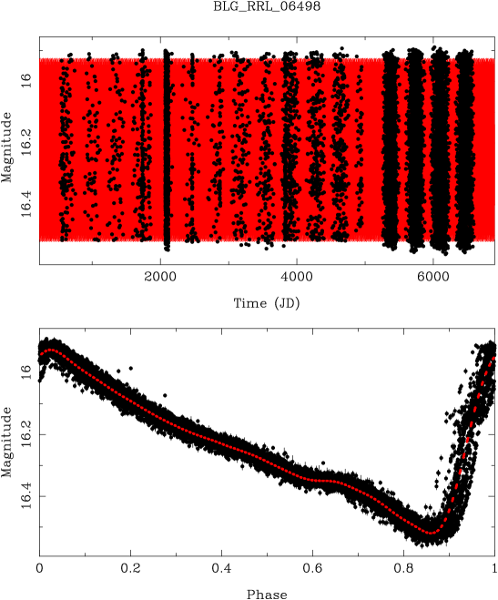
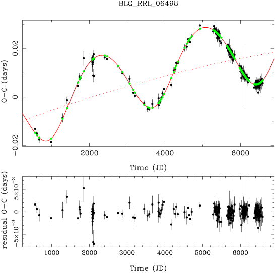
Figure 3 and Table 2 show the analysis of the system OGLE-BLG-T2CEP-059 that is mentioned in the main text and was noted by Soszyński et al. (2011) to have a large period change. The bottom left panel shows the result when only a period change is considered. A value of 11200 d/Myr is found but the plot with the residuals shows a pattern. Within the framework of the model that is used here a binary model would be proposed and the fits are shown in the bottom right panel. The residuals are flat within the errors. The period change is 7700 d/Myr in this model.

Figure 3: Light curves and O-C diagrams of BLG-T2CEP-059. The top left-hand and right-hand panels show the time series (top left), and phased light curve (top right) for a period of 12.637 days. The bottom panels show the O-C diagram for a model with only a period change (bottom left), and a binary + $\dot{P}$ model.

Figure 4: Light curves and O-C diagrams of candidate binary stars based on the LITE. The left-hand panel shows the time series (top) and phased light curve (bottom). The right-hand panel shows the O-C diagram (top) and the residual after subtracting the model (bottom). The full model is represented by the full line. The contribution due to a changing period is indicated by the dotted line.

Figure 3: Continued

Figure 3: Continued

Table 3: T2C with significant period change

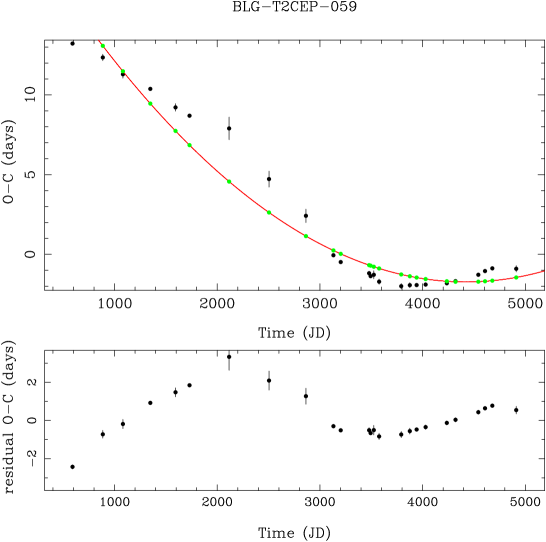
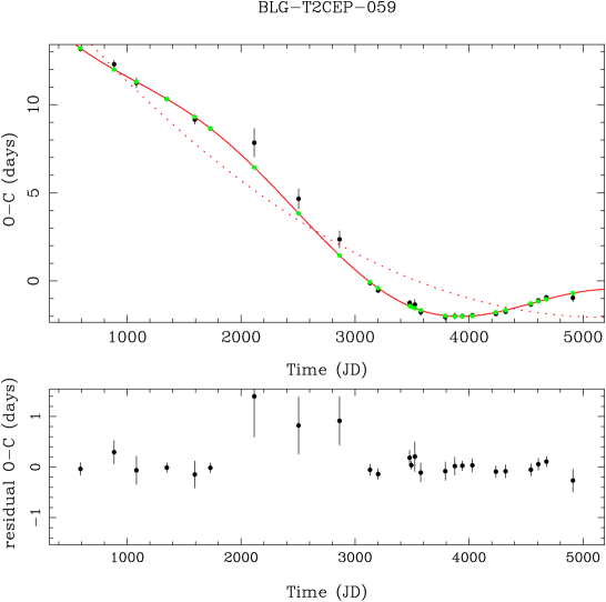
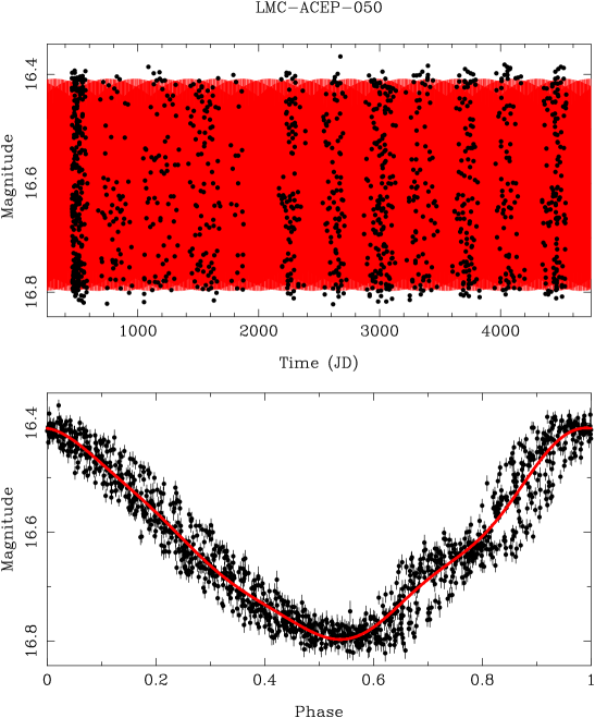
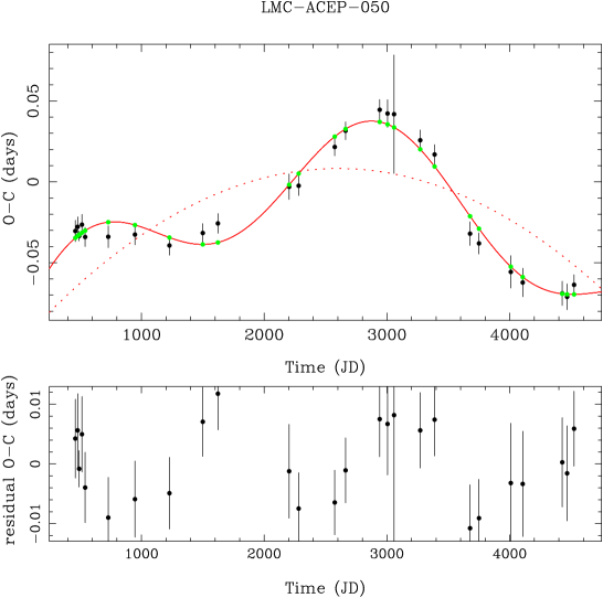
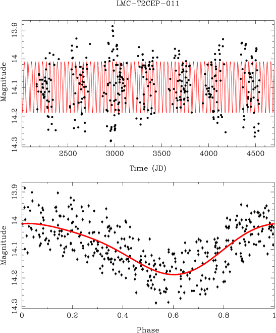
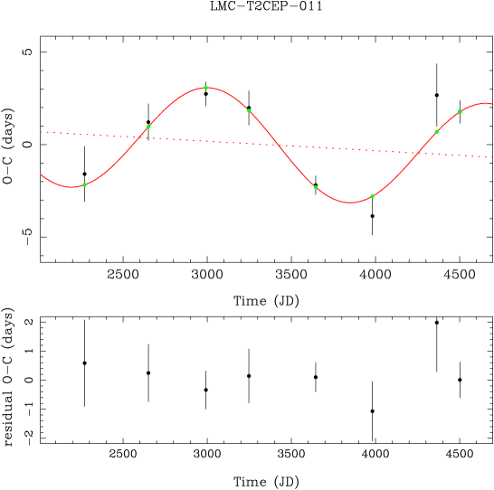
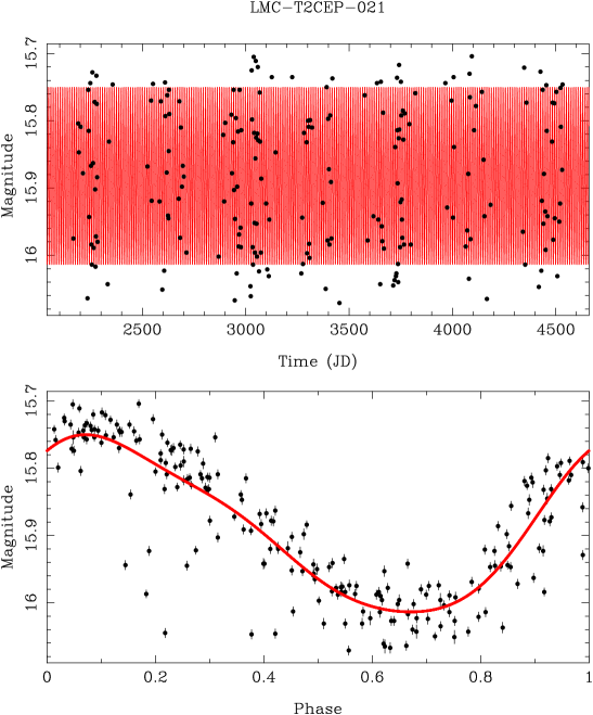
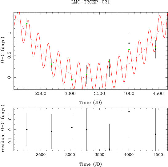
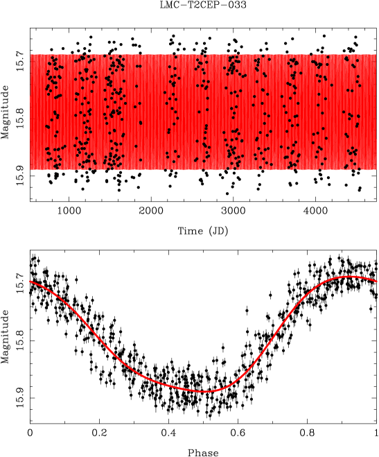
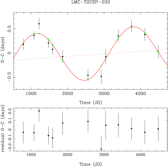
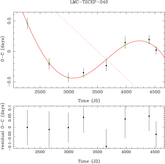
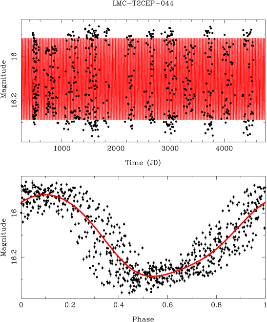
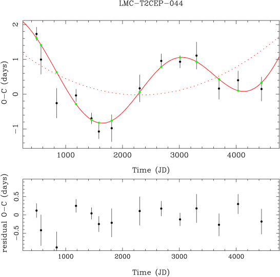
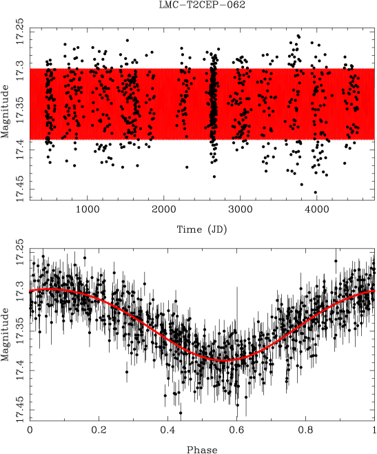
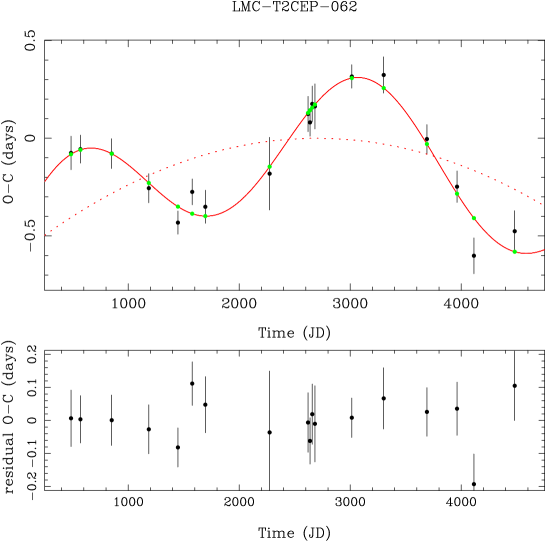
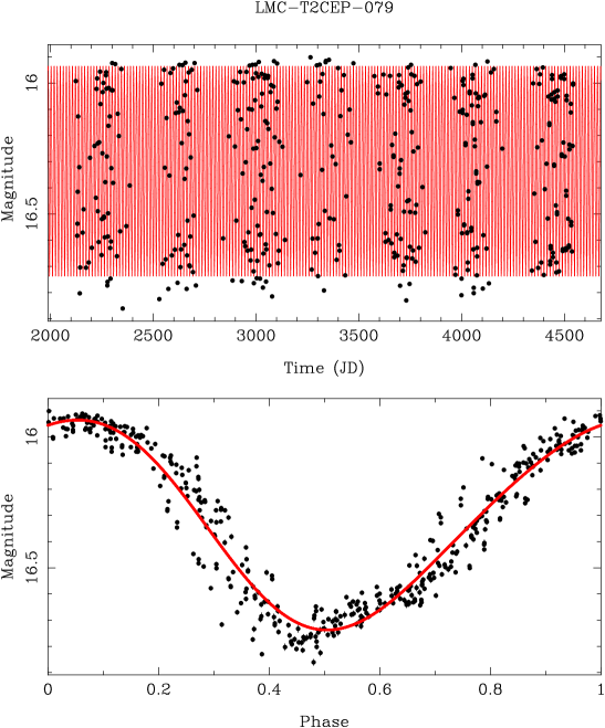
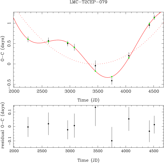
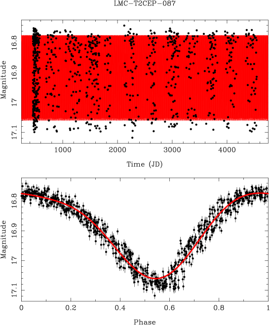
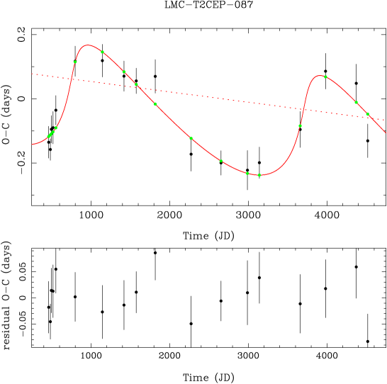
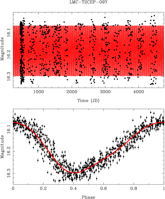
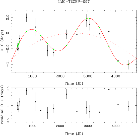
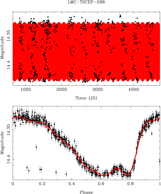
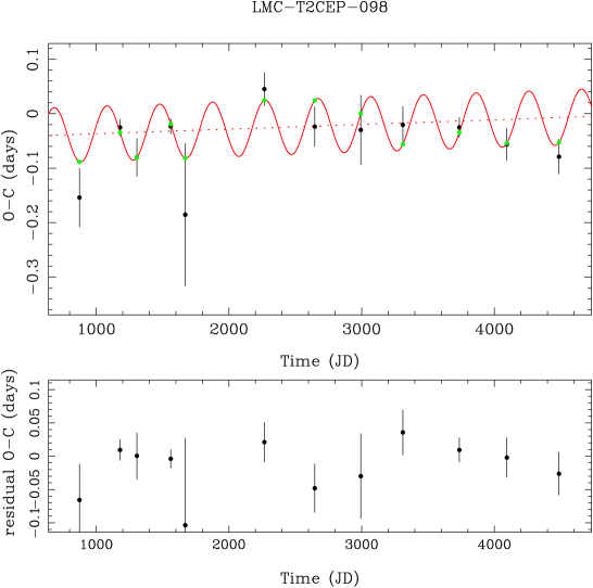
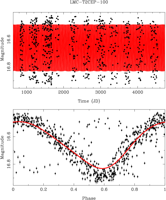
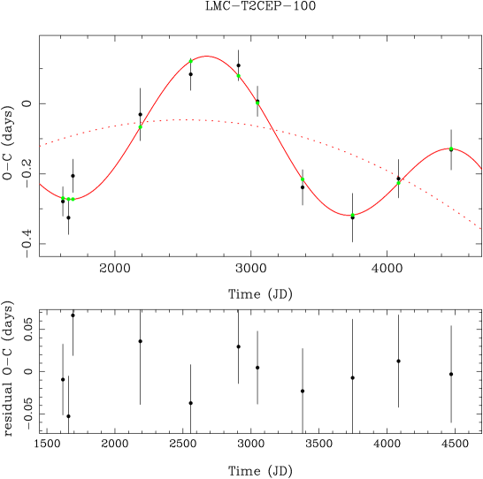
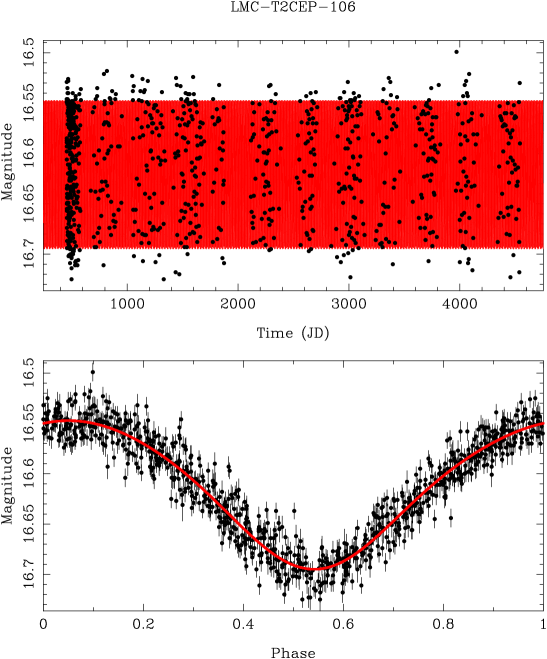
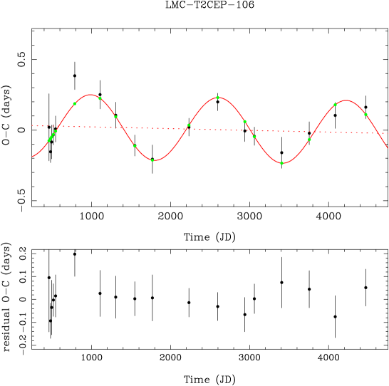
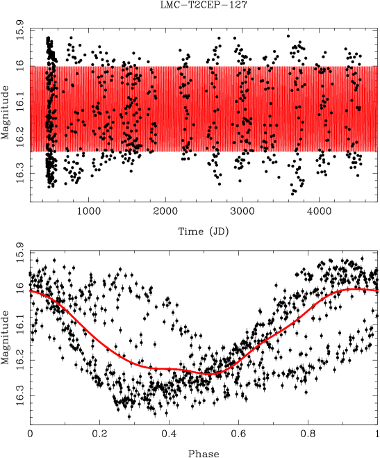
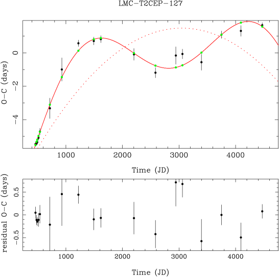
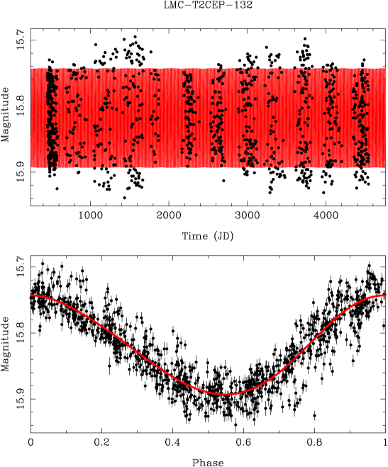
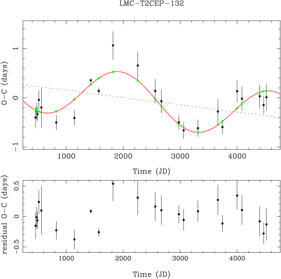
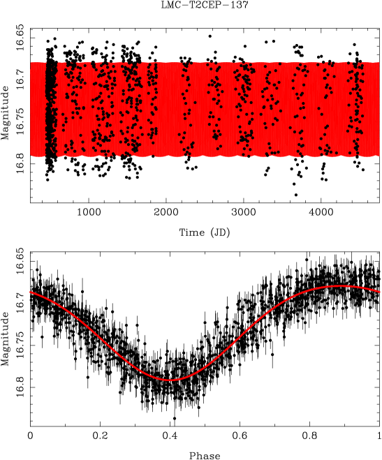
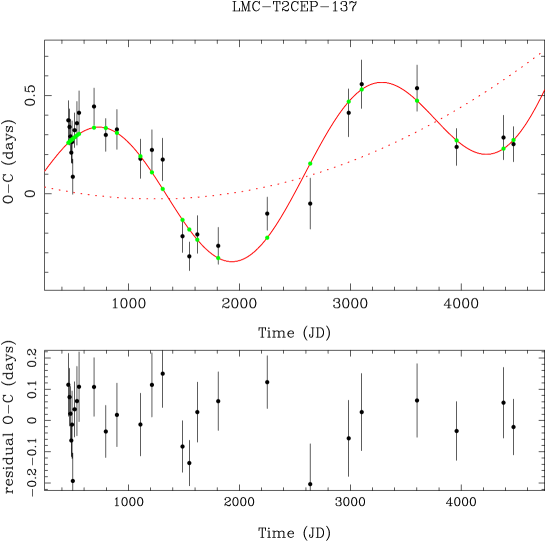
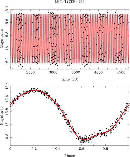
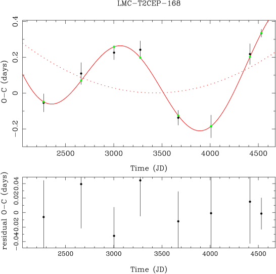
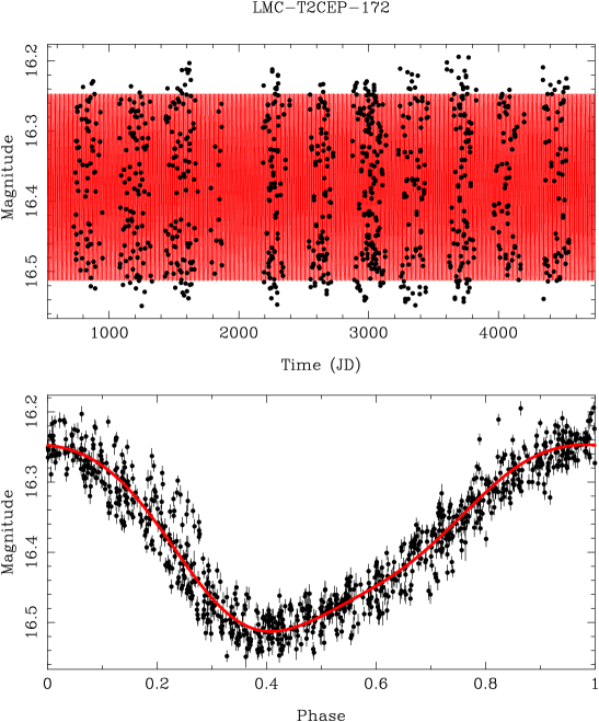
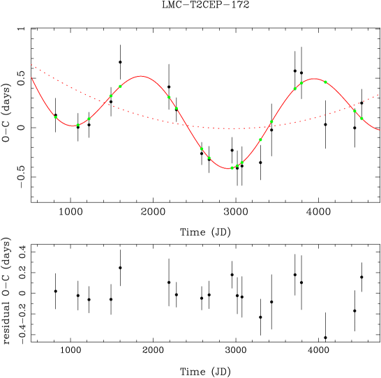
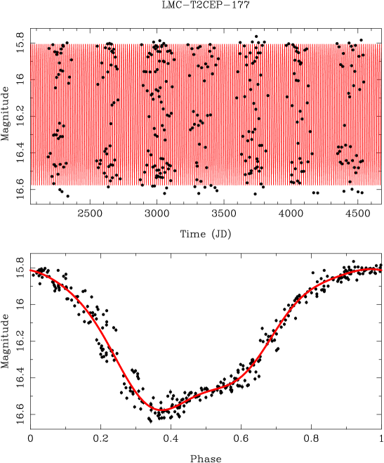
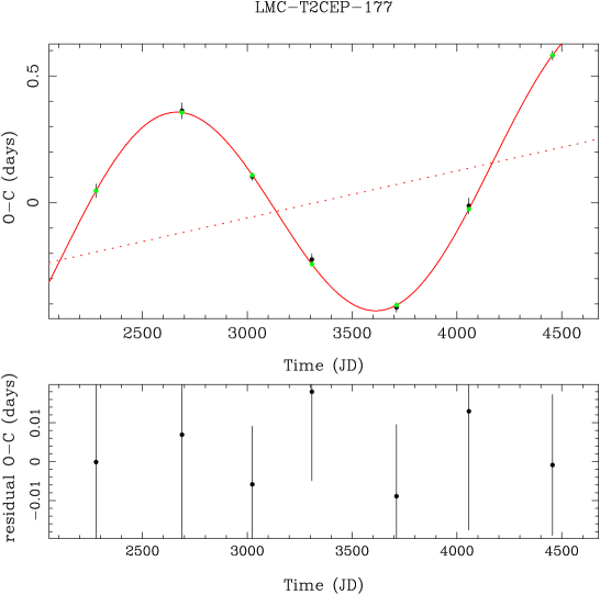
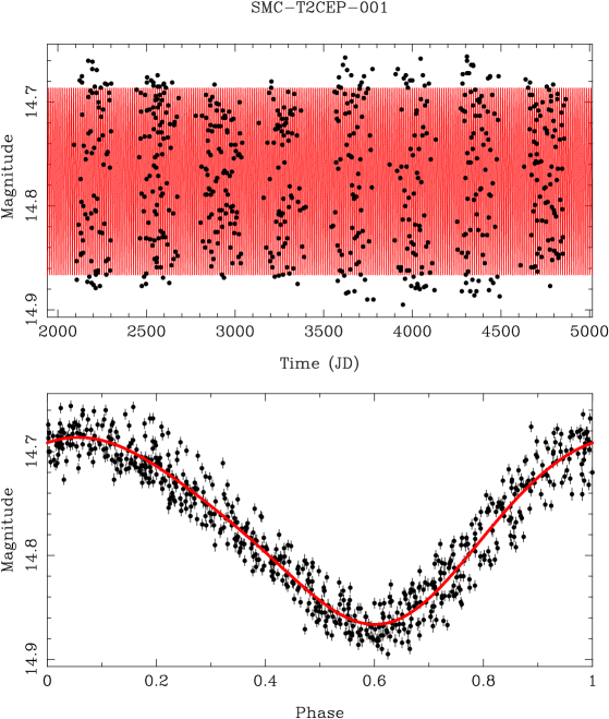
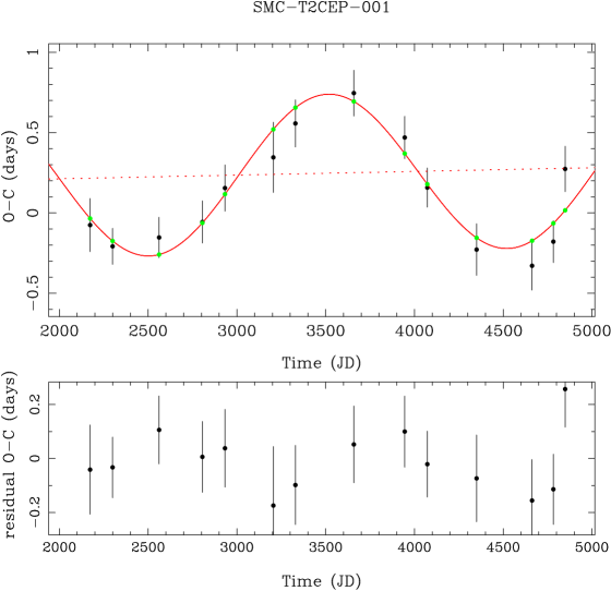
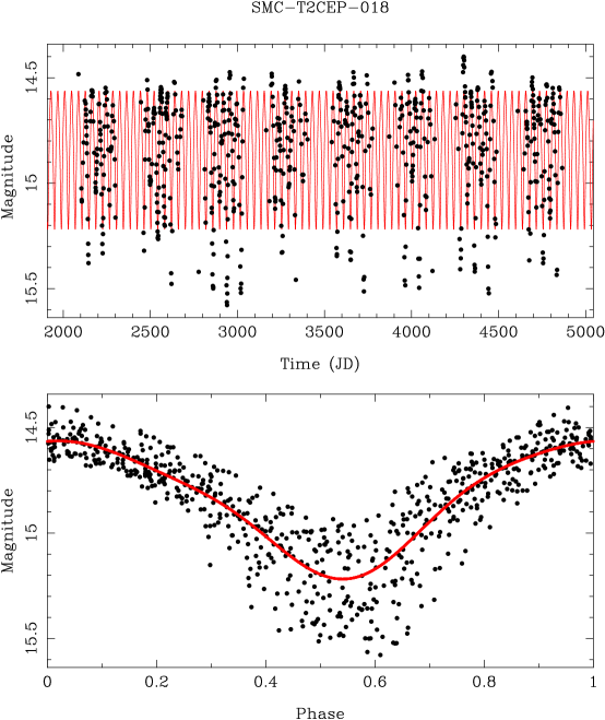
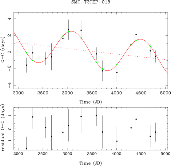
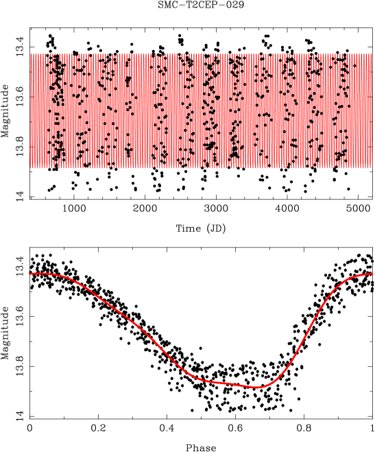
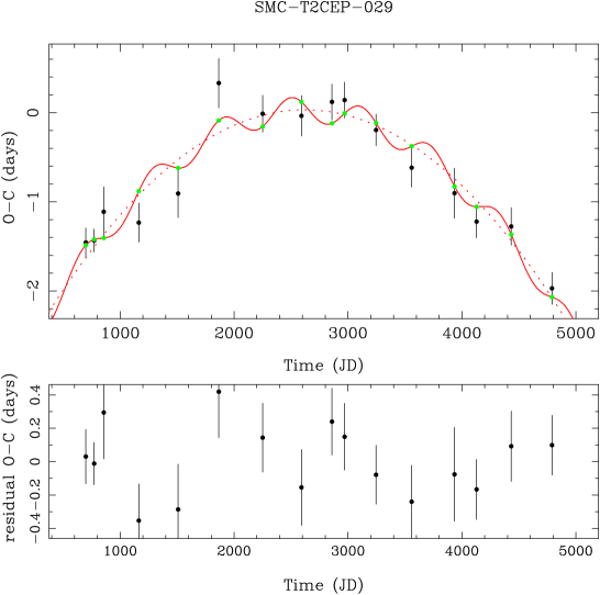
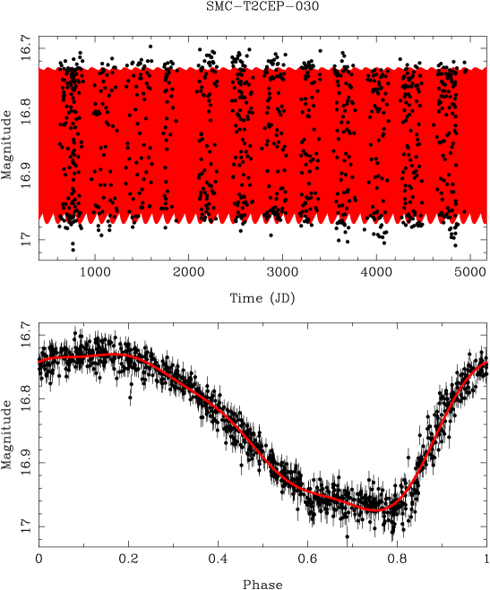
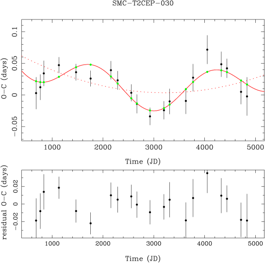
Name	$\dot{P}$	Type	Period	Remarks
	(s/yr)		(d)
LMC-T2CEP-019	$84\pm 6$	pWVir	8.7
LMC-T2CEP-026		WVir	13.6	change in amplitude and period jump at JD $\sim$ 3800
LMC-T2CEP-029	$-10867\pm 594$	RVTau	21.2
LMC-T2CEP-034	$631\pm 33$	WVir	14.9
LMC-T2CEP-037	$236\pm 23$	WVir	6.9
LMC-T2CEP-049	$14.7\pm 1.5$	BLHer	3.2
LMC-T2CEP-072	$1532\pm 160$	WVir	14.5
LMC-T2CEP-074	$-875\pm 91$	WVir	9.0	Binary (P= 1500d) ?
LMC-T2CEP-082	$-7715\pm 1101$	RVTau	35.1	JD $<$ 4200
LMC-T2CEP-099	$505\pm 95$	WVir	15.5	Binary (P= 2300d) ?
LMC-T2CEP-103	$-303\pm 32$	WVir	12.9
LMC-T2CEP-104	$-311\pm 101$	RVTau	24.9
LMC-T2CEP-113	$-57.2\pm 8.5$	BLHer	3.1
LMC-T2CEP-115	$1341\pm 298$	RVTau	25.0
LMC-T2CEP-119	$9078\pm 1751$	RVTau	33.8
LMC-T2CEP-126	$703\pm 80$	WVir	16.3
LMC-T2CEP-135	$2163\pm 450$	RVTau	26.5
LMC-T2CEP-139	$643\pm 86$	WVir	14.8
LMC-T2CEP-143	$-900\pm 70$	WVir	14.6
LMC-T2CEP-146	$704\pm 54$	WVir	10.1
LMC-T2CEP-149		RVTau	42.5	decreasing amplitude and period jump at JD $\sim$ 3800
LMC-T2CEP-152	$-111\pm 15$	WVir	9.3
LMC-T2CEP-155	$158\pm 41$	WVir	6.9
LMC-T2CEP-156	$708\pm 140$	WVir	15.4	alternatively, period jump near JD $\sim$ 3300
LMC-T2CEP-162	$-1947\pm 270$	RVTau	30.4
LMC-T2CEP-170	$-133\pm 32$	WVir	7.7
LMC-T2CEP-182	$244\pm 38$	WVir	8.3
LMC-T2CEP-186	$714\pm 95$	WVir	16.4
LMC-T2CEP-190	$29900\pm 2400$	RVTau	38.6
LMC-T2CEP-191	$-24500\pm 2000$	RVTau	34.3
LMC-T2CEP-201	$153\pm 25$	pWVir	11.0
SMC-ACEP-003	$-2.71\pm 0.20$	ANCEP	0.6
SMC-T2CEP-004	$89.8\pm 7.9$	WVir	6.5
SMC-T2CEP-014	$-442\pm 51$	WVir	13.9	Fit for JD$>$ 1200. Different period before that date ?
SMC-T2CEP-015	$44.0\pm 5.7$	BLHer	2.6
SMC-T2CEP-019		RVTau	40.9	Amplitude variations. Period jump near JD $\sim$ 4000 ?
SMC-T2CEP-025	$196\pm 26$	pWVir	14.2
SMC-T2CEP-032	$-943\pm 69$	WVir	14.2	Binary (P= 1500d) ?
SMC-T2CEP-034		WVir	20.1	Period jump near JD $\sim$ 3050 ?
SMC-T2CEP-038	$11.3\pm 1.9$	pWVir	4.4
SMC-T2CEP-040	$-631\pm 37$	WVir	16.1
SMC-T2CEP-043	$-1121\pm 249$	RVTau	23.7

Figure 4: Light curves and O-C diagrams of the stars showing a significant change in period. The left-hand panel shows the time series (top) and phased light curve (bottom). The right-hand panel shows the O-C diagram (top) and the model and the residuals after subtracting the model (bottom).

Figure 4: Continued.

Figure 4: Continued.

Figure 4: Continued.

Figure 4: Continued.

Table 4: T2C investigated for the LITE with inconclusive results

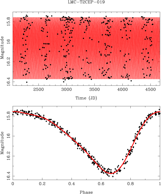
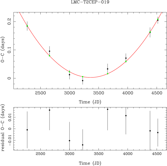
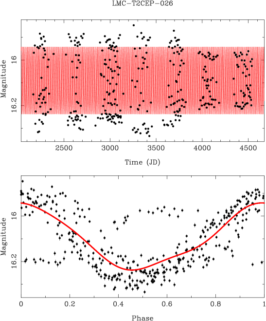
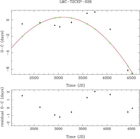
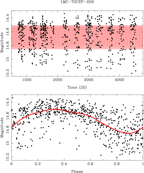
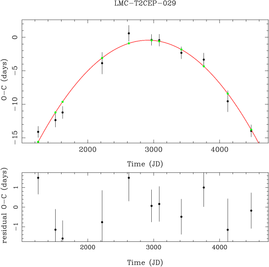
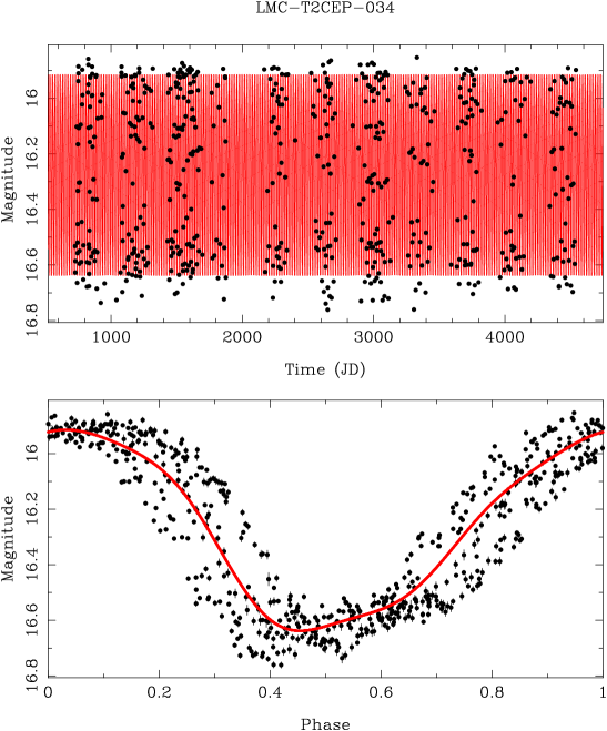
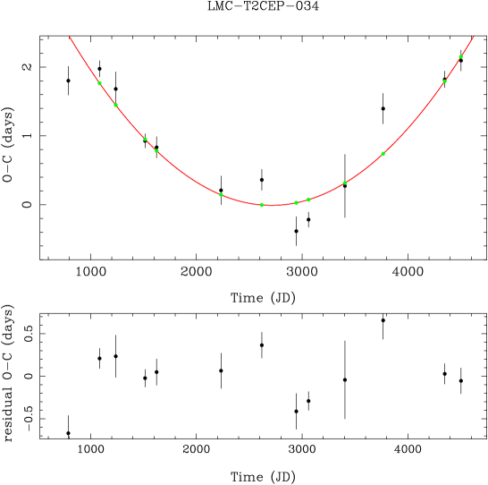
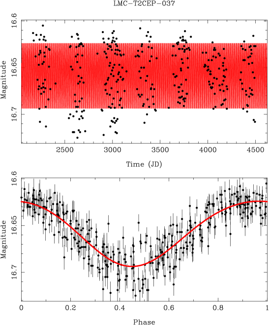
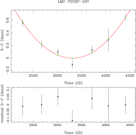
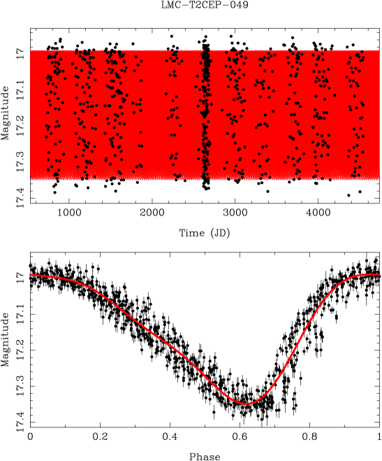
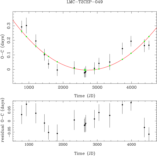
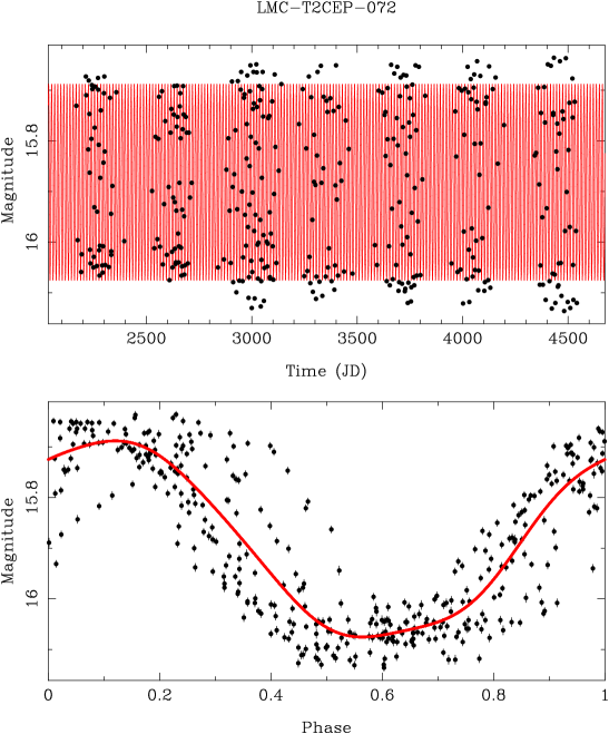
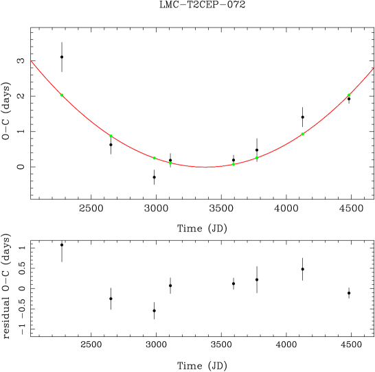
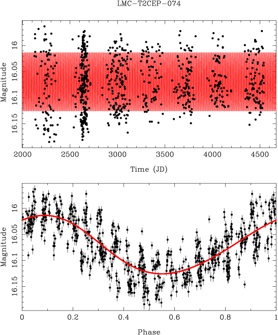
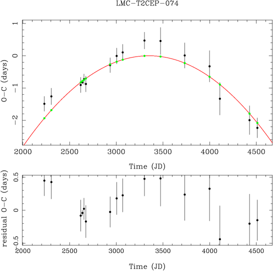
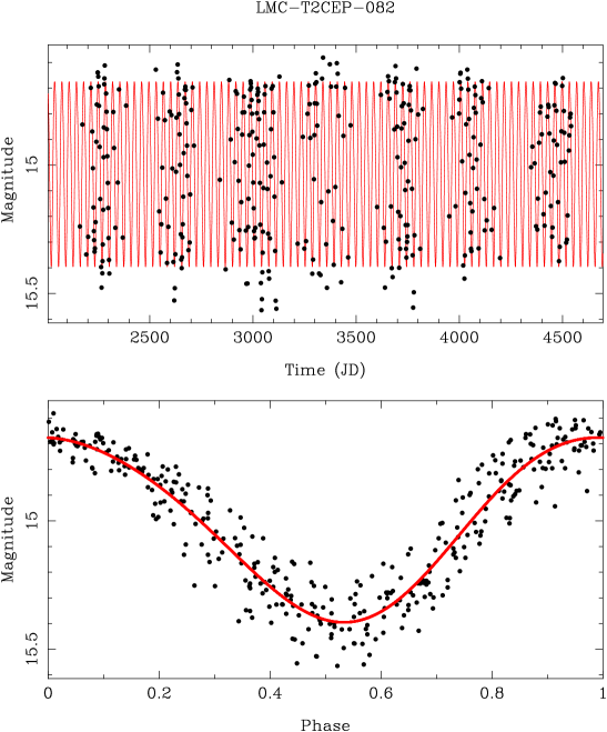
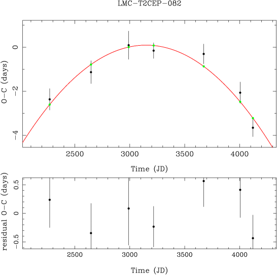
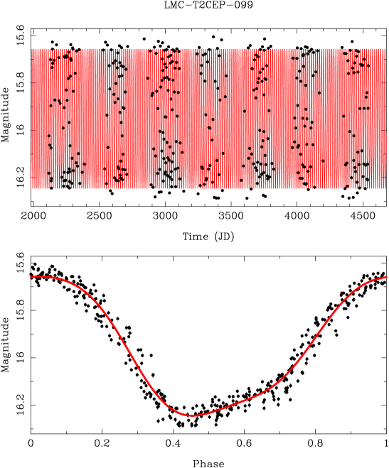
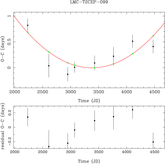
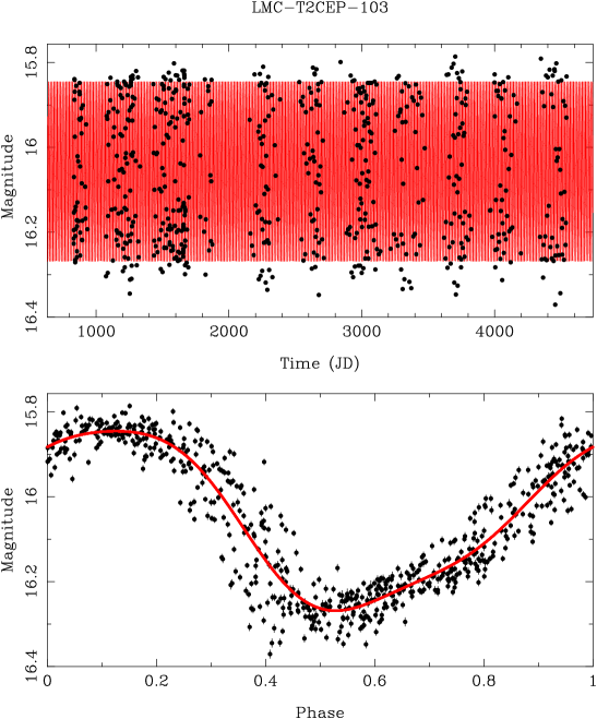
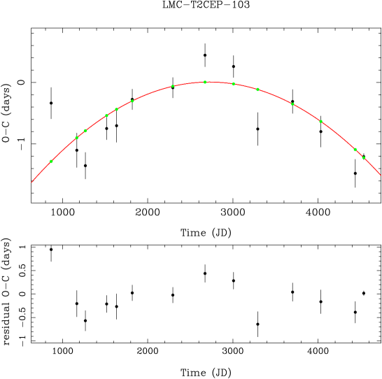
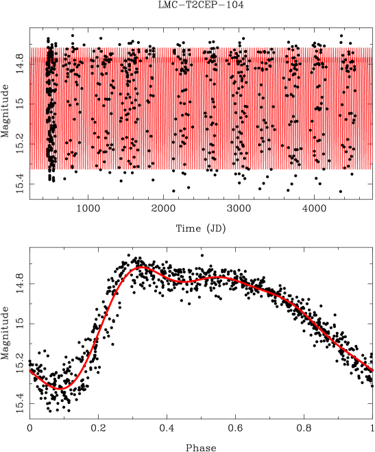
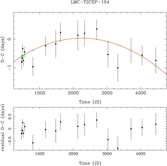
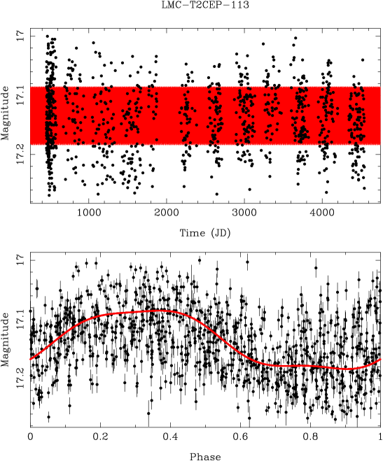
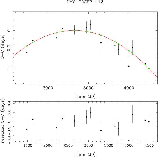
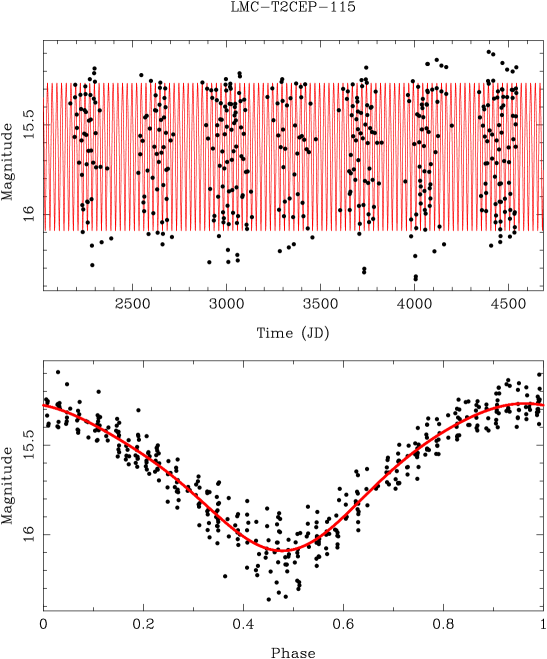
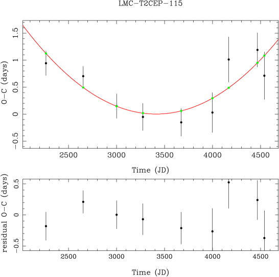
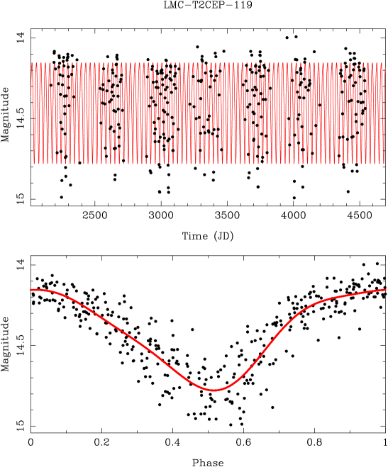
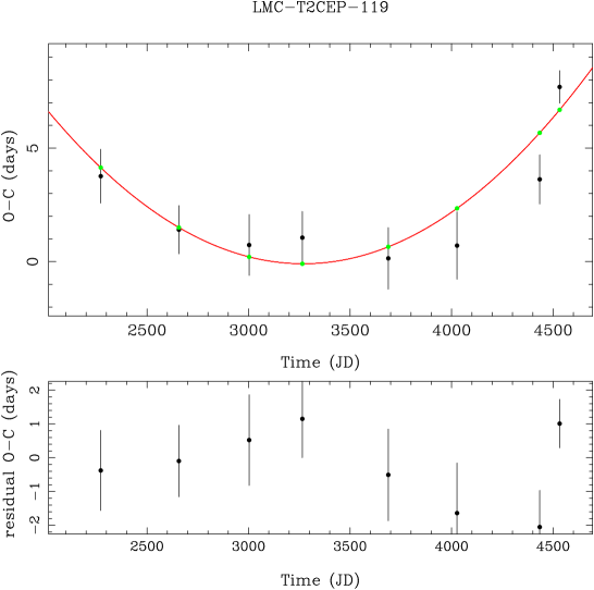
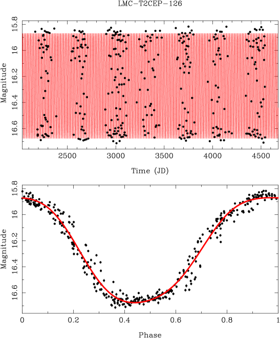
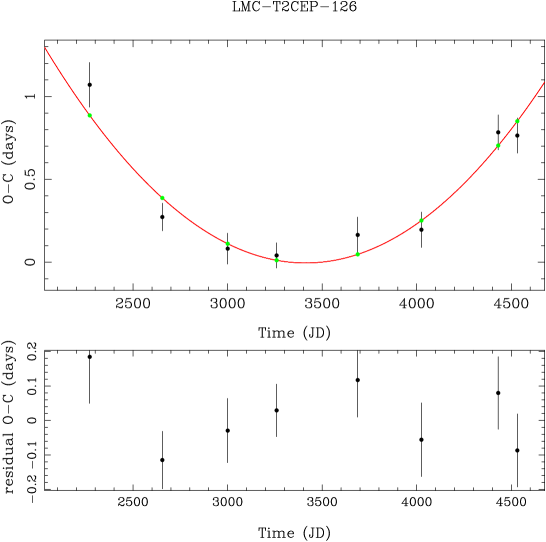
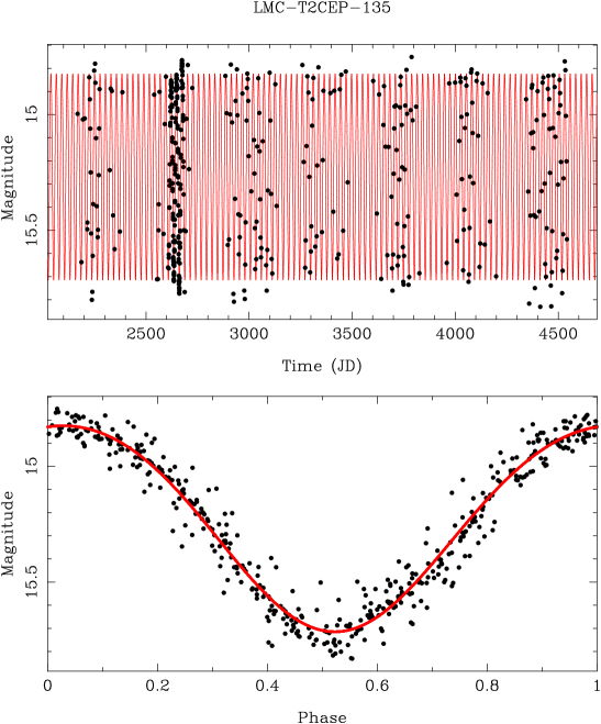
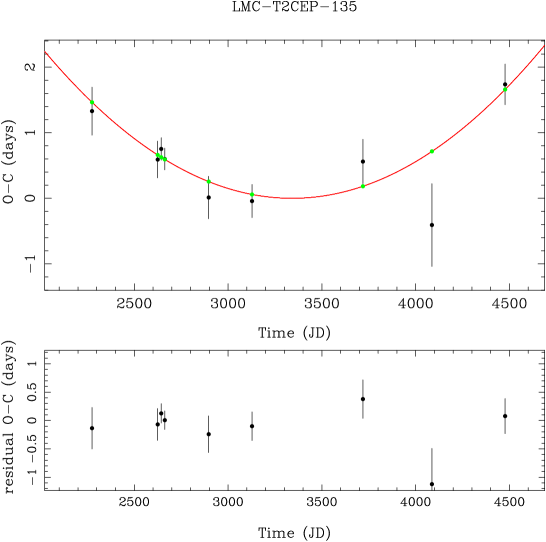
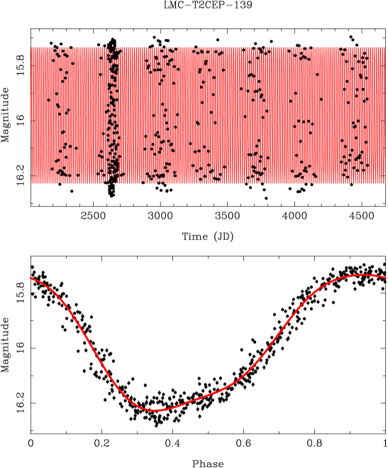
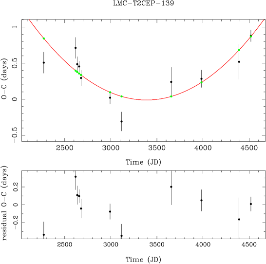
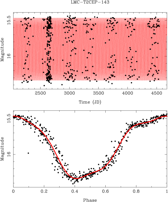
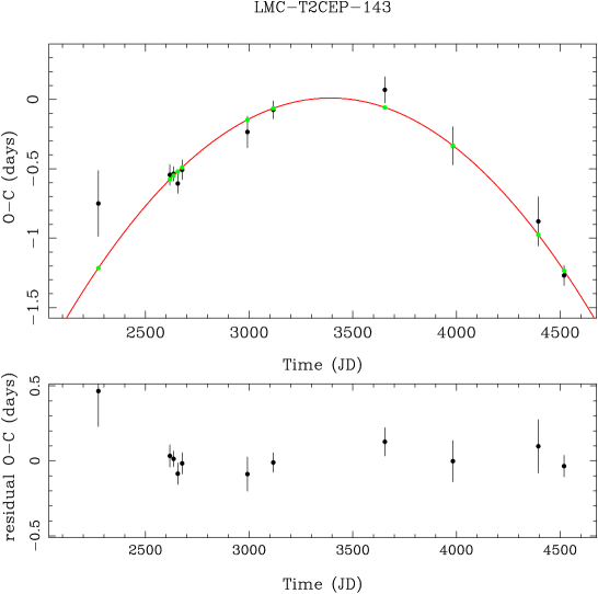
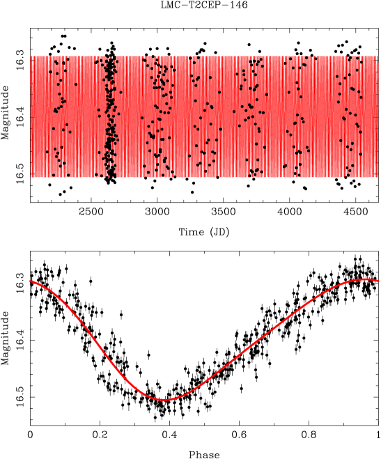
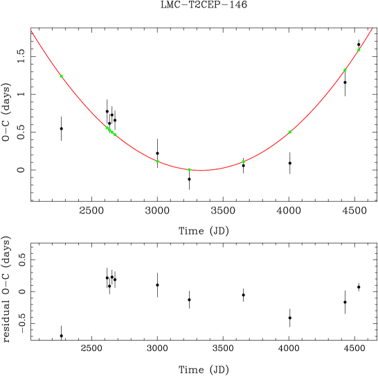
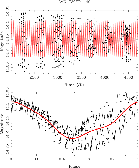
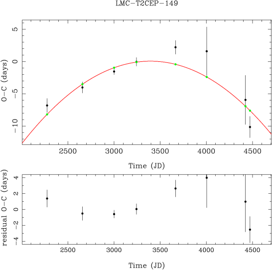
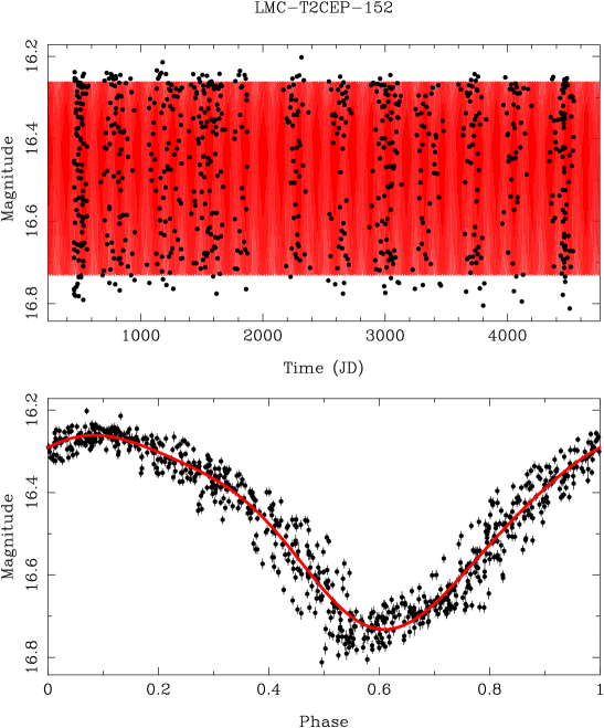
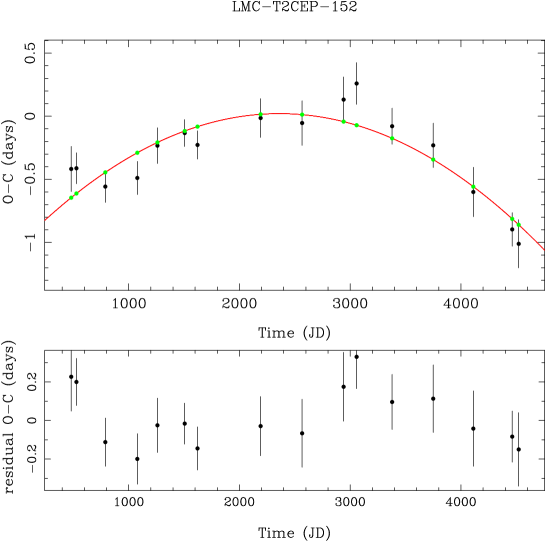
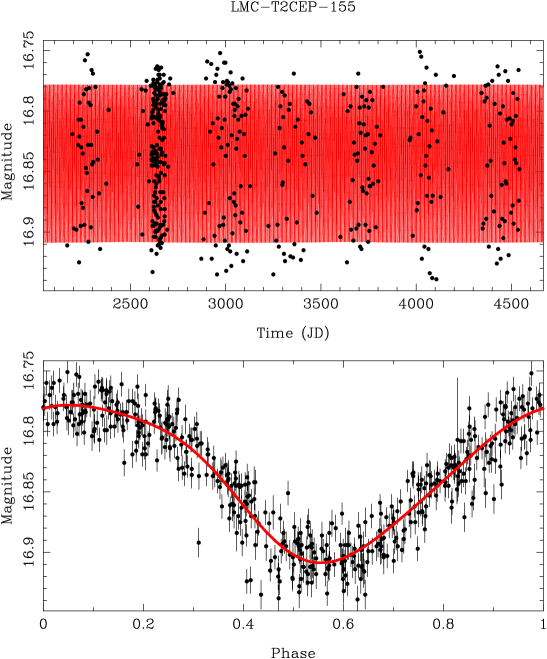
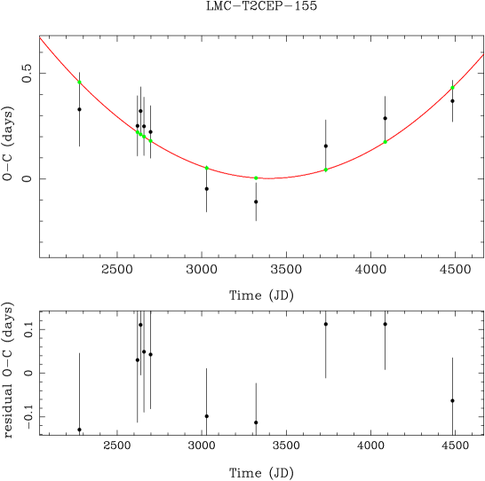
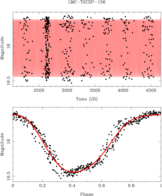
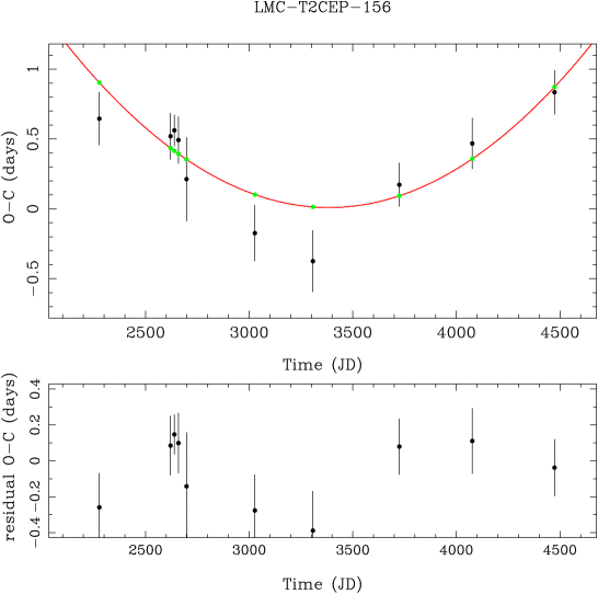
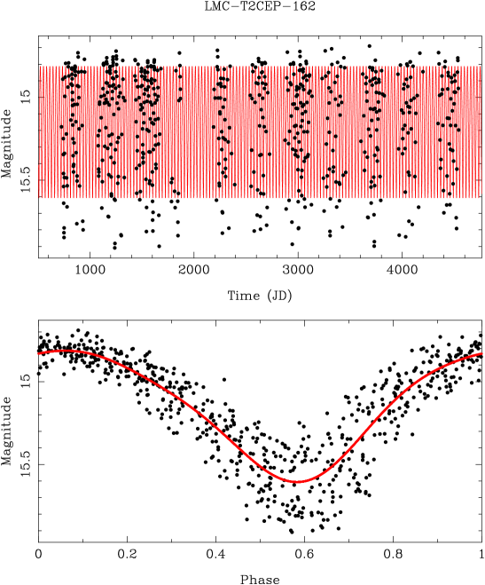
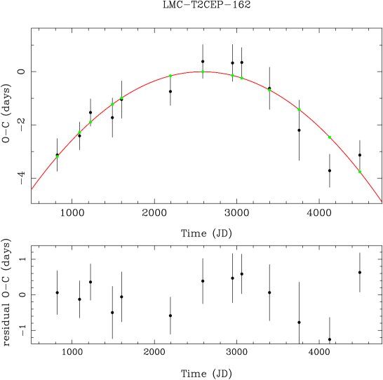
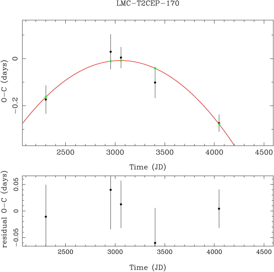
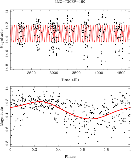
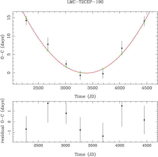
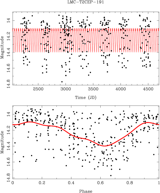
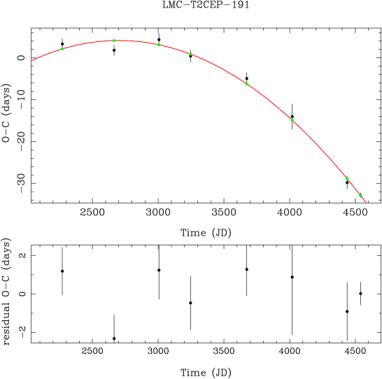
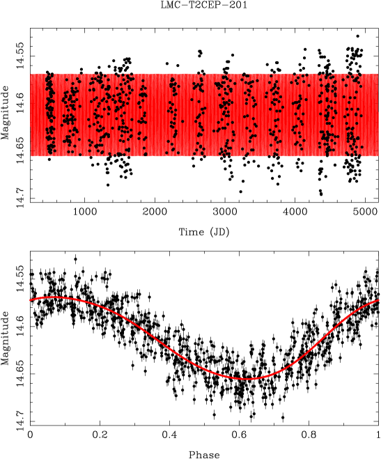
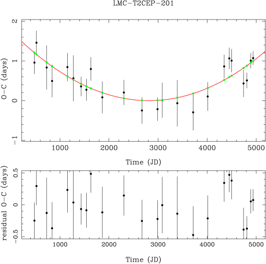
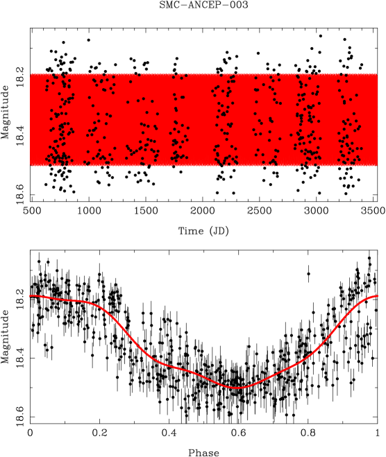
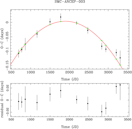
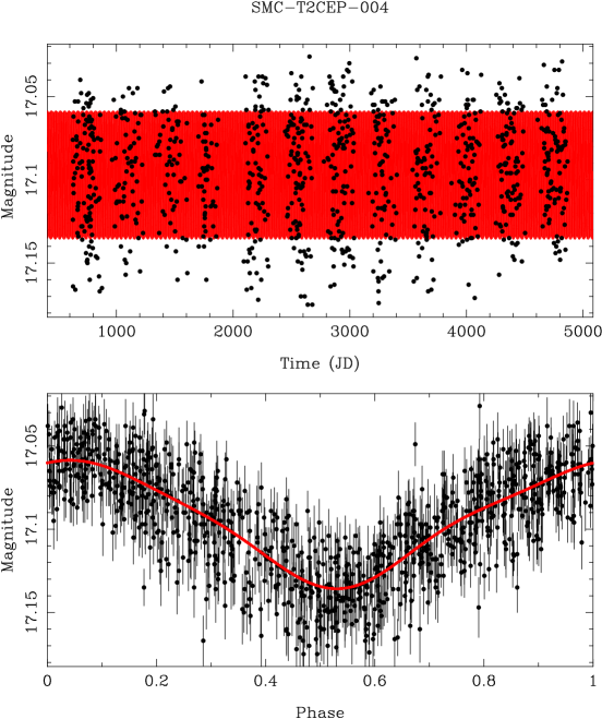
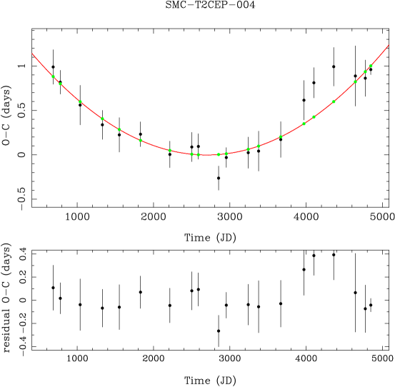
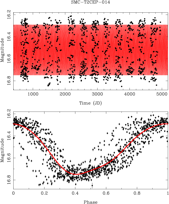
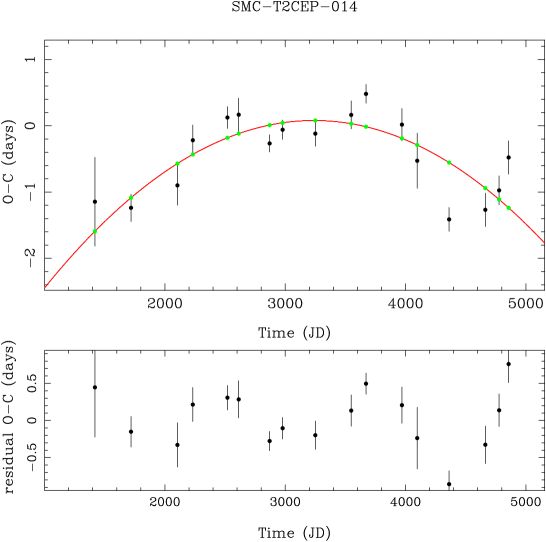
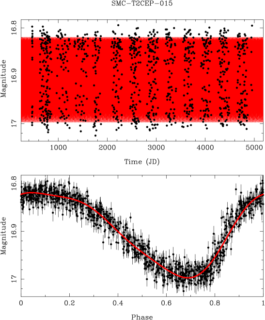
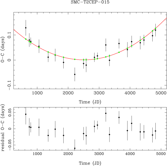
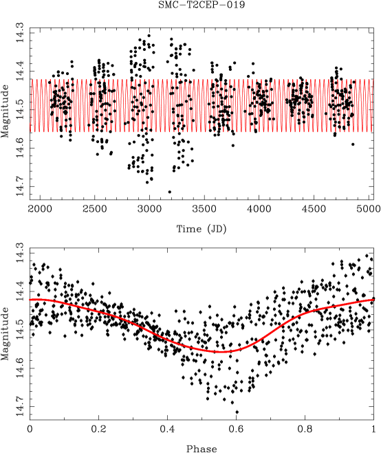
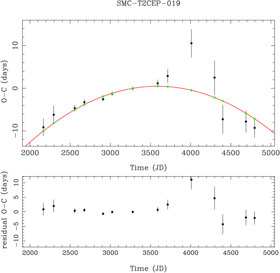
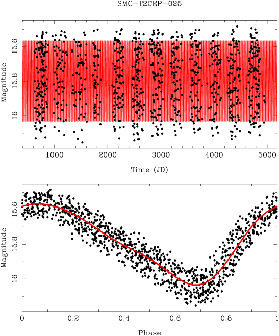
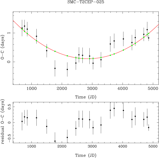
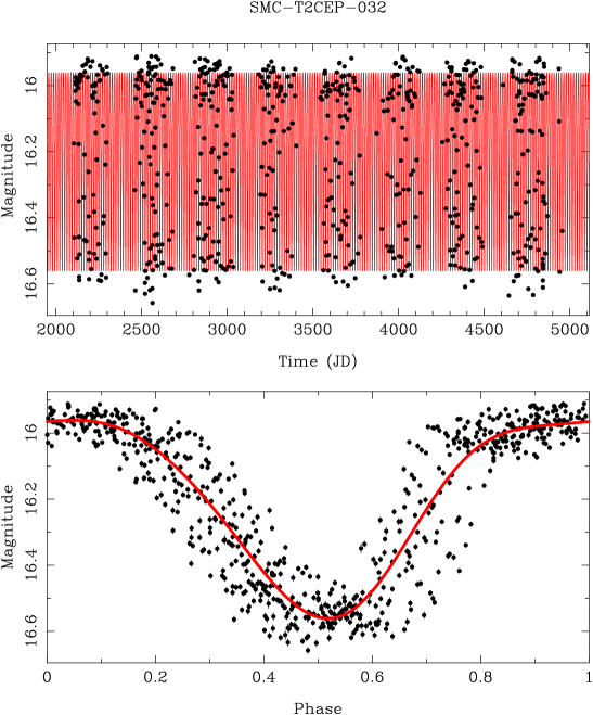
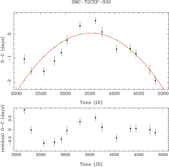
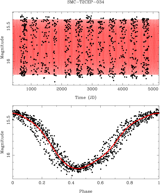
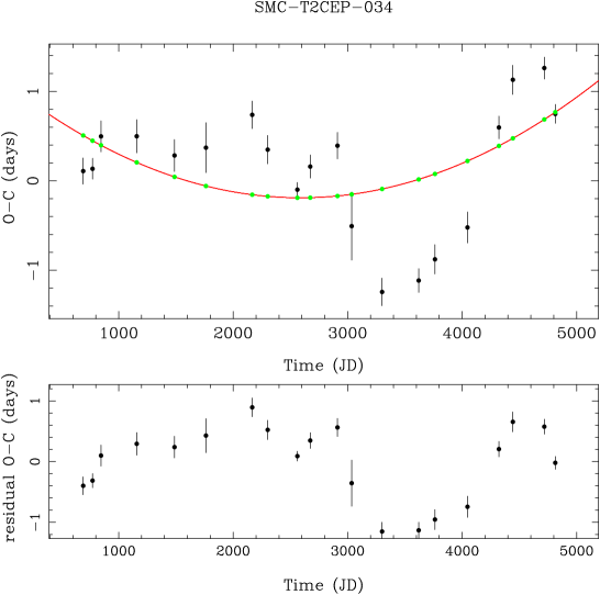
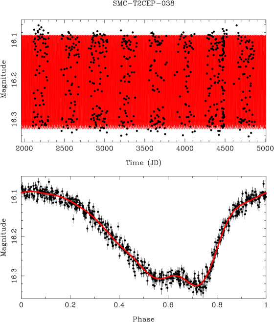
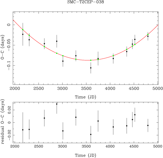
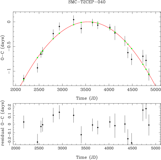
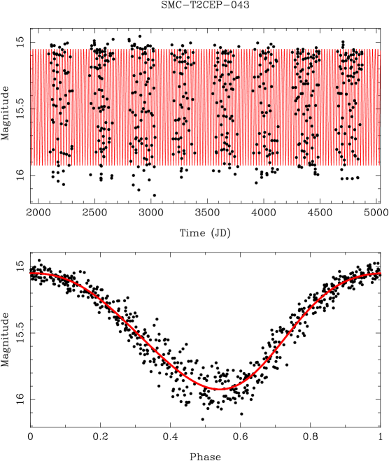
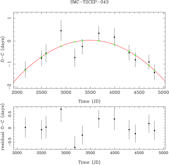
Name	Remarks	Name	Remarks	Name	Remarks
LMC-ACEP-024		LMC-ACEP-058		LMC-ACEP-070
LMC-ACEP-083	$\dot{P}$ ?	LMC-T2CEP-002	$\dot{P}$ ?	LMC-T2CEP-005	$\dot{P}$ ?
LMC-T2CEP-012		LMC-T2CEP-013		LMC-T2CEP-015	$\dot{P}$ ?
LMC-T2CEP-023	known EB	LMC-T2CEP-028		LMC-T2CEP-032
LMC-T2CEP-035		LMC-T2CEP-042		LMC-T2CEP-051	$\dot{P}$ ? Amplitude variations
LMC-T2CEP-052	known EB	LMC-T2CEP-056		LMC-T2CEP-061
LMC-T2CEP-067		LMC-T2CEP-077	claimed EB	LMC-T2CEP-078
LMC-T2CEP-083		LMC-T2CEP-084	known EB	LMC-T2CEP-088
LMC-T2CEP-089		LMC-T2CEP-093	known EB	LMC-T2CEP-101	$\dot{P}$ ?
LMC-T2CEP-108		LMC-T2CEP-117		LMC-T2CEP-129	irregular light curve
LMC-T2CEP-133	$\dot{P}$ ?	LMC-T2CEP-134	binary (P= 2200d) ?	LMC-T2CEP-145
LMC-T2CEP-147		LMC-T2CEP-150		LMC-T2CEP-151
LMC-T2CEP-153		LMC-T2CEP-154	$\dot{P}$ ?	LMC-T2CEP-164
LMC-T2CEP-169		LMC-T2CEP-174		LMC-T2CEP-175	$\dot{P}$ ?
LMC-T2CEP-176	$\dot{P}$ ?	LMC-T2CEP-178	$\dot{P}$ ?	LMC-T2CEP-179	$\dot{P}$ or binary (P= 1800d) ?
LMC-T2CEP-180		LMC-T2CEP-181		LMC-T2CEP-183
LMC-T2CEP-184		LMC-T2CEP-185		LMC-T2CEP-192
LMC-T2CEP-193		LMC-T2CEP-199		LMC-T2CEP-200	known EB
LMC-T2CEP-202		LMC-T2CEP-203
SMC-T2CEP-005	$\dot{P}$ ?	SMC-T2CEP-007		SMC-T2CEP-010
SMC-T2CEP-012		SMC-T2CEP-013	binary (P= 1700d) ?	SMC-T2CEP-020
SMC-T2CEP-023	known EB	SMC-T2CEP-024	Amplitude variations	SMC-T2CEP-028	known EB
SMC-T2CEP-031		SMC-T2CEP-036		SMC-T2CEP-041