KEK-CP-357

OU-HET-928

Chiral behavior of Kπlν𝐾𝜋𝑙𝜈K\!\to\!\pi l\nu decay form factors in lattice QCD with exact chiral symmetry

S. Aokia, G. Cossub, X. Fengc,d, H. Fukayae, S. Hashimotof,g, T. Kanekof,g, J. Noakif and T. Onogie (JLQCD Collaboration) aYukawa Institute for Theoretical Physics, Kyoto University, Kyoto 606-8502, Japan
bSchool of Physics and Astronomy, The University of Edinburgh, Edinburgh EH9 3JZ, United Kingdom
cPhysics Department, Columbia University, New York, NY 10027, USA
dSchool of Physics, Peking University, Beijing 100871, China
eDepartment of Physics, Osaka University, Osaka 560-0043, Japan
fHigh Energy Accelerator Research Organization (KEK), Ibaraki 305-0801, Japan
gSchool of High Energy Accelerator Science, SOKENDAI (The Graduate University for Advanced Studies), Ibaraki 305-0801, Japan
Abstract

We calculate the form factors of the Kπlν𝐾𝜋𝑙𝜈K\!\to\!\pi l\nu semileptonic decays in three-flavor lattice QCD, and study their chiral behavior as a function of the momentum transfer and the Nambu-Goldstone boson masses. Chiral symmetry is exactly preserved by using the overlap quark action, which enables us to directly compare the lattice data with chiral perturbation theory (ChPT). We generate gauge ensembles at a lattice spacing of 0.11 fm with four pion masses covering 290 – 540 MeV and a strange quark mass mssubscript𝑚𝑠m_{s} close to its physical value. By using the all-to-all quark propagator, we calculate the vector and scalar form factors with high precision. Their dependence on mssubscript𝑚𝑠m_{s} and the momentum transfer is studied by using the reweighting technique and the twisted boundary conditions for the quark fields. We compare the results for the semileptonic form factors with ChPT at next-to-next-to leading order in detail. While many low-energy constants appear at this order, we make use of our data of the light meson electromagnetic form factors in order to control the chiral extrapolation. We determine the normalization of the form factors as f+(0)=0.9636(36)()35+57f_{+}(0)\!=\!0.9636(36)\left({}^{+57}_{-35}\right), and observe reasonable agreement of their shape with experiment.

I Introduction

The kaon semileptonic decays Kπlν𝐾𝜋𝑙𝜈K\!\to\!\pi l\nu provide a precise determination of the Cabibbo-Kobayashi-Maskawa (CKM) matrix element |Vus|subscript𝑉𝑢𝑠|V_{us}|. The decay rate is given as

Γ(Kπlν)Γ𝐾𝜋𝑙𝜈\displaystyle\Gamma(K\!\to\!\pi l\nu) =\displaystyle= GF2MK5192π3C2SEW(1+δEM+δSU(2))2I|Vus|2f+(0)2,superscriptsubscript𝐺𝐹2superscriptsubscript𝑀𝐾5192superscript𝜋3superscript𝐶2subscript𝑆EWsuperscript1subscript𝛿EMsubscript𝛿𝑆𝑈22𝐼superscriptsubscript𝑉𝑢𝑠2subscript𝑓superscript02\displaystyle\frac{G_{F}^{2}M_{K}^{5}}{192\pi^{3}}C^{2}S_{\rm EW}\left(1+\delta_{\rm EM}+\delta_{SU(2)}\right)^{2}I|V_{us}|^{2}f_{+}(0)^{2}, (1)

where GFsubscript𝐺𝐹G_{F} is the Fermi constant, the Clebsch-Gordan coefficient C𝐶C is 1 (1/2121/\sqrt{2}) for the K0superscript𝐾0K^{0} (K±superscript𝐾plus-or-minusK^{\pm}) decay, and I𝐼I represents the phase space integral. We denote the short-distance electroweak, long-distance electromagnetic (EM), and isospin-breaking corrections by SEWsubscript𝑆EWS_{\rm EW}, δEMsubscript𝛿EM\delta_{\rm EM} and δSU(2)subscript𝛿𝑆𝑈2\delta_{SU(2)}, respectively.

The vector form factor f+(t)subscript𝑓𝑡f_{+}(t) is defined from relevant hadronic matrix element

π(p)|Vμ|K(p)quantum-operator-product𝜋superscript𝑝subscript𝑉𝜇𝐾𝑝\displaystyle\langle\pi({p^{\prime}})|V_{\mu}|K(p)\rangle =\displaystyle= (p+p)μf+(t)+(pp)μf(t),subscript𝑝superscript𝑝𝜇subscript𝑓𝑡subscript𝑝superscript𝑝𝜇subscript𝑓𝑡\displaystyle(p+{p^{\prime}})_{\mu}f_{+}(t)+(p-{p^{\prime}})_{\mu}f_{-}(t), (2)

where t=(pp)2𝑡superscriptsuperscript𝑝𝑝2t\!=\!({p^{\prime}}-p)^{2} is the momentum transfer. Instead of f(t)subscript𝑓𝑡f_{-}(t), the scalar form factor

f0(t)subscript𝑓0𝑡\displaystyle f_{0}(t) =\displaystyle= f+(t)+tMK2Mπ2f(t)subscript𝑓𝑡𝑡superscriptsubscript𝑀𝐾2superscriptsubscript𝑀𝜋2subscript𝑓𝑡\displaystyle f_{+}(t)+\frac{t}{M_{K}^{2}-M_{\pi}^{2}}f_{-}(t) (3)

has been widely used in phenomenological analyses of the semileptonic decays. By definition, the normalizations of the vector and scalar form factors coincide with each other at the zero momentum transfer t=0𝑡0t\!=\!0,

f+(0)=f0(0).subscript𝑓0subscript𝑓00\displaystyle f_{+}(0)=f_{0}(0). (4)

The Ademollo-Gatto theorem Behrends-Sirlin ; Ademollo-Gatto states that SU(3) breaking effects are suppressed as f+(0)=1+O((mlms)2)subscript𝑓01𝑂superscriptsubscript𝑚𝑙subscript𝑚𝑠2f_{+}(0)\!=\!1+O((m_{l}-m_{s})^{2}), where ml=(mu+md)/2subscript𝑚𝑙subscript𝑚𝑢subscript𝑚𝑑2m_{l}\!=\!(m_{u}+m_{d})/2 and m{u,d,s}subscript𝑚𝑢𝑑𝑠m_{\{u,d,s\}} represent the masses of up, down and strange quarks. The normalization f+(0)subscript𝑓0f_{+}(0) has been therefore used as an important input to determine |Vus|subscript𝑉𝑢𝑠|V_{us}| through the decay rate (1).

Since the form factors describe effects due to the strong interaction at low energy, a precise calculation of f+(0)subscript𝑓0f_{+}(0) needs a non-perturbative method to study QCD. A target accuracy is 1less-than-or-similar-toabsent1\lesssim 1 %, because other experimental and theoretical inputs have been determined with a similar or even better accuracy CKM16:Moulson ; CKM16:WG1 . Lattice QCD is the only known method to calculate the form factors with controlled and systematically-improvable accuracy.

The phase space integral I𝐼I encodes information about the shape of the form factors, namely their t𝑡t dependence. The current determination of |Vus|subscript𝑉𝑢𝑠|V_{us}| employs a precise estimate of I𝐼I obtained from experimental data. A lattice study of the form factor shape and comparison with experiments can examine the reliability of the numerical lattice determination of the normalization f+(0)subscript𝑓0f_{+}(0). We note that new physics can modify not only the normalization but also the shape, which may therefore provide a different probe of new physics if both theoretical and experimental data become sufficiently accurate in the future.

Lattice calculation of f+(0)subscript𝑓0f_{+}(0) has become mature FLAG3 ; CKM16:Simula ; CKM16:WG1 by realistic simulations at reasonably small pion masses and lattice spacings. The so-called twisted boundary condition TBC enables us to simulate near the reference point t0similar-to-or-equals𝑡0t\!\simeq\!0. Although recent lattice studies Kl3:Nf3:FNAL+MILC ; Kl3:Nf3:RBC/UKQCD ; Kl3:Nf4:FNAL+MILC ; Kl3:Nf4:ETM have achieved sub-% accuracy, more independent calculations are welcome to establish the lattice estimate with such a high precision. A detailed study of the form factor shape based on the next-to-leading order (NLO) chiral perturbation theory (ChPT) ChPT:SU2:NLO ; ChPT:SU3:NLO ; KFF:ChPT:SU3:NLO and model independent parametrization z-param ; shape:disp:vector ; shape:disp:scalar is also available Kl3:Nf4:ETM .

A recent trend of precision calculations is to directly simulate physical quark masses at t=0𝑡0t\!=\!0. In this study, we take a different approach based on our large-scale simulations with exact chiral symmetry JLQCD:overlap:summary . By exploiting exact symmetry, we directly compare our lattice data with next-to-next-to-leading order (NNLO) ChPT KFF:weak:ChPT:SU3:NNLO:PS ; KFF:weak:ChPT:SU3:NNLO:BT , and determine the normalization f+(0)subscript𝑓0f_{+}(0), relevant low-energy constants (LECs) in the ChPT Lagrangian, and study the form factor shape. We note that chiral symmetry is explicitly violated with conventional lattice actions. The explicit violation makes the direct comparison between lattice QCD and NNLO ChPT difficult because of modified functional form of the ChPT formulae and additional unknown LECs.

For a rigorous comparison with ChPT, we calculate the form factors with high precision by using the so-called all-to-all quark propagator A2A:SESAM ; A2A:TrinLat . The strange quark mass dependence and the form factor shape near the reference point t=0𝑡0t\!=\!0 are studied by employing the reweighting technique reweight:1 ; reweight:2 and the twisted boundary conditions, respectively. While many unknown LECs appear at NNLO, we control the chiral extrapolation by making use of our lattice data of the light meson EM form factors obtained in Ref. EMFF:JLQCD:Nf3:RG+Ovr . We also employ a linear combination of f0subscript𝑓0f_{0} and the decay constant ratio FK/Fπsubscript𝐹𝐾subscript𝐹𝜋F_{K}/F_{\pi} KFF:weak:ChPT:SU3:NNLO:BT , which has a reduced number of the LECs. Our preliminary analyses have been reported in Refs. Lat10:JLQCD:Kaneko ; Lat11:JLQCD:Kaneko ; Lat12:JLQCD:Kaneko ; Lat15:JLQCD:Kaneko .

This paper is organized as follows. In Sec. II, we introduce our method to generate our gauge ensembles and to calculate relevant meson correlators. The kaon semileptonic form factors are extracted at our simulation points in Sec. III. Section IV details comparison with NNLO ChPT to study the chiral behavior of the form factors, and summarizes the numerical results for the normalization, shape and relevant LECs. We summarize our conclusions in Sec. V.

II Simulation method

II.1 Configuration generation

We simulate Nf=2+1subscript𝑁𝑓21N_{f}\!=\!2+1 QCD using the overlap quark action Overlap:NN ; Overlap:N defined by the Dirac operator

D(mq)𝐷subscript𝑚𝑞\displaystyle D(m_{q}) =\displaystyle= (1mq2m0)D(0)+mq,1subscript𝑚𝑞2subscript𝑚0𝐷0subscript𝑚𝑞\displaystyle\left(1-\frac{m_{q}}{2m_{0}}\right)D(0)+m_{q}, (5)

where mqsubscript𝑚𝑞m_{q} represents the quark mass, and

D(0)𝐷0\displaystyle D(0) =\displaystyle= m0(1+γ5sgn[HW(m0)])subscript𝑚01subscript𝛾5sgndelimited-[]subscript𝐻Wsubscript𝑚0\displaystyle m_{0}\left(1+\gamma_{5}\,{\rm sgn}\left[H_{\rm W}(-m_{0})\right]\right) (6)

is the overlap-Dirac operator in the massless limit. The parameter m0subscript𝑚0m_{0} for the Hermitian Wilson-Dirac operator HWsubscript𝐻𝑊H_{W} is set to m0=1.6subscript𝑚01.6m_{0}\!=\!1.6 from our study of the locality of D𝐷D Prod_Run:JLQCD:Nf2:RG+Ovr . Numerical simulations are remarkably accelerated by modifying the Iwasaki gauge action Iwasaki with an auxiliary Boltzmann weight exW:Vranas ; exW+extmW:JLQCD

ΔWsubscriptΔW\displaystyle\Delta_{\rm W} =\displaystyle= det[HW(m0)2]det[HW(m0)2+μ2](μ=0.2)delimited-[]subscript𝐻Wsuperscriptsubscript𝑚02delimited-[]subscript𝐻Wsuperscriptsubscript𝑚02superscript𝜇2𝜇0.2\displaystyle\frac{\det[H_{\rm W}(-m_{0})^{2}]}{\det[H_{\rm W}(-m_{0})^{2}+\mu^{2}]}\hskip 14.22636pt(\mu=0.2) (7)

and by simulating the trivial topological sector. The effect of the fixed global topology can be considered as a finite volume effect suppressed by the inverse lattice volume fixed_Q:AFHO . In fact, the effect turns out to be small in our previous study of the pion EM form factor on similar and even smaller lattice volumes PFF:JLQCD:Nf2:RG+Ovr ; EMFF:JLQCD:Nf3:RG+Ovr . We also note that local topological excitations are active in our gauge ensembles. Indeed, the topological susceptibility calculated in our simulations is nicely consistent with the prediction of ChPT chi_t:JLQCD .

The lattice spacing a𝑎a determined from the ΩΩ\Omega baryon mass is 0.112(1)0.11210.112(1) fm with our choice of the gauge coupling β=6/g2=2.30𝛽6superscript𝑔22.30\beta\!=6/g^{2}\!=\!2.30. We simulate four values of the degenerate up and down quark masses mlsubscript𝑚𝑙m_{l}. The bare masses are 0.015, 0.025, 0.035 and 0.050 in lattice units, and cover a range of Mπ290similar-tosubscript𝑀𝜋290M_{\pi}\!\sim\!290 – 540 MeV. The gauge ensembles are generated at a strange quark mass ms=0.080subscript𝑚𝑠0.080m_{s}\!=\!0.080, close to its physical value ms,phys=0.081subscript𝑚𝑠phys0.081m_{s,\rm phys}\!=\!0.081. The mssubscript𝑚𝑠m_{s} dependence of the form factors is studied by calculating them at a different ms(=0.060)annotatedsubscript𝑚𝑠absent0.060m_{s}(=\!0.060) using the reweighting technique reweight:1 ; reweight:2 .

The spatial lattice size is set to Ns=L/a=24subscript𝑁𝑠𝐿𝑎24N_{s}\!=\!L/a\!=\!24 or 16 depending on mlsubscript𝑚𝑙m_{l}, so that a condition MπL4greater-than-or-equivalent-tosubscript𝑀𝜋𝐿4M_{\pi}L\gtrsim 4 is satisfied to control finite volume effects. The temporal lattice size is fixed to Nt=T/a=48subscript𝑁𝑡𝑇𝑎48N_{t}\!=\!T/a\!=\!48. The statistics are 2,500 HMC trajectories at each simulation point (ml,ms)subscript𝑚𝑙subscript𝑚𝑠(m_{l},m_{s}). We estimate the statistical error by the jackknife method with a bin size of 50 trajectories. Our simulation parameters are summarized in Table 1.

Table 1: Simulation parameters. Meson masses, Mπsubscript𝑀𝜋M_{\pi} and MKsubscript𝑀𝐾M_{K}, are in units of MeV.
lattice mlsubscript𝑚𝑙m_{l} mssubscript𝑚𝑠m_{s} Mπsubscript𝑀𝜋M_{\pi} MKsubscript𝑀𝐾M_{K} θ𝜃\theta
163×48superscript1634816^{3}\!\times\!48 0.050 0.080 540(3) 617(4) 0.00, 0.40, 0.96, 1.60
163×48superscript1634816^{3}\!\times\!48 0.035 0.080 453(4) 578(4) 0.00, 0.60, 1.28, 1.76
243×48superscript2434824^{3}\!\times\!48 0.025 0.080 379(2) 548(3) 0.00, 1.68, 2.64
243×48superscript2434824^{3}\!\times\!48 0.015 0.080 293(2) 518(1) 0.00, 1.68, 2.64
163×48superscript1634816^{3}\!\times\!48 0.050 0.060 540(4) 567(4) 0.00, 0.40, 0.96, 1.60
163×48superscript1634816^{3}\!\times\!48 0.035 0.060 451(6) 524(5) 0.00, 0.60, 1.28, 1.76
243×48superscript2434824^{3}\!\times\!48 0.025 0.060 378(7) 492(7) 0.00, 1.68, 2.64
243×48superscript2434824^{3}\!\times\!48 0.015 0.060 292(3) 459(4) 0.00, 1.68, 2.64

II.2 Calculation of meson correlators

We calculate the three-point functions of the kaon and pion

Cμ,ϕϕPQ(Δx4,Δx4;𝐩,𝐩)subscriptsuperscript𝐶𝑃𝑄𝜇italic-ϕsuperscriptitalic-ϕΔsubscript𝑥4Δsuperscriptsubscript𝑥4𝐩superscript𝐩\displaystyle C^{PQ}_{\mu,\phi\phi^{\prime}}({\Delta x_{4}},{\Delta x_{4}^{\prime}};{\bf p},{\bf p}^{\prime}) =\displaystyle= 1Ntx4=1Nt𝐱,𝐱,𝐱′′𝒪Q,ϕ(𝐱′′,x4+Δx4+Δx4;𝐩)\displaystyle\frac{1}{N_{t}}\sum_{x_{4}=1}^{N_{t}}\sum_{{\bf x},{{\bf x}^{\prime}},{{\bf x}^{\prime\prime}}}\langle{{\mathcal{O}}}_{Q,\phi^{\prime}}({{\bf x}^{\prime\prime}},x_{4}+{\Delta x_{4}}+{\Delta x_{4}^{\prime}};{{\bf p}^{\prime}}) (8)
×Vμ(𝐱,x4+Δx4)𝒪P,ϕ(𝐱,x4;𝐩),\displaystyle\hskip 56.9055pt\times V_{\mu}({{\bf x}^{\prime}},x_{4}+{\Delta x_{4}}){{\mathcal{O}}}_{P,\phi}({\bf x},x_{4};{\bf p})^{\dagger}\rangle,

where P𝑃P (Q𝑄Q) specifies the initial (final) meson, and is “K𝐾K” or “π𝜋\pi”. The vector current Vμsubscript𝑉𝜇V_{\mu} is the weak current for PQ𝑃𝑄P\!\neq\!Q, and light (l¯γμl¯𝑙subscript𝛾𝜇𝑙\bar{l}\gamma_{\mu}l) or strange current (s¯γμs¯𝑠subscript𝛾𝜇𝑠\bar{s}\gamma_{\mu}s) for P=Q𝑃𝑄P\!=\!Q. The initial (final) meson momentum is denoted by 𝐩()superscript𝐩{\bf p}^{(\prime)}, whereas Δx4()Δsuperscriptsubscript𝑥4{\Delta x_{4}}^{(\prime)} is the temporal separation between Vμsubscript𝑉𝜇V_{\mu} and the meson source (sink) operator 𝒪P,ϕsuperscriptsubscript𝒪𝑃italic-ϕ{\cal O}_{P,\phi}^{\dagger} (𝒪Q,ϕsubscript𝒪𝑄superscriptitalic-ϕ{\cal O}_{Q,\phi^{\prime}}). We also calculate the two-point function

CϕϕP(Δx4;𝐩)subscriptsuperscript𝐶𝑃italic-ϕsuperscriptitalic-ϕΔsubscript𝑥4𝐩\displaystyle C^{P}_{\phi\phi^{\prime}}({\Delta x_{4}};{\bf p}) =\displaystyle= 1Ntx4=1Nt𝐱,𝐱𝒪P,ϕ(𝐱,x4+Δx4;𝐩)𝒪P,ϕ(𝐱,x4;𝐩),1subscript𝑁𝑡superscriptsubscriptsubscript𝑥41subscript𝑁𝑡subscriptsuperscript𝐱𝐱delimited-⟨⟩subscript𝒪𝑃superscriptitalic-ϕsuperscript𝐱subscript𝑥4Δsubscript𝑥4𝐩subscript𝒪𝑃italic-ϕsuperscript𝐱subscript𝑥4𝐩\displaystyle\frac{1}{N_{t}}\sum_{x_{4}=1}^{N_{t}}\sum_{{{\bf x}^{\prime}},{\bf x}}\langle{{\mathcal{O}}}_{P,\phi^{\prime}}({{\bf x}^{\prime}},x_{4}+{\Delta x_{4}};{\bf p}){{\mathcal{O}}}_{P,\phi}({\bf x},x_{4};{\bf p})^{\dagger}\rangle, (9)

to extract the form factors below the maximum value of the momentum transfer tmax=(MKMπ)2subscript𝑡maxsuperscriptsubscript𝑀𝐾subscript𝑀𝜋2t_{\rm max}\!=\!(M_{K}-M_{\pi})^{2} (see Sec. III for details).

The meson interpolating field is given as

𝒪P,ϕ(𝐱,x4,𝐩)subscript𝒪𝑃italic-ϕ𝐱subscript𝑥4𝐩\displaystyle{{\mathcal{O}}}_{P,\phi}({\bf x},x_{4},{\bf p}) =\displaystyle= 𝐫ϕ(𝐫)q¯(𝐱+𝐫,x4)γ5q(𝐱,x4).subscript𝐫italic-ϕ𝐫superscript¯𝑞𝐱𝐫subscript𝑥4subscript𝛾5𝑞𝐱subscript𝑥4\displaystyle\sum_{{\bf r}}\phi({\bf r})\,\bar{q}^{\prime}({\bf x}+{\bf r},x_{4})\,\gamma_{5}\,q({\bf x},x_{4}). (10)

In addition to the simple local operator with ϕl(𝐫)=δ𝐫,𝟎subscriptitalic-ϕ𝑙𝐫subscript𝛿𝐫0\phi_{l}({\bf r})\!=\!\delta_{{\bf r},{\bf 0}}, we also use an exponentially smeared operator with ϕs(𝐫)=exp[0.4|𝐫|]subscriptitalic-ϕ𝑠𝐫0.4𝐫\phi_{s}({\bf r})\!=\!\exp[-0.4|{\bf r}|] to reduce the excited state contamination in the meson correlation functions.

There is no explicit Fourier factors in the above expressions (8) and (9). The meson momentum 𝐩()superscript𝐩{\bf p}^{(\prime)} is induced through the twisted boundary condition for the valence quark fields TBC

q(𝐱+Lk^,x4)=eiθq(𝐱,x4),q¯(𝐱+Lk^,x4)=eiθq¯(𝐱,x4)(k=1,2,3).formulae-sequence𝑞𝐱𝐿^𝑘subscript𝑥4superscript𝑒𝑖𝜃𝑞𝐱subscript𝑥4¯𝑞𝐱𝐿^𝑘subscript𝑥4superscript𝑒𝑖𝜃¯𝑞𝐱subscript𝑥4𝑘123\displaystyle q({\bf x}+L\hat{k},x_{4})=e^{i\theta}q({\bf x},x_{4}),\hskip 8.53581pt\bar{q}({\bf x}+L\hat{k},x_{4})=e^{-i\theta}\bar{q}({\bf x},x_{4})\hskip 14.22636pt(k=1,2,3). (11)

Here k^^𝑘\hat{k} is a unit vector in the k𝑘k-th direction, and we take a common twist angle θ𝜃\theta in all three spatial directions for simplicity. This condition induces a quark momentum of pk=θ/L2π/Lsubscript𝑝𝑘𝜃𝐿2𝜋𝐿p_{k}=\theta/L\leq 2\pi/L, and hence a meson momentum pk=(θθ)/Lsubscript𝑝𝑘𝜃superscript𝜃𝐿p_{k}\!=\!(\theta\!-\!\theta^{\prime})/L by using different twist angles, θ𝜃\theta and θsuperscript𝜃\theta^{\prime}, for the quark and anti-quark components. With our choices of the twist angle listed in Table 1, we simulate a region of the momentum transfer (300MeV)2ttmaxless-than-or-similar-tosuperscript300MeV2𝑡subscript𝑡max-(300~{}\mbox{MeV})^{2}\!\lesssim\!t\!\leq\!t_{\rm max}. The important reference point t=0𝑡0t\!=\!0 is located inside this region. Our studies of the EM form factors of charged pion and kaon EMFF:JLQCD:Nf3:RG+Ovr ; PFF:JLQCD:Nf2:RG+Ovr suggest that the next-to-next-to-next-to leading order (N3LO) chiral correction, which is not known in ChPT, is small in this region of t𝑡t.

In Eqs. (8) and (9), the summation over the source location (𝐱,x4)𝐱subscript𝑥4({\bf x},x_{4}) is not mandatory, but is helpful to remarkably improve the statistical accuracy. To this end, we need the so-called all-to-all quark propagator, which flows from any lattice site to any site. Since a naive calculation is prohibitively time consuming, we construct the all-to-all propagator by using low-lying modes of the overlap-Dirac operator A2A:SESAM ; A2A:TrinLat and the stochastic noise method noise . Namely, the low-mode contribution is calculated as

{D(mq)1}low(x,y)subscript𝐷superscriptsubscript𝑚𝑞1low𝑥𝑦\displaystyle\left\{D(m_{q})^{-1}\right\}_{\rm low}(x,y) =\displaystyle= k=1Ne1λk(q)uk(x)uk(y),superscriptsubscript𝑘1subscript𝑁𝑒1superscriptsubscript𝜆𝑘𝑞subscript𝑢𝑘𝑥superscriptsubscript𝑢𝑘𝑦\displaystyle\sum_{k=1}^{N_{e}}\frac{1}{\lambda_{k}^{(q)}}u_{k}(x)u_{k}^{\dagger}(y), (12)

where λk(q)superscriptsubscript𝜆𝑘𝑞\lambda_{k}^{(q)} and uksubscript𝑢𝑘u_{k} represent the k𝑘k-th lowest eigenvalue of D(mq)𝐷subscript𝑚𝑞D(m_{q}) and its associated eigenvector. The number of the low-modes is Ne=240subscript𝑁𝑒240N_{e}\!=\!240 and 160 on the 243×48superscript2434824^{3}\!\times\!48 and 163×48superscript1634816^{3}\!\times\!48 lattices, respectively.

Refer to caption
Refer to caption
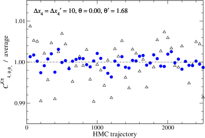
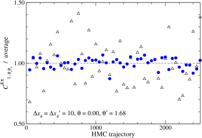
Figure 1: Statistical fluctuation of three-point function Cμ,ϕsϕsKπ(Δx4,Δx4;𝐩,𝐩)subscriptsuperscript𝐶𝐾𝜋𝜇subscriptitalic-ϕ𝑠subscriptitalic-ϕ𝑠Δsubscript𝑥4Δsuperscriptsubscript𝑥4𝐩superscript𝐩C^{K\pi}_{\mu,\phi_{s}\phi_{s}}({\Delta x_{4}},{\Delta x_{4}^{\prime}};{\bf p},{{\bf p}^{\prime}}) for μ=4𝜇4\mu\!=\!4 (left panel) and 1 (right panel). We plot the value for each jackknife sample normalized by the statistical average. The horizontal axis represents the HMC trajectory count of the excluded configuration in the jackknife analysis. The data are obtained at (ml,ms)=(0.015,0.080)subscript𝑚𝑙subscript𝑚𝑠0.0150.080(m_{l},m_{s})\!=\!(0.015,0.080) with Δx4=Δx4=10Δsubscript𝑥4Δsuperscriptsubscript𝑥410{\Delta x_{4}}\!=\!{\Delta x_{4}^{\prime}}\!=\!10, θ=0.00𝜃0.00\theta\!=\!0.00, θ=1.68superscript𝜃1.68\theta^{\prime}\!=\!1.68. Triangles and circles are data before and after averaging over the temporal location of the source operator x4subscript𝑥4x_{4}, respectively.

We estimate the remaining contribution from higher modes stochastically by using the noise method together with the dilution technique A2A:TrinLat . A complex Z2subscript𝑍2Z_{2} noise vector is prepared for each configuration, and is split into Nd=3×4×Nt/2subscript𝑁𝑑34subscript𝑁𝑡2N_{d}=3\times 4\times N_{t}/2 vectors ηd(x)(d=1,,Nd)subscript𝜂𝑑𝑥𝑑1subscript𝑁𝑑\eta_{d}(x)(d\!=\!1,\ldots,N_{d}). These diluted noise vectors have non-zero elements only for a single combination of color and spinor indices and at two consecutive time-slices. We solve a linear equation for each diluted noise vector

D(mq)xq=Phighηd(d=1,,Nd),𝐷subscript𝑚𝑞subscript𝑥𝑞subscript𝑃highsubscript𝜂𝑑𝑑1subscript𝑁𝑑\displaystyle D(m_{q})\,x_{q}=P_{\rm high}\,\eta_{d}\hskip 14.22636pt(d=1,\ldots,N_{d}),\hskip 5.69054pt (13)

where Phigh=1Plowsubscript𝑃high1subscript𝑃lowP_{\rm high}\!=\!1-P_{\rm low}, and Plow=k=1Neukuksubscript𝑃lowsuperscriptsubscript𝑘1subscript𝑁𝑒subscript𝑢𝑘superscriptsubscript𝑢𝑘P_{\rm low}\!=\!\sum_{k=1}^{N_{e}}u_{k}\,u_{k}^{\dagger} is the projector to the eigenspace spanned by the low-modes. The high-mode contribution is then estimated as

{D(mq)1}high(x,y)subscript𝐷superscriptsubscript𝑚𝑞1high𝑥𝑦\displaystyle\left\{D(m_{q})^{-1}\right\}_{\rm high}(x,y) =\displaystyle= d=1Ndxd(q)(x)ηd(y).superscriptsubscript𝑑1subscript𝑁𝑑superscriptsubscript𝑥𝑑𝑞𝑥superscriptsubscript𝜂𝑑𝑦\displaystyle\sum_{d=1}^{N_{d}}x_{d}^{(q)}(x)\,\eta_{d}^{\dagger}(y). (14)

We refer the readers to Refs. PFF:JLQCD:Nf2:RG+Ovr ; EMFF:JLQCD:Nf3:RG+Ovr for more details on our implementation.

Figure 1 shows the statistical fluctuation of the three-point function Cμ,ϕsϕsKπ(Δx4,Δx4;𝐩,𝐩)subscriptsuperscript𝐶𝐾𝜋𝜇subscriptitalic-ϕ𝑠subscriptitalic-ϕ𝑠Δsubscript𝑥4Δsuperscriptsubscript𝑥4𝐩superscript𝐩C^{K\pi}_{\mu,\phi_{s}\phi_{s}}({\Delta x_{4}},{\Delta x_{4}^{\prime}};{\bf p},{{\bf p}^{\prime}}) with a certain choice of Δx4()Δsuperscriptsubscript𝑥4{\Delta x_{4}}^{(\prime)} and 𝐩()superscript𝐩{\bf p}^{(\prime)}. Averaging over the temporal coordinate x4subscript𝑥4x_{4} reduces the statistical error by about a factor of 3 for the temporal component μ=4𝜇4\mu\!=\!4 and a factor of 5 for spatial μ=1𝜇1\mu\!=\!1.

The mssubscript𝑚𝑠m_{s} dependence of the form factors is studied by repeating our calculation at a different value of the strange quark mass ms=0.060superscriptsubscript𝑚𝑠0.060m_{s}^{\prime}\!=\!0.060 using the gauge ensemble at ms=0.040subscript𝑚𝑠0.040m_{s}\!=\!0.040 and the reweighing technique reweight:1 ; reweight:2 . For instance, the three-point function can be calculated as

Cμ,ϕϕPQmssubscriptdelimited-⟨⟩subscriptsuperscript𝐶𝑃𝑄𝜇italic-ϕsuperscriptitalic-ϕsuperscriptsubscript𝑚𝑠\displaystyle\langle C^{PQ}_{\mu,\,\phi\phi^{\prime}}\rangle_{m_{s}^{\prime}} =\displaystyle= Cμ,ϕϕPQw~(ms,ms)ms,subscriptdelimited-⟨⟩subscriptsuperscript𝐶𝑃𝑄𝜇italic-ϕsuperscriptitalic-ϕ~𝑤superscriptsubscript𝑚𝑠subscript𝑚𝑠subscript𝑚𝑠\displaystyle\langle C^{PQ}_{\mu,\,\phi\phi^{\prime}}\,\tilde{w}(m_{s}^{\prime},m_{s})\rangle_{m_{s}}, (15)

where ms()subscriptdelimited-⟨⟩superscriptsubscript𝑚𝑠\langle\cdots\rangle_{m_{s}^{(\prime)}} represents the Monte Carlo average at ms()superscriptsubscript𝑚𝑠m_{s}^{(\prime)}. The reweighting factor w~~𝑤\tilde{w} from mssubscript𝑚𝑠m_{s} to mssuperscriptsubscript𝑚𝑠m_{s}^{\prime} is defined as

w~(ms,ms)~𝑤superscriptsubscript𝑚𝑠subscript𝑚𝑠\displaystyle\tilde{w}(m_{s}^{\prime},m_{s}) =\displaystyle= w(ms,ms)w(ms,ms)ms,w(ms,ms)=det[D(ms)D(ms)]𝑤superscriptsubscript𝑚𝑠subscript𝑚𝑠subscriptdelimited-⟨⟩𝑤superscriptsubscript𝑚𝑠subscript𝑚𝑠subscript𝑚𝑠𝑤superscriptsubscript𝑚𝑠subscript𝑚𝑠delimited-[]𝐷superscriptsubscript𝑚𝑠𝐷subscript𝑚𝑠\displaystyle\frac{w(m_{s}^{\prime},m_{s})}{\langle w(m_{s}^{\prime},m_{s})\rangle_{m_{s}}},\hskip 14.22636ptw(m_{s}^{\prime},m_{s})=\det\left[\frac{D(m_{s}^{\prime})}{D(m_{s})}\right] (16)

for each gauge configuration. In order to remarkably reduce the computational cost, w𝑤w is decomposed into contributions from low- and high-modes

w(ms,ms)𝑤superscriptsubscript𝑚𝑠subscript𝑚𝑠\displaystyle w(m_{s}^{\prime},m_{s}) =\displaystyle= wlow(ms,ms)whigh(ms,ms),subscript𝑤lowsuperscriptsubscript𝑚𝑠subscript𝑚𝑠subscript𝑤highsuperscriptsubscript𝑚𝑠subscript𝑚𝑠\displaystyle w_{\rm low}(m_{s}^{\prime},m_{s})\,w_{\rm high}(m_{s}^{\prime},m_{s}), (17)
wlow(high)(ms,ms)subscript𝑤lowhighsuperscriptsubscript𝑚𝑠subscript𝑚𝑠\displaystyle w_{\rm low(high)}(m_{s}^{\prime},m_{s}) =\displaystyle= det[Plow(high)D(ms)D(ms)Plow(high)].delimited-[]subscript𝑃lowhigh𝐷superscriptsubscript𝑚𝑠𝐷subscript𝑚𝑠subscript𝑃lowhigh\displaystyle\det\left[P_{\rm low(high)}\frac{D(m_{s}^{\prime})}{D(m_{s})}P_{\rm low(high)}\right]. (18)

We exactly calculate the low mode contribution wlowsubscript𝑤loww_{\rm low} by using the low-lying eigenvalues, whereas the high-mode contribution whighsubscript𝑤highw_{\rm high} is estimated through a stochastic estimator for its square

whigh2(ms,ms)=1Nrr=1Nre12(Phighξr)(Ω1)Phighξr,superscriptsubscript𝑤high2superscriptsubscript𝑚𝑠subscript𝑚𝑠1subscript𝑁𝑟superscriptsubscript𝑟1subscript𝑁𝑟superscript𝑒12superscriptsubscript𝑃highsubscript𝜉𝑟Ω1subscript𝑃highsubscript𝜉𝑟\displaystyle w_{\rm{high}}^{2}(m_{s}^{\prime},m_{s})=\frac{1}{N_{r}}\sum_{r=1}^{N_{r}}e^{-\frac{1}{2}(P_{\rm high}\xi_{r})^{\dagger}(\Omega-1)P_{\rm high}\xi_{r}}, (19)

where ΩD(ms){D(ms)1}D(ms)1D(ms)Ω𝐷superscriptsubscript𝑚𝑠superscript𝐷superscriptsuperscriptsubscript𝑚𝑠1𝐷superscriptsuperscriptsubscript𝑚𝑠1𝐷subscript𝑚𝑠\Omega\equiv D(m_{s})^{\dagger}\{D(m_{s}^{\prime})^{-1}\}^{\dagger}D(m_{s}^{\prime})^{-1}D(m_{s}). In our study of the EM form factors EMFF:JLQCD:Nf3:RG+Ovr , the full reweighting factor ω𝜔\omega turned out to be largely dominated by the low-mode contribution wlowsubscript𝑤loww_{\rm low} with our simulation set-up. For each configuration, therefore, we use only ten Gaussian random vectors {ξ1,,ξ10}subscript𝜉1subscript𝜉10\{\xi_{1},...,\xi_{10}\} (Nr=10subscript𝑁𝑟10N_{r}\!=\!10) with which the uncertainty of w~~𝑤\tilde{w} due to the stochastic estimator is negligibly small compared to its statistical fluctuation.

III Form factors at simulation points

III.1 form factors
Refer to caption
Refer to caption
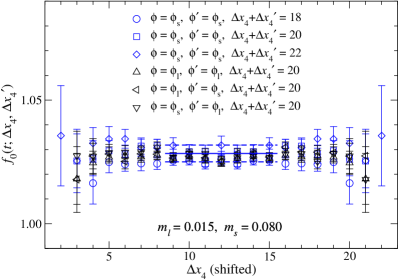
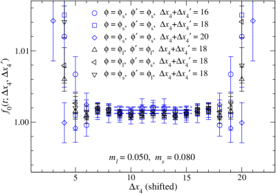
Figure 2: Effective value of f0(tmax)subscript𝑓0subscript𝑡maxf_{0}(t_{\rm max}) estimated from double ratio Rϕϕ(Δx4,Δx4)subscript𝑅italic-ϕsuperscriptitalic-ϕΔsubscript𝑥4Δsuperscriptsubscript𝑥4R_{\phi\phi^{\prime}}({\Delta x_{4}},{\Delta x_{4}^{\prime}}) at (ml,ms)=(0.050,0.080)subscript𝑚𝑙subscript𝑚𝑠0.0500.080(m_{l},m_{s})\!=\!(0.050,0.080) (left panel) and (0.015,0.080) (right panel). Blue circles, squares and diamond show data with the smeared source and sink for different values of Δx4+Δx4Δsubscript𝑥4Δsuperscriptsubscript𝑥4{\Delta x_{4}}+{\Delta x_{4}^{\prime}}. On the other hand, black triangles show data with local source and/or sink with Δx4+Δx4Δsubscript𝑥4Δsuperscriptsubscript𝑥4{\Delta x_{4}}+{\Delta x_{4}^{\prime}} kept fixed. All data are shifted along the horizontal axis so that the meson source and sink operators are located at T/4(Δx4+Δx4)/2𝑇4Δsubscript𝑥4Δsuperscriptsubscript𝑥42T/4-({\Delta x_{4}}+{\Delta x_{4}^{\prime}})/2 and T/4+(Δx4+Δx4)/2𝑇4Δsubscript𝑥4Δsuperscriptsubscript𝑥42T/4+({\Delta x_{4}}+{\Delta x_{4}^{\prime}})/2, respectively. Solid and dashed lines show a constant fit to data with different values of Δx4Δsubscript𝑥4{\Delta x_{4}} and Δx4+Δx4Δsubscript𝑥4Δsuperscriptsubscript𝑥4{\Delta x_{4}}+{\Delta x_{4}^{\prime}}.

In the limit of large temporal separations Δx4,Δx4Δsubscript𝑥4Δsuperscriptsubscript𝑥4{\Delta x_{4}},{\Delta x_{4}^{\prime}}\!\to\!\infty, the light meson three-point function (P,Q=π𝑃𝑄𝜋P,Q\!=\!\pi or K𝐾K) is dominated by the ground state contribution as

Cμ,ϕϕPQ(Δx4,Δx4;𝐩,𝐩)subscriptsuperscript𝐶𝑃𝑄𝜇italic-ϕsuperscriptitalic-ϕΔsubscript𝑥4Δsuperscriptsubscript𝑥4𝐩superscript𝐩\displaystyle C^{PQ}_{\mu,\phi\phi^{\prime}}({\Delta x_{4}},{\Delta x_{4}^{\prime}};{\bf p},{{\bf p}^{\prime}}) Δx4,Δx4Δsubscript𝑥4Δsuperscriptsubscript𝑥4absent\displaystyle\xrightarrow[{\Delta x_{4}},{\Delta x_{4}^{\prime}}\to\infty]{} ZQ,ϕ(𝐩)ZP,ϕ(𝐩)4EQ(𝐩)EP(𝐩)1ZVQ(p)|Vμ|P(p)subscript𝑍𝑄superscriptitalic-ϕsuperscriptsuperscript𝐩subscript𝑍𝑃italic-ϕ𝐩4subscript𝐸𝑄superscript𝐩subscript𝐸𝑃𝐩1subscript𝑍𝑉quantum-operator-product𝑄superscript𝑝subscript𝑉𝜇𝑃𝑝\displaystyle\frac{Z_{Q,\phi^{\prime}}({{\bf p}^{\prime}})^{*}\,Z_{P,\phi}({\bf p})}{4\,E_{Q}({{\bf p}^{\prime}})E_{P}({\bf p})}\frac{1}{Z_{V}}\langle Q(p^{\prime})|V_{\mu}|P(p)\rangle\, (20)
×eEQ(𝐩)Δx4eEP(𝐩)Δx4,absentsuperscript𝑒subscript𝐸𝑄superscript𝐩Δsuperscriptsubscript𝑥4superscript𝑒subscript𝐸𝑃𝐩Δsubscript𝑥4\displaystyle\hskip 71.13188pt\times e^{-E_{Q}({{\bf p}^{\prime}})\,{\Delta x_{4}^{\prime}}}e^{-E_{P}({\bf p})\,{\Delta x_{4}}},

where ZP,ϕ(𝐩)=P(p)|𝒪P,ϕsubscript𝑍𝑃italic-ϕ𝐩inner-product𝑃𝑝subscript𝒪𝑃italic-ϕZ_{P,\phi}({\bf p})\!=\!\langle P(p)|{{\mathcal{O}}}_{P,\phi}\rangle is the overlap of the meson interpolating field to the physical state, and ZVsubscript𝑍𝑉Z_{V} is the renormalization factor for the vector current. These factors and the exponential damping factors eEP(Q)(𝐩())Δx4()superscript𝑒subscript𝐸𝑃𝑄superscript𝐩Δsuperscriptsubscript𝑥4e^{-E_{P(Q)}({\bf p}^{(\prime)}){\Delta x_{4}}^{(\prime)}} cancel in the following double ratio dble_ratio ; Kl3:Rome:Nf0:Plq+Clv

Rϕϕ(Δx4,Δx4)subscript𝑅italic-ϕsuperscriptitalic-ϕΔsubscript𝑥4Δsuperscriptsubscript𝑥4\displaystyle R_{\phi\phi^{\prime}}({\Delta x_{4}},{\Delta x_{4}}^{\prime}) =\displaystyle= C4,ϕϕKπ(Δx4,Δx4;𝟎,𝟎)C4,ϕϕπK(Δx4,Δx4;𝟎,𝟎)C4,ϕϕKK(Δx4,Δx4;𝟎,𝟎)C4,ϕϕππ(Δx4,Δx4;𝟎,𝟎)subscriptsuperscript𝐶𝐾𝜋4italic-ϕsuperscriptitalic-ϕΔsubscript𝑥4Δsuperscriptsubscript𝑥400subscriptsuperscript𝐶𝜋𝐾4italic-ϕsuperscriptitalic-ϕΔsubscript𝑥4Δsuperscriptsubscript𝑥400subscriptsuperscript𝐶𝐾𝐾4italic-ϕsuperscriptitalic-ϕΔsubscript𝑥4Δsuperscriptsubscript𝑥400subscriptsuperscript𝐶𝜋𝜋4italic-ϕsuperscriptitalic-ϕΔsubscript𝑥4Δsuperscriptsubscript𝑥400\displaystyle\frac{C^{K\pi}_{4,\phi\phi^{\prime}}({\Delta x_{4}},{\Delta x_{4}^{\prime}};{\bf 0},{\bf 0})C^{\pi K}_{4,\phi\phi^{\prime}}({\Delta x_{4}},{\Delta x_{4}^{\prime}};{\bf 0},{\bf 0})}{C^{KK}_{4,\phi\phi^{\prime}}({\Delta x_{4}},{\Delta x_{4}^{\prime}};{\bf 0},{\bf 0})C^{\pi\pi}_{4,\phi\phi^{\prime}}({\Delta x_{4}},{\Delta x_{4}^{\prime}};{\bf 0},{\bf 0})} (21)
Δx4,Δx4(MK+Mπ)24MKMπf0(tmax)2,Δsubscript𝑥4Δsuperscriptsubscript𝑥4absentabsentsuperscriptsubscript𝑀𝐾subscript𝑀𝜋24subscript𝑀𝐾subscript𝑀𝜋subscript𝑓0superscriptsubscript𝑡max2\displaystyle\xrightarrow[{\Delta x_{4}},{\Delta x_{4}^{\prime}}\to\infty]{}\frac{(M_{K}+M_{\pi})^{2}}{4M_{K}M_{\pi}}f_{0}(t_{\rm max})^{2},

from which we calculate the scalar form factor f0(tmax)subscript𝑓0subscript𝑡maxf_{0}(t_{\rm max}) at the largest momentum transfer tmaxsubscript𝑡maxt_{\rm max}. Figure 2 shows the effective value of f0(tmax)subscript𝑓0subscript𝑡maxf_{0}(t_{\rm max}) as a function of Δx4Δsubscript𝑥4{\Delta x_{4}}. The accuracy of f0(tmax)subscript𝑓0subscript𝑡maxf_{0}(t_{\rm max}) is typically 1less-than-or-similar-toabsent1\lesssim\!1 % with our simulation set-up. The figure also demonstrates that the all-to-all quark propagator greatly helps us increase the reliability of the precision calculation of f0(tmax)subscript𝑓0subscript𝑡maxf_{0}(t_{\rm max}): it enables us to confirm the consistency in f0(tmax)subscript𝑓0subscript𝑡maxf_{0}(t_{\rm max}) among different values of Δx4+Δx4Δsubscript𝑥4Δsuperscriptsubscript𝑥4{\Delta x_{4}}+{\Delta x_{4}^{\prime}} and different smearing functions for the meson interpolating fields.

At smaller momentum transfer t<tmax𝑡subscript𝑡maxt<t_{\rm max}, the vector form factor f+(t)subscript𝑓𝑡f_{+}(t) and the ratio ξ(t)=f(t)/f+(t)𝜉𝑡subscript𝑓𝑡subscript𝑓𝑡\xi(t)=f_{-}(t)/f_{+}(t) are calculated from the following ratios Kl3:Rome:Nf0:Plq+Clv ; Kl3:JLQCD:Nf2:Plq+Clv ; Kl3:RBC:Nf2:DBW2+DWF

R~ϕϕ(𝐩,𝐩;Δx4,Δx4)=C4,ϕϕKπ(Δx4,Δx4;𝐩,𝐩)CϕϕlK(Δx4,𝟎)Cϕlϕπ(Δx4,𝟎)C4,ϕϕKπ(Δx4,Δx4;𝟎,𝟎)CϕϕlK(Δx4,𝐩)Cϕlϕπ(Δx4,𝐩)subscript~𝑅italic-ϕsuperscriptitalic-ϕ𝐩superscript𝐩Δsubscript𝑥4Δsuperscriptsubscript𝑥4subscriptsuperscript𝐶𝐾𝜋4italic-ϕsuperscriptitalic-ϕΔsubscript𝑥4Δsuperscriptsubscript𝑥4𝐩superscript𝐩subscriptsuperscript𝐶𝐾italic-ϕsubscriptitalic-ϕ𝑙Δsubscript𝑥40subscriptsuperscript𝐶𝜋subscriptitalic-ϕ𝑙superscriptitalic-ϕΔsuperscriptsubscript𝑥40subscriptsuperscript𝐶𝐾𝜋4italic-ϕsuperscriptitalic-ϕΔsubscript𝑥4Δsuperscriptsubscript𝑥400subscriptsuperscript𝐶𝐾italic-ϕsubscriptitalic-ϕ𝑙Δsubscript𝑥4𝐩subscriptsuperscript𝐶𝜋subscriptitalic-ϕ𝑙superscriptitalic-ϕΔsuperscriptsubscript𝑥4superscript𝐩\displaystyle\tilde{R}_{\phi\phi^{\prime}}({\bf p},{{\bf p}^{\prime}};{\Delta x_{4}},{\Delta x_{4}^{\prime}})=\frac{C^{K\pi}_{4,\phi\phi^{\prime}}({\Delta x_{4}},{\Delta x_{4}^{\prime}};{\bf p},{{\bf p}^{\prime}})C^{K}_{\phi\phi_{l}}({\Delta x_{4}},{\bf 0})\,C^{\pi}_{\phi_{l}\phi^{\prime}}({\Delta x_{4}^{\prime}},{\bf 0})}{C^{K\pi}_{4,\phi\phi^{\prime}}({\Delta x_{4}},{\Delta x_{4}^{\prime}};{\bf 0},{\bf 0})C^{K}_{\phi\phi_{l}}({\Delta x_{4}},{\bf p})\,C^{\pi}_{\phi_{l}\phi^{\prime}}({\Delta x_{4}^{\prime}},{{\bf p}^{\prime}})}
Δx4,Δx4{EK(𝐩)+Eπ(𝐩)MK+Mπ+EK(𝐩)Eπ(𝐩)MK+Mπξ(t)}f+(t)f0(tmax),Δsubscript𝑥4Δsuperscriptsubscript𝑥4absentabsentsubscript𝐸𝐾𝐩subscript𝐸𝜋superscript𝐩subscript𝑀𝐾subscript𝑀𝜋subscript𝐸𝐾𝐩subscript𝐸𝜋superscript𝐩subscript𝑀𝐾subscript𝑀𝜋𝜉𝑡subscript𝑓𝑡subscript𝑓0subscript𝑡max\displaystyle\xrightarrow[{\Delta x_{4}},{\Delta x_{4}^{\prime}}\to\infty]{}\left\{\frac{E_{K}({\bf p})+E_{\pi}({{\bf p}^{\prime}})}{M_{K}+M_{\pi}}+\frac{E_{K}({\bf p})-E_{\pi}({{\bf p}^{\prime}})}{M_{K}+M_{\pi}}\xi(t)\right\}\frac{f_{+}(t)}{f_{0}(t_{\rm max})},\hskip 25.60747pt (22)
Rk,ϕϕ(𝐩,𝐩;Δx4,Δx4)=Ck,ϕϕKπ(Δx4,Δx4;𝐩,𝐩)C4,ϕϕKK(Δx4,Δx4;𝐩,𝐩)C4,ϕϕKπ(Δx4,Δx4;𝐩,𝐩)Ck,ϕϕKK(Δx4,Δx4;𝐩,𝐩)subscript𝑅𝑘italic-ϕsuperscriptitalic-ϕ𝐩superscript𝐩Δsubscript𝑥4Δsuperscriptsubscript𝑥4subscriptsuperscript𝐶𝐾𝜋𝑘italic-ϕsuperscriptitalic-ϕΔsubscript𝑥4Δsuperscriptsubscript𝑥4𝐩superscript𝐩subscriptsuperscript𝐶𝐾𝐾4italic-ϕsuperscriptitalic-ϕΔsubscript𝑥4Δsuperscriptsubscript𝑥4𝐩superscript𝐩subscriptsuperscript𝐶𝐾𝜋4italic-ϕsuperscriptitalic-ϕΔsubscript𝑥4Δsuperscriptsubscript𝑥4𝐩superscript𝐩subscriptsuperscript𝐶𝐾𝐾𝑘italic-ϕsuperscriptitalic-ϕΔsubscript𝑥4Δsuperscriptsubscript𝑥4𝐩superscript𝐩\displaystyle R_{k,\phi\phi^{\prime}}({\bf p},{{\bf p}^{\prime}};{\Delta x_{4}},{\Delta x_{4}^{\prime}})=\frac{C^{K\pi}_{k,\phi\phi^{\prime}}({\Delta x_{4}},{\Delta x_{4}^{\prime}};{\bf p},{{\bf p}^{\prime}})C^{KK}_{4,\phi\phi^{\prime}}({\Delta x_{4}},{\Delta x_{4}^{\prime}};{\bf p},{{\bf p}^{\prime}})}{C^{K\pi}_{4,\phi\phi^{\prime}}({\Delta x_{4}},{\Delta x_{4}^{\prime}};{\bf p},{{\bf p}^{\prime}})C^{KK}_{k,\phi\phi^{\prime}}({\Delta x_{4}},{\Delta x_{4}^{\prime}};{\bf p},{{\bf p}^{\prime}})}
Δx4,Δx4EK(𝐩)+EK(𝐩)(p+p)k(p+p)k+(pp)kξ(t)EK(𝐩)+Eπ(𝐩)+{EK(𝐩)Eπ(𝐩)}ξ(t).Δsubscript𝑥4Δsuperscriptsubscript𝑥4absentabsentsubscript𝐸𝐾𝐩subscript𝐸𝐾superscript𝐩subscript𝑝superscript𝑝𝑘subscript𝑝superscript𝑝𝑘subscript𝑝superscript𝑝𝑘𝜉𝑡subscript𝐸𝐾𝐩subscript𝐸𝜋superscript𝐩subscript𝐸𝐾𝐩subscript𝐸𝜋superscript𝐩𝜉𝑡\displaystyle\hskip 14.22636pt\xrightarrow[{\Delta x_{4}},{\Delta x_{4}^{\prime}}\to\infty]{}\frac{E_{K}({\bf p})+E_{K}({{\bf p}^{\prime}})}{(p+{p^{\prime}})_{k}}\frac{(p+{p^{\prime}})_{k}+(p-{p^{\prime}})_{k}\xi(t)}{E_{K}({\bf p})+E_{\pi}({{\bf p}^{\prime}})+\left\{E_{K}({\bf p})-E_{\pi}({{\bf p}^{\prime}})\right\}\xi(t)}. (23)

The last line of Eq. (22) assumes the asymptotic form of the two-point function

CϕϕP(Δx4;𝐩)subscriptsuperscript𝐶𝑃italic-ϕsuperscriptitalic-ϕΔsubscript𝑥4𝐩\displaystyle C^{P}_{\phi\phi^{\prime}}({\Delta x_{4}};{\bf p}) Δx4Δsubscript𝑥4absent\displaystyle\xrightarrow[{\Delta x_{4}}\to\infty]{} ZP,ϕ(𝐩)ZP,ϕ(𝐩)2EP(𝐩)eEP(𝐩)Δx4.subscript𝑍𝑃superscriptitalic-ϕsuperscript𝐩subscript𝑍𝑃italic-ϕ𝐩2subscript𝐸𝑃𝐩superscript𝑒subscript𝐸𝑃𝐩Δsubscript𝑥4\displaystyle\frac{Z_{P,\phi^{\prime}}({\bf p})^{*}\,Z_{P,\phi}({\bf p})}{2\,E_{P}({\bf p})}\,e^{-E_{P}({\bf p})\,{\Delta x_{4}}}. (24)

We evaluate f0(t)subscript𝑓0𝑡f_{0}(t) from f+(t)subscript𝑓𝑡f_{+}(t) and ξ(t)𝜉𝑡\xi(t) at t<tmax𝑡subscript𝑡maxt<t_{\rm max}. Note that, at tmaxsubscript𝑡maxt_{\rm max}, we only have results for f0(tmax)subscript𝑓0subscript𝑡maxf_{0}(t_{\rm max}) from Rϕϕsubscript𝑅italic-ϕsuperscriptitalic-ϕR_{\phi\phi^{\prime}}, since R~ϕϕsubscript~𝑅italic-ϕsuperscriptitalic-ϕ\tilde{R}_{\phi\phi^{\prime}} and Rk,ϕϕsubscript𝑅𝑘italic-ϕsuperscriptitalic-ϕR_{k,\phi\phi^{\prime}} have no sensitivity to f+subscript𝑓f_{+} and ξ𝜉\xi.

Refer to caption
Refer to caption
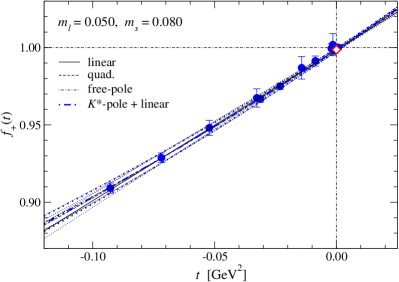
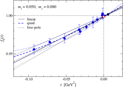
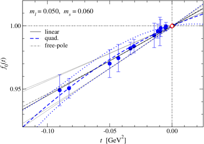
Figure 3: Vector (left panel) and scalar form factors (right panel) as a function of t𝑡t at (ml,ms)=(0.050,0.080)subscript𝑚𝑙subscript𝑚𝑠0.0500.080(m_{l},m_{s})\!=\!(0.050,0.080). Solid circles show the results at simulated t𝑡t’s. Solid, dashed and dot-dashed lines are linear, quadratic (26) and free-pole fits (27), respectively. We also plot the fit with the Ksuperscript𝐾K^{*} pole (25) for f+subscript𝑓f_{+}. The dotted lines show their statistical error. The value interpolated to t=0𝑡0t\!=\!0 is shown by the open diamond. The blue thicker lines show the fit to estimate the central value and statistical error of the interpolated value.
Refer to caption
Refer to caption
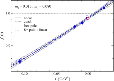
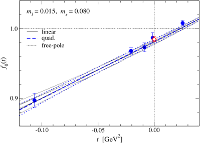
Figure 4: Same as Fig. 3, but for (ml,ms)=(0.015,0.080)subscript𝑚𝑙subscript𝑚𝑠0.0150.080(m_{l},m_{s})\!=\!(0.015,0.080).
Refer to caption
Refer to caption
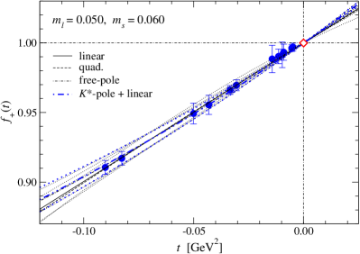
Figure 5: Same as Fig. 3, but for (ml,ms)=(0.050,0.060)subscript𝑚𝑙subscript𝑚𝑠0.0500.060(m_{l},m_{s})\!=\!(0.050,0.060).

In Figs. 3 and 4, we plot the vector and scalar form factors as a function of t𝑡t. At ms=0.080subscript𝑚𝑠0.080m_{s}\!=\!0.080, the statistical accuracy of the non-trivial chiral correction f{+,0}(t)1subscript𝑓0𝑡1f_{\{+,0\}}(t)-1 due to msmlsubscript𝑚𝑠subscript𝑚𝑙m_{s}\!\neq\!m_{l} and t0𝑡0t\!\neq\!0 is typically 10 – 20 %. Analyses based on ChPT suggest that finite volume effects including those due to the twisted boundary condition FVE:ChPT:TBC:BR are below this accuracy: O(exp[MπL])O(2%)less-than-or-similar-to𝑂subscript𝑀𝜋𝐿𝑂percent2O(\exp[-M_{\pi}L])\!\lesssim\!O(2\,\%) or less FVE:ChPT:TBC:GS ; FVE:ChPT:TBC:BR ; FVE:ChPT:TBC:BBGR .

In Fig. 5, we observe that the statistical error is about a factor of two larger at ms=0.060subscript𝑚𝑠0.060m_{s}\!=\!0.060 due to reweighting.

We parametrize the t𝑡t dependence of the form factors f{+,0}subscript𝑓0f_{\{+,0\}} to estimate the normalization f+(0)=f0(0)subscript𝑓0subscript𝑓00f_{+}(0)\!=\!f_{0}(0) and the slopes df{+,0}/dt|t=0evaluated-at𝑑subscript𝑓0𝑑𝑡𝑡0df_{\{+,0\}}/dt|_{t=0} at simulated quark masses. For the vector form factor f+subscript𝑓f_{+}, we use the following parametrization based on the vector meson dominance (VMD) hypothesis

f+(t)subscript𝑓𝑡\displaystyle f_{+}(t) =\displaystyle= f+(0){11t/MK2+at},subscript𝑓011𝑡superscriptsubscript𝑀superscript𝐾2𝑎𝑡\displaystyle f_{+}(0)\left\{\frac{1}{1-t/M_{K^{*}}^{2}}+at\right\}, (25)

where MKsubscript𝑀superscript𝐾M_{K^{*}} represents the strange-light vector meson mass calculated at simulation points. There could be contribution of the higher poles and cuts, which is well approximated by the additional linear term at our small values of |t|𝑡|t|. We note that our data of the pion and kaon EM form factors in a similar region of t𝑡t are well described by this type of the parametrization EMFF:JLQCD:Nf3:RG+Ovr .

Since we simulate small values of |t|𝑡|t|, our data of f{+,0}subscript𝑓0f_{\{+,0\}} does not show any strong curvature in Figs. 3 – 5, and simple polynomial parametrization also describes our data well

f{+,0}(t)subscript𝑓0𝑡\displaystyle f_{\{+,0\}}(t) =\displaystyle= f+(0){1+λ{+,0}tMπ±,phys2+λ{+,0}′′(tMπ±,phys2)2}subscript𝑓01superscriptsubscript𝜆0𝑡superscriptsubscript𝑀superscript𝜋plus-or-minusphys2superscriptsubscript𝜆0′′superscript𝑡superscriptsubscript𝑀superscript𝜋plus-or-minusphys22\displaystyle f_{+}(0)\left\{1+\lambda_{\{+,0\}}^{\prime}\,\frac{t}{M_{\pi^{\pm},\rm phys}^{2}}+\lambda_{\{+,0\}}^{\prime\prime}\left(\frac{t}{M_{\pi^{\pm},\rm phys}^{2}}\right)^{2}\right\} (26)

even without the quadratic term. The conventional free-pole form

f{+,0}(t)subscript𝑓0𝑡\displaystyle f_{\{+,0\}}(t) =\displaystyle= f{+,0}(0)1t/Mpole,{+,0}2subscript𝑓001𝑡superscriptsubscript𝑀pole02\displaystyle\frac{f_{\{+,0\}}(0)}{1-t/M_{{\rm pole},\{+,0\}}^{2}} (27)

also works well.

Table 2: Fit results for normalization f+(0)subscript𝑓0f_{+}(0) and slope parameters λ{+,0}superscriptsubscript𝜆0\lambda_{\{+,0\}}^{\prime}.
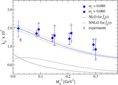
mlsubscript𝑚𝑙m_{l} mssubscript𝑚𝑠m_{s} f+(0)subscript𝑓0f_{+}(0) λ+×102superscriptsubscript𝜆superscript102\lambda_{+}^{\prime}\!\times\!10^{2} λ0×102superscriptsubscript𝜆0superscript102\lambda_{0}^{\prime}\!\times\!10^{2}
0.050 0.080 0.9986(11)()1+20.9986(11)\left({}^{+2}_{-1}\right) 2.02(7)(12)2.027122.02(7)(12) 1.10(28)(11)1.1028111.10(28)(11)
0.050 0.060 0.99991(25)(8)0.999912580.99991(25)(-8) 2.12(14)(22)2.1214222.12(14)(22) 0.84(51)(27)0.8451270.84(51)(27)
0.035 0.080 0.9937(31)(+8)0.99373180.9937(31)(+8) 2.37(11)(18)2.3711182.37(11)(18) 1.42(29)(11)1.4229111.42(29)(11)
0.035 0.060 0.9977(20)()2+40.9977(20)\left({}^{+4}_{-2}\right) 2.52(19)(19)2.5219192.52(19)(19) 1.72(42)(26)1.7242261.72(42)(26)
0.025 0.080 0.9919(18)()5+70.9919(18)\left({}^{+7}_{-5}\right) 2.51(5)(21)2.515212.51(5)(21) 1.46(17)(7)1.461771.46(17)(7)
0.025 0.060 0.9969(46)()11+10.9969(46)\left({}^{+1}_{-11}\right) 2.74(14)(26)2.7414262.74(14)(26) 1.59(52)(18)1.5952181.59(52)(18)
0.015 0.080 0.9847(34)()5+40.9847(34)\left({}^{+4}_{-5}\right) 2.72(10)(22)2.7210222.72(10)(22) 1.70(15)(1)1.701511.70(15)(1)
0.015 0.060 0.9922(74)()7+180.9922(74)\left({}^{+18}_{-7}\right) 2.75(13)(32)2.7513322.75(13)(32) 1.92(32)(14)1.9232141.92(32)(14)

In this study, we estimate f+(0)subscript𝑓0f_{+}(0) and df{+,0}/dt|t=0evaluated-at𝑑subscript𝑓0𝑑𝑡𝑡0df_{\{+,0\}}/dt|_{t=0} by a simultaneous fit using the VMD-based form (25) for f+subscript𝑓f_{+} and the quadratic form (26) for f0subscript𝑓0f_{0}. The uncertainty due to the choice of the fitting form is estimated by testing the polynomial and free-pole forms for f+subscript𝑓f_{+} and the linear and free-pole forms for f0subscript𝑓0f_{0}. Fit results are summarized in Table 2, where we list the phenomenologically familiar slope parameter λ{+,0}superscriptsubscript𝜆0\lambda_{\{+,0\}}^{\prime} in the quadratic parametrization (26) instead of df{+,0}/dt|t=0=f+(0)λ{+,0}/Mπ±,phys2evaluated-at𝑑subscript𝑓0𝑑𝑡𝑡0subscript𝑓0superscriptsubscript𝜆0superscriptsubscript𝑀superscript𝜋plus-or-minusphys2df_{\{+,0\}}/dt|_{t=0}\!=\!f_{+}(0)\lambda_{\{+,0\}}^{\prime}/M_{\pi^{\pm},\rm phys}^{2}.

In the simulated region of t𝑡t, all the aforementioned parametrizations describe our data well with χ2/d.o.f0.5formulae-sequencesuperscript𝜒2doless-than-or-similar-tof0.5\chi^{2}/{\rm d.o.f}\!\lesssim\!0.5. The choice of the parametrization leads to small uncertainty for f+(0)subscript𝑓0f_{+}(0) compared to the statistical accuracy. For the slope parameter λ{+,0}superscriptsubscript𝜆0\lambda_{\{+,0\}}^{\prime}, the systematic error is more important, but not so large compared to the statistical one.

IV Chiral extrapolation of form factors

IV.1 ChPT formulae and LECs

The momentum transfer and quark mass dependence of the form factors is known up to NNLO in SU(3) ChPT KFF:weak:ChPT:SU3:NNLO:PS ; KFF:weak:ChPT:SU3:NNLO:BT . Let us denote the chiral expansion as

fX(t)subscript𝑓𝑋𝑡\displaystyle f_{X}(t) =\displaystyle= fX,0+fX,2(t)+fX,4(t)+fX,6(t)(X=+,,0),subscript𝑓𝑋0subscript𝑓𝑋2𝑡subscript𝑓𝑋4𝑡subscript𝑓𝑋6𝑡𝑋0\displaystyle f_{X,0}+f_{X,2}(t)+f_{X,4}(t)+f_{X,6}(t)\hskip 8.53581pt(X=+,-,0), (28)

where fX,0subscript𝑓𝑋0f_{X,0}, fX,2subscript𝑓𝑋2f_{X,2}, and fX,4subscript𝑓𝑋4f_{X,4}, represent the LO, NLO, and NNLO contributions, respectively. We add a possible higher order term fX,6subscript𝑓𝑋6f_{X,6}, the functional form of which is not yet known.

The current conservation fixes the normalization of the vector form factor in the chiral limit as f+,0=1subscript𝑓01f_{+,0}\!=\!1. The NLO contribution can be decomposed into two parts

f+,2(t)subscript𝑓2𝑡\displaystyle f_{+,2}(t) =\displaystyle= f+,2,L(t)+f+,2,B(t).subscript𝑓2𝐿𝑡subscript𝑓2𝐵𝑡\displaystyle f_{+,2,L}(t)+f_{+,2,B}(t). (29)

The first part f+,2,Lsubscript𝑓2𝐿f_{+,2,L} represents the analytic term arising from the tree diagram with a vertex arising from the O(p4)𝑂superscript𝑝4O(p^{4}) chiral Lagrangian 4subscript4{\mathcal{L}}_{4},

Fπ2f+,2,L(t)superscriptsubscript𝐹𝜋2subscript𝑓2𝐿𝑡\displaystyle F_{\pi}^{2}\,f_{+,2,L}(t) =\displaystyle= 2L9rt.2superscriptsubscript𝐿9𝑟𝑡\displaystyle 2L_{9}^{r}t. (30)

Note that p𝑝p symbolically represents the Nambu-Goldstone (NG) boson momentum, and L9rsuperscriptsubscript𝐿9𝑟L_{9}^{r} is a LEC in 4subscript4{\mathcal{L}}_{4}. This contribution does not involve quark masses to be compatible with the current conservation f+,2,L(0)=0subscript𝑓2𝐿00f_{+,2,L}(0)\!=\!0.

The other part is the contribution of loop diagrams

Fπ2f+,2,B(t)superscriptsubscript𝐹𝜋2subscript𝑓2𝐵𝑡\displaystyle F_{\pi}^{2}\,f_{+,2,B}(t) =\displaystyle= 38{A¯(Mπ2)+2A¯(MK2)+A¯(Mη2)}38¯𝐴superscriptsubscript𝑀𝜋22¯𝐴superscriptsubscript𝑀𝐾2¯𝐴superscriptsubscript𝑀𝜂2\displaystyle\frac{3}{8}\left\{\bar{A}(M_{\pi}^{2})+2\bar{A}(M_{K}^{2})+\bar{A}(M_{\eta}^{2})\right\} (31)
32{B¯22(Mπ2,MK2,t)+B¯22(MK2,Mη2,t)},32subscript¯𝐵22superscriptsubscript𝑀𝜋2superscriptsubscript𝑀𝐾2𝑡subscript¯𝐵22superscriptsubscript𝑀𝐾2superscriptsubscript𝑀𝜂2𝑡\displaystyle\hskip 28.45274pt-\frac{3}{2}\left\{\bar{B}_{22}(M_{\pi}^{2},M_{K}^{2},t)+\bar{B}_{22}(M_{K}^{2},M_{\eta}^{2},t)\right\},

where A¯¯𝐴\bar{A} and B¯22subscript¯𝐵22\bar{B}_{22} represent one-loop integral functions. We refer the readers to Refs. EMFF:JLQCD:Nf3:RG+Ovr ; PFF+KFF:ChPT:NNLO:Nf3 for their definition and expression. Note that the so-called ξ𝜉\xi-expansion is employed in this study: the form factors are expanded in terms of ξ{π,K,η}=M{π,K,η}2/(4πFπ)2subscript𝜉𝜋𝐾𝜂superscriptsubscript𝑀𝜋𝐾𝜂2superscript4𝜋subscript𝐹𝜋2\xi_{\{\pi,K,\eta\}}\!=\!M_{\{\pi,K,\eta\}}^{2}/(4\pi F_{\pi})^{2}, where Fπsubscript𝐹𝜋F_{\pi} represents the pion decay constant. In Ref. Spectrum:Nf2:RG+Ovr:JLQCD , we demonstrated that the ξ𝜉\xi-expansion of the meson masses and decay constants has a better convergence than the expansion in terms of mq/(4πF0)2subscript𝑚𝑞superscript4𝜋subscript𝐹02m_{q}/(4\pi F_{0})^{2}. Here F0subscript𝐹0F_{0} is the decay constant in the chiral limit. The ξ𝜉\xi-expansion has another important advantage that ChPT formulae are free from the unknown LEC F0subscript𝐹0F_{0}.

This is also the case for the NNLO contribution

f+,4(t)subscript𝑓4𝑡\displaystyle f_{+,4}(t) =\displaystyle= f+,4,C(t)+f+,4,L(t)+f+,4,B(t).subscript𝑓4𝐶𝑡subscript𝑓4𝐿𝑡subscript𝑓4𝐵𝑡\displaystyle f_{+,4,C}(t)+f_{+,4,L}(t)+f_{+,4,B}(t). (32)

Here f+,4,Bsubscript𝑓4𝐵f_{+,4,B} represents the contribution of two-loop diagrams without any vertices from 4subscript4{\mathcal{L}}_{4} and O(p6)𝑂superscript𝑝6O(p^{6}) chiral Lagrangians 6subscript6{\mathcal{L}}_{6} ChPT:SU3:NNLO . While its expression is rather lengthy KFF:weak:ChPT:SU3:NNLO:BT:loop , it does not contain any LECs in the ξ𝜉\xi - expansion, and is not an obstacle to obtaining a stable chiral extrapolation.

The term f+,4,Lsubscript𝑓4𝐿f_{+,4,L} mainly arises from the one-loop diagrams with one vertex from 4subscript4\mathcal{L}_{4}, and hence depends on the O(p4)𝑂superscript𝑝4O(p^{4}) couplings Lirsuperscriptsubscript𝐿𝑖𝑟L_{i}^{r}. At the level of NLO, only L9rsuperscriptsubscript𝐿9𝑟L_{9}^{r} appears in f+,2,Lsubscript𝑓2𝐿f_{+,2,L}, and we fix it to an estimate obtained from our study of the EM form factors EMFF:JLQCD:Nf3:RG+Ovr . Other L{1 8}subscript𝐿18L_{\{1\,-\,8\}} appear only in small NNLO term f+,4,Lsubscript𝑓4𝐿f_{+,4,L}. We fix them to a recent phenomenological estimate in Ref. ChPT:LECs:SU2+SU3 . These input values are listed in Table 3.

Table 3: Input values for O(p4)𝑂superscript𝑝4O(p^{4}) couplings Lirsuperscriptsubscript𝐿𝑖𝑟L_{i}^{r} at renormalization scale μ=Mρ𝜇subscript𝑀𝜌\mu\!=\!M_{\rho}. We use L9rsuperscriptsubscript𝐿9𝑟L_{9}^{r} from our study of the EM form factors EMFF:JLQCD:Nf3:RG+Ovr , whereas L{1 8}subscript𝐿18L_{\{1\,-\,8\}} are taken from a phenomenological study ChPT:LECs:SU2+SU3 . In that paper, authors presented two estimates obtained from different ChPT fits of experimental data. The central value and the first statistical error of L{1 8}subscript𝐿18L_{\{1\,-\,8\}} are from the authors’ preferred fit, whereas we assign the difference between the two estimates as the second systematic error.
L1r×103superscriptsubscript𝐿1𝑟superscript103L_{1}^{r}\!\times\!10^{3} L2r×103superscriptsubscript𝐿2𝑟superscript103L_{2}^{r}\!\times\!10^{3} L3r×103superscriptsubscript𝐿3𝑟superscript103L_{3}^{r}\!\times\!10^{3} L4r×103superscriptsubscript𝐿4𝑟superscript103L_{4}^{r}\!\times\!10^{3} L5r×103superscriptsubscript𝐿5𝑟superscript103L_{5}^{r}\!\times\!10^{3}
0.53(6)(+11) 0.81(4)(-22) -3.07(20)(+27) 0.3(0)(+0.46) 1.01(6)(-51)
L6r×103superscriptsubscript𝐿6𝑟superscript103L_{6}^{r}\!\times\!10^{3} L7r×103superscriptsubscript𝐿7𝑟superscript103L_{7}^{r}\!\times\!10^{3} L8r×103superscriptsubscript𝐿8𝑟superscript103L_{8}^{r}\!\times\!10^{3} L9r×103superscriptsubscript𝐿9𝑟superscript103L_{9}^{r}\!\times\!10^{3}
0.14(5)(+35) -0.34(9)(+15) 0.47(10)(-30) 4.6(1.1)()0.5+0.14.6(1.1)\left({}^{+0.1}_{-0.5}\right)

The NNLO analytic term f+,4,Csubscript𝑓4𝐶f_{+,4,C} arises from tree-diagrams with one vertex from 6subscript6\mathcal{L}_{6}. A central issue in our analysis based on NNLO ChPT is how to deal with many O(p6)𝑂superscript𝑝6O(p^{6}) couplings Cirsuperscriptsubscript𝐶𝑖𝑟C_{i}^{r} appearing in this contribution

Fπ4f+,4,Csuperscriptsubscript𝐹𝜋4subscript𝑓4𝐶\displaystyle F_{\pi}^{4}f_{+,4,C} =\displaystyle= 8c+,πKr(MK2Mπ2)24c+,πtrMπ2t4c+,KtrMK2t4ct2rt2,8superscriptsubscript𝑐𝜋𝐾𝑟superscriptsuperscriptsubscript𝑀𝐾2superscriptsubscript𝑀𝜋224superscriptsubscript𝑐𝜋𝑡𝑟superscriptsubscript𝑀𝜋2𝑡4superscriptsubscript𝑐𝐾𝑡𝑟superscriptsubscript𝑀𝐾2𝑡4superscriptsubscript𝑐superscript𝑡2𝑟superscript𝑡2\displaystyle-8{c_{+,\pi K}^{r}}\,(M_{K}^{2}-M_{\pi}^{2})^{2}-4{c_{+,\pi t}^{r}}\,M_{\pi}^{2}\,t-4{c_{+,Kt}^{r}}\,M_{K}^{2}\,t-4{c_{t^{2}}^{r}}\,t^{2}, (33)

where the coefficients cXrsubscriptsuperscript𝑐𝑟𝑋c^{r}_{X}’s are linear combinations of O(p6)𝑂superscript𝑝6O(p^{6}) couplings

c+,πKrsuperscriptsubscript𝑐𝜋𝐾𝑟\displaystyle{c_{+,\pi K}^{r}} =\displaystyle= C12r+C34r,superscriptsubscript𝐶12𝑟superscriptsubscript𝐶34𝑟\displaystyle C_{12}^{r}+C_{34}^{r}, (34)
c+,πtrsuperscriptsubscript𝑐𝜋𝑡𝑟\displaystyle c_{+,\pi t}^{r} =\displaystyle= 2C12r+4C13r+C64r+C65r+C90r,2superscriptsubscript𝐶12𝑟4superscriptsubscript𝐶13𝑟superscriptsubscript𝐶64𝑟superscriptsubscript𝐶65𝑟superscriptsubscript𝐶90𝑟\displaystyle 2C_{12}^{r}+4C_{13}^{r}+C_{64}^{r}+C_{65}^{r}+C_{90}^{r}, (35)
c+,Ktrsuperscriptsubscript𝑐𝐾𝑡𝑟\displaystyle c_{+,Kt}^{r} =\displaystyle= 2C12r+8C13r+2C63r+2C64r+C90r,2superscriptsubscript𝐶12𝑟8superscriptsubscript𝐶13𝑟2superscriptsubscript𝐶63𝑟2superscriptsubscript𝐶64𝑟superscriptsubscript𝐶90𝑟\displaystyle 2C_{12}^{r}+8C_{13}^{r}+2C_{63}^{r}+2C_{64}^{r}+C_{90}^{r}, (36)
ct2rsuperscriptsubscript𝑐superscript𝑡2𝑟\displaystyle{c_{t^{2}}^{r}} =\displaystyle= C88rC90r.superscriptsubscript𝐶88𝑟superscriptsubscript𝐶90𝑟\displaystyle C_{88}^{r}-C_{90}^{r}. (37)

Similar to the case of Lirsuperscriptsubscript𝐿𝑖𝑟L_{i}^{r}, the chiral behavior of the EM form factors provides helpful information about Cirsuperscriptsubscript𝐶𝑖𝑟C_{i}^{r}. The coefficient of the O(t2)𝑂superscript𝑡2O(t^{2}) term, namely ct2rsuperscriptsubscript𝑐superscript𝑡2𝑟{c_{t^{2}}^{r}}, is the same as the NNLO analytic term of the EM form factors

Fπ4FV,4,Cπ+(t)superscriptsubscript𝐹𝜋4superscriptsubscript𝐹𝑉4𝐶superscript𝜋𝑡\displaystyle F_{\pi}^{4}\,F_{V,4,C}^{\pi^{+}}(t) =\displaystyle= 4cπ+,πtrMπ2t8cπ+,KtrMK2t4ct2rt2,4superscriptsubscript𝑐superscript𝜋𝜋𝑡𝑟superscriptsubscript𝑀𝜋2𝑡8superscriptsubscript𝑐superscript𝜋𝐾𝑡𝑟superscriptsubscript𝑀𝐾2𝑡4superscriptsubscript𝑐superscript𝑡2𝑟superscript𝑡2\displaystyle-4{c_{\pi^{+},\pi t}^{r}}\,M_{\pi}^{2}\,t-8{c_{\pi^{+},Kt}^{r}}\,M_{K}^{2}\,t-4{c_{t^{2}}^{r}}\,t^{2}, (38)
Fπ4FV,4,CK+(t)superscriptsubscript𝐹𝜋4superscriptsubscript𝐹𝑉4𝐶superscript𝐾𝑡\displaystyle F_{\pi}^{4}\,F_{V,4,C}^{K^{+}}(t) =\displaystyle= 4cK+,πtrMπ2t4cK+,KtrMK2t4ct2rt2,4superscriptsubscript𝑐superscript𝐾𝜋𝑡𝑟superscriptsubscript𝑀𝜋2𝑡4superscriptsubscript𝑐superscript𝐾𝐾𝑡𝑟superscriptsubscript𝑀𝐾2𝑡4superscriptsubscript𝑐superscript𝑡2𝑟superscript𝑡2\displaystyle-4{c_{K^{+},\pi t}^{r}}\,M_{\pi}^{2}\,t-4c_{K^{+},Kt}^{r}\,M_{K}^{2}\,t-4{c_{t^{2}}^{r}}\,t^{2}, (39)
Fπ4FV,4,CK0(t)superscriptsubscript𝐹𝜋4superscriptsubscript𝐹𝑉4𝐶superscript𝐾0𝑡\displaystyle F_{\pi}^{4}\,F_{V,4,C}^{K^{0}}(t) =\displaystyle= 83cK0r(Mπ2MK2)t,83superscriptsubscript𝑐superscript𝐾0𝑟superscriptsubscript𝑀𝜋2superscriptsubscript𝑀𝐾2𝑡\displaystyle-\frac{8}{3}\,{c_{K^{0}}^{r}}\,(M_{\pi}^{2}-M_{K}^{2})\,t, (40)

where

cπ+,πtrsuperscriptsubscript𝑐superscript𝜋𝜋𝑡𝑟\displaystyle{c_{\pi^{+},\pi t}^{r}} =\displaystyle= 4C12r+4C13r+2C63r+C64r+C65r+2C90r,4superscriptsubscript𝐶12𝑟4superscriptsubscript𝐶13𝑟2superscriptsubscript𝐶63𝑟superscriptsubscript𝐶64𝑟superscriptsubscript𝐶65𝑟2superscriptsubscript𝐶90𝑟\displaystyle 4C_{12}^{r}+4C_{13}^{r}+2C_{63}^{r}+C_{64}^{r}+C_{65}^{r}+2C_{90}^{r}, (41)
cπ+,Ktrsuperscriptsubscript𝑐superscript𝜋𝐾𝑡𝑟\displaystyle{c_{\pi^{+},Kt}^{r}} =\displaystyle= 4C13r+C64r,4superscriptsubscript𝐶13𝑟superscriptsubscript𝐶64𝑟\displaystyle 4C_{13}^{r}+C_{64}^{r}, (42)
cK+,πtrsuperscriptsubscript𝑐superscript𝐾𝜋𝑡𝑟\displaystyle{c_{K^{+},\pi t}^{r}} =\displaystyle= 4C13r+23C63r+C64r13C65r,4superscriptsubscript𝐶13𝑟23superscriptsubscript𝐶63𝑟superscriptsubscript𝐶64𝑟13superscriptsubscript𝐶65𝑟\displaystyle 4C_{13}^{r}+\frac{2}{3}C_{63}^{r}+C_{64}^{r}-\frac{1}{3}C_{65}^{r}, (43)
cK+,Ktrsuperscriptsubscript𝑐superscript𝐾𝐾𝑡𝑟\displaystyle c_{K^{+},Kt}^{r} =\displaystyle= 4C12r+8C13r+43C63r+2C64r+43C65r+2C90r,4superscriptsubscript𝐶12𝑟8superscriptsubscript𝐶13𝑟43superscriptsubscript𝐶63𝑟2superscriptsubscript𝐶64𝑟43superscriptsubscript𝐶65𝑟2superscriptsubscript𝐶90𝑟\displaystyle 4C_{12}^{r}+8C_{13}^{r}+\frac{4}{3}C_{63}^{r}+2C_{64}^{r}+\frac{4}{3}C_{65}^{r}+2C_{90}^{r}, (44)
cK0rsuperscriptsubscript𝑐superscript𝐾0𝑟\displaystyle{c_{K^{0}}^{r}} =\displaystyle= 2C63rC65r.2superscriptsubscript𝐶63𝑟superscriptsubscript𝐶65𝑟\displaystyle 2C_{63}^{r}-C_{65}^{r}. (45)

In addition, two coefficients for the Kπ𝐾𝜋K\!\to\!\pi decays, c+,πtrsuperscriptsubscript𝑐𝜋𝑡𝑟{c_{+,\pi t}^{r}} and c+,Ktrsuperscriptsubscript𝑐𝐾𝑡𝑟{c_{+,Kt}^{r}}, are written in terms of those for the EM form factors as

c+,πtrsuperscriptsubscript𝑐𝜋𝑡𝑟\displaystyle c_{+,\pi t}^{r} =\displaystyle= 12(cπ+,πtr+cπ+,KtrcK0r),12superscriptsubscript𝑐superscript𝜋𝜋𝑡𝑟superscriptsubscript𝑐superscript𝜋𝐾𝑡𝑟superscriptsubscript𝑐superscript𝐾0𝑟\displaystyle\frac{1}{2}\left({c_{\pi^{+},\pi t}^{r}}+{c_{\pi^{+},Kt}^{r}}-{c_{K^{0}}^{r}}\right), (46)
c+,Ktrsuperscriptsubscript𝑐𝐾𝑡𝑟\displaystyle c_{+,Kt}^{r} =\displaystyle= 12(cπ+,πtr+3cπ+,Ktr+cK0r).12superscriptsubscript𝑐superscript𝜋𝜋𝑡𝑟3superscriptsubscript𝑐superscript𝜋𝐾𝑡𝑟superscriptsubscript𝑐superscript𝐾0𝑟\displaystyle\frac{1}{2}\left({c_{\pi^{+},\pi t}^{r}}+3{c_{\pi^{+},Kt}^{r}}+{c_{K^{0}}^{r}}\right). (47)

Therefore, we have only single free parameter c+,πKrsuperscriptsubscript𝑐𝜋𝐾𝑟{c_{+,\pi K}^{r}} in our chiral extrapolation of f+subscript𝑓f_{+} at the level of NNLO. The term 8c+,πKr(MK2Mπ2)28superscriptsubscript𝑐𝜋𝐾𝑟superscriptsuperscriptsubscript𝑀𝐾2superscriptsubscript𝑀𝜋22-8{c_{+,\pi K}^{r}}(M_{K}^{2}-M_{\pi}^{2})^{2} in f+,4,Csubscript𝑓4𝐶f_{+,4,C} describes the SU(3) breaking effects at t=0𝑡0t\!=\!0, and hence is absent in the EM form factors. The coefficient c+,πKrsuperscriptsubscript𝑐𝜋𝐾𝑟{c_{+,\pi K}^{r}} is therefore to be determined from the data of f+subscript𝑓f_{+}. For other coefficients c+,πtrsuperscriptsubscript𝑐𝜋𝑡𝑟{c_{+,\pi t}^{r}}, c+,πtrsuperscriptsubscript𝑐𝜋𝑡𝑟{c_{+,\pi t}^{r}} and ct2rsuperscriptsubscript𝑐superscript𝑡2𝑟{c_{t^{2}}^{r}}, we use our estimate EMFF:JLQCD:Nf3:RG+Ovr , which is summarized in Table 4. The uncertainty due to the choice of the input in Tables 3 and 4 is estimated by repeating the following analysis with the input shifted by its uncertainty quoted in the tables.

Table 4: Input values for the linear combinations of O(p6)𝑂superscript𝑝6O(p^{6}) couplings obtained in our study of EM form factors EMFF:JLQCD:Nf3:RG+Ovr .
cπ+,πtr×105superscriptsubscript𝑐superscript𝜋𝜋𝑡𝑟superscript105{c_{\pi^{+},\pi t}^{r}}\!\times\!10^{5} cπ+,Ktr×105superscriptsubscript𝑐superscript𝜋𝐾𝑡𝑟superscript105{c_{\pi^{+},Kt}^{r}}\!\times\!10^{5} ct2r×105superscriptsubscript𝑐superscript𝑡2𝑟superscript105{c_{t^{2}}^{r}}\!\times\!10^{5}
1.95(84)()21+38-1.95(84)\left({}^{+38}_{-21}\right) 1.4(1.2)()0.7+0.1-1.4(1.2)\left({}^{+0.1}_{-0.7}\right) 6.4(1.1)(0.1)6.41.10.1-6.4(1.1)(0.1)

The LO contribution to the other form factors are given as f,0=0subscript𝑓00f_{-,0}\!=\!0 and f0,0=1subscript𝑓001f_{0,0}\!=\!1. At higher orders, however, additional LECs appear through fsubscript𝑓f_{-}, which is absent in the EM form factors. For instance, the coefficients

c,trsuperscriptsubscript𝑐𝑡𝑟\displaystyle c_{-,t}^{r} =\displaystyle= 2C12r+C88rC90r,2superscriptsubscript𝐶12𝑟superscriptsubscript𝐶88𝑟superscriptsubscript𝐶90𝑟\displaystyle-2C_{12}^{r}+C_{88}^{r}-C_{90}^{r}, (48)
c,πrsuperscriptsubscript𝑐𝜋𝑟\displaystyle c_{-,\pi}^{r} =\displaystyle= 6C12r+4C13r+2C15r+4C17r+2C34r+C64r+C65r+C90r,6superscriptsubscript𝐶12𝑟4superscriptsubscript𝐶13𝑟2superscriptsubscript𝐶15𝑟4superscriptsubscript𝐶17𝑟2superscriptsubscript𝐶34𝑟superscriptsubscript𝐶64𝑟superscriptsubscript𝐶65𝑟superscriptsubscript𝐶90𝑟\displaystyle 6C_{12}^{r}+4C_{13}^{r}+2C_{15}^{r}+4C_{17}^{r}+2C_{34}^{r}+C_{64}^{r}+C_{65}^{r}+C_{90}^{r}, (49)
c,Krsuperscriptsubscript𝑐𝐾𝑟\displaystyle c_{-,K}^{r} =\displaystyle= 6C12r+8C13r+4C14r+4C15r+2C34r+2C63r+2C64r+C90r6superscriptsubscript𝐶12𝑟8superscriptsubscript𝐶13𝑟4superscriptsubscript𝐶14𝑟4superscriptsubscript𝐶15𝑟2superscriptsubscript𝐶34𝑟2superscriptsubscript𝐶63𝑟2superscriptsubscript𝐶64𝑟superscriptsubscript𝐶90𝑟\displaystyle 6C_{12}^{r}+8C_{13}^{r}+4C_{14}^{r}+4C_{15}^{r}+2C_{34}^{r}+2C_{63}^{r}+2C_{64}^{r}+C_{90}^{r} (50)

for the NNLO analytic terms for fsubscript𝑓f_{-}

f,4,Csubscript𝑓4𝐶\displaystyle f_{-,4,C} =\displaystyle= 4c,tr(MK2Mπ2)t+4c,πr(MK2Mπ2)Mπ2+4c,Kr(MK2Mπ2)MK24superscriptsubscript𝑐𝑡𝑟superscriptsubscript𝑀𝐾2superscriptsubscript𝑀𝜋2𝑡4superscriptsubscript𝑐𝜋𝑟superscriptsubscript𝑀𝐾2superscriptsubscript𝑀𝜋2superscriptsubscript𝑀𝜋24superscriptsubscript𝑐𝐾𝑟superscriptsubscript𝑀𝐾2superscriptsubscript𝑀𝜋2superscriptsubscript𝑀𝐾2\displaystyle 4c_{-,t}^{r}(M_{K}^{2}-M_{\pi}^{2})t+4c_{-,\pi}^{r}(M_{K}^{2}-M_{\pi}^{2})M_{\pi}^{2}+4c_{-,K}^{r}(M_{K}^{2}-M_{\pi}^{2})M_{K}^{2} (51)

have C14rsuperscriptsubscript𝐶14𝑟C_{14}^{r}, C15rsuperscriptsubscript𝐶15𝑟C_{15}^{r} and C17rsuperscriptsubscript𝐶17𝑟C_{17}^{r}. The information of f+subscript𝑓f_{+} and the EM form factors is not so helpful in constraining them. In this study, therefore, we calculate the following quantity

f~0(t)subscript~𝑓0𝑡\displaystyle\tilde{f}_{0}(t) =\displaystyle= f0(t)+tMK2Mπ2(1FKFπ),subscript𝑓0𝑡𝑡superscriptsubscript𝑀𝐾2superscriptsubscript𝑀𝜋21subscript𝐹𝐾subscript𝐹𝜋\displaystyle f_{0}(t)+\frac{t}{M_{K}^{2}-M_{\pi}^{2}}\left(1-\frac{F_{K}}{F_{\pi}}\right), (52)

using our data of FK/Fπsubscript𝐹𝐾subscript𝐹𝜋F_{K}/F_{\pi} obtained in Ref. Spectrum:Nf3:RG+Ovr:JLQCD . As proposed in Ref. KFF:weak:ChPT:SU3:NNLO:BT , the Callan-Treiman and Dashen-Weinstein theorems Callan-Treiman ; Dashen-Weinstein

f0(MK2Mπ2)subscript𝑓0superscriptsubscript𝑀𝐾2superscriptsubscript𝑀𝜋2\displaystyle f_{0}(M_{K}^{2}-M_{\pi}^{2}) similar-to\displaystyle\sim FKFπsubscript𝐹𝐾subscript𝐹𝜋\displaystyle\frac{F_{K}}{F_{\pi}} (53)

suggest a large cancellation between f0subscript𝑓0f_{0} and FK/Fπsubscript𝐹𝐾subscript𝐹𝜋F_{K}/F_{\pi} even out of the Callan-Treiman point t=MK2Mπ2𝑡superscriptsubscript𝑀𝐾2superscriptsubscript𝑀𝜋2t\!=\!M_{K}^{2}-M_{\pi}^{2}. Actually, in the chiral expansion of f~0subscript~𝑓0\tilde{f}_{0}

f~0(t)subscript~𝑓0𝑡\displaystyle\tilde{f}_{0}(t) =\displaystyle= f~0,0+f~0,2(t)+f~0,4(t)+f~0,6(t),subscript~𝑓00subscript~𝑓02𝑡subscript~𝑓04𝑡subscript~𝑓06𝑡\displaystyle\tilde{f}_{0,0}+\tilde{f}_{0,2}(t)+\tilde{f}_{0,4}(t)+\tilde{f}_{0,6}(t), (54)
f~0,2(t)subscript~𝑓02𝑡\displaystyle\tilde{f}_{0,2}(t) =\displaystyle= f~0,2,L(t)+f~0,2,B(t),subscript~𝑓02𝐿𝑡subscript~𝑓02𝐵𝑡\displaystyle\tilde{f}_{0,2,L}(t)+\tilde{f}_{0,2,B}(t), (55)
f~0,4(t)subscript~𝑓04𝑡\displaystyle\tilde{f}_{0,4}(t) =\displaystyle= f~0,4,C(t)+f~0,4,L(t)+f~0,4,B(t),subscript~𝑓04𝐶𝑡subscript~𝑓04𝐿𝑡subscript~𝑓04𝐵𝑡\displaystyle\tilde{f}_{0,4,C}(t)+\tilde{f}_{0,4,L}(t)+\tilde{f}_{0,4,B}(t), (56)

the Lirsuperscriptsubscript𝐿𝑖𝑟L_{i}^{r}-dependent NLO term vanishes, f~0,2,L=0subscript~𝑓02𝐿0\tilde{f}_{0,2,L}\!=\!0. The NNLO analytic term has a rather simple form

Fπ4f~0,4,C(t)superscriptsubscript𝐹𝜋4subscript~𝑓04𝐶𝑡\displaystyle F_{\pi}^{4}\,\tilde{f}_{0,4,C}(t) =\displaystyle= 8(C122+C34r)(MK2Mπ2)2+8(2C12r+C34r)(MK2+Mπ2)t8C12rt28superscriptsubscript𝐶122superscriptsubscript𝐶34𝑟superscriptsuperscriptsubscript𝑀𝐾2superscriptsubscript𝑀𝜋2282superscriptsubscript𝐶12𝑟superscriptsubscript𝐶34𝑟superscriptsubscript𝑀𝐾2superscriptsubscript𝑀𝜋2𝑡8superscriptsubscript𝐶12𝑟superscript𝑡2\displaystyle-8(C_{12}^{2}+C_{34}^{r})(M_{K}^{2}-M_{\pi}^{2})^{2}+8(2C_{12}^{r}+C_{34}^{r})(M_{K}^{2}+M_{\pi}^{2})t-8C_{12}^{r}t^{2}\hskip 14.22636pt (57)
=\displaystyle= 8c+,πKr(MK2Mπ2)2+8(C12r+c+,πKr)(MK2+Mπ2)t8C12rt2.8superscriptsubscript𝑐𝜋𝐾𝑟superscriptsuperscriptsubscript𝑀𝐾2superscriptsubscript𝑀𝜋228superscriptsubscript𝐶12𝑟superscriptsubscript𝑐𝜋𝐾𝑟superscriptsubscript𝑀𝐾2superscriptsubscript𝑀𝜋2𝑡8superscriptsubscript𝐶12𝑟superscript𝑡2\displaystyle-8{c_{+,\pi K}^{r}}(M_{K}^{2}-M_{\pi}^{2})^{2}+8(C_{12}^{r}+{c_{+,\pi K}^{r}})(M_{K}^{2}+M_{\pi}^{2})t-8C_{12}^{r}t^{2}.

Genuine loop contributions, f~0,2,Bsubscript~𝑓02𝐵\tilde{f}_{0,2,B} and f~0,4,Bsubscript~𝑓04𝐵\tilde{f}_{0,4,B}, are free from the LECs, and we use the input in Table 3 for Lirsuperscriptsubscript𝐿𝑖𝑟L_{i}^{r}-dependent NNLO contribution f~0,4,Lsubscript~𝑓04𝐿\tilde{f}_{0,4,L}. Therefore, a simultaneous fit to f+subscript𝑓f_{+} and f~0subscript~𝑓0\tilde{f}_{0} has only two fit parameters c+,πKrsuperscriptsubscript𝑐𝜋𝐾𝑟{c_{+,\pi K}^{r}} and C12rsuperscriptsubscript𝐶12𝑟C_{12}^{r} (or C34rsuperscriptsubscript𝐶34𝑟C_{34}^{r}).

IV.2 Chiral extrapolation and normalization of form factors
Refer to caption
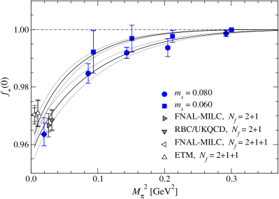
Figure 6: Chiral extrapolation of f+(0)subscript𝑓0f_{+}(0) as a function of Mπ2superscriptsubscript𝑀𝜋2M_{\pi}^{2}. Solid circles and squares show our data at ms=0.080subscript𝑚𝑠0.080m_{s}\!=\!0.080 and 0.060, respectively, whereas the solid diamond represents the value extrapolated to the physical point (ml,phys,ms,phys)subscript𝑚𝑙physsubscript𝑚𝑠phys(m_{l,\rm phys},m_{s,\rm phys}). We note that the physical strange quark mass ms,physsubscript𝑚𝑠physm_{s,\rm phys} (diamond) is slightly off the simulated values (solid lines). We also plot recent results for Nf=2+1subscript𝑁𝑓21N_{f}\!=\!2+1 Kl3:Nf3:FNAL+MILC ; Kl3:Nf3:RBC/UKQCD (shaded symbols) and Nf=2+1+1subscript𝑁𝑓211N_{f}\!=\!2+1+1 Kl3:Nf4:FNAL+MILC ; Kl3:Nf4:ETM (open symbols).

The Ademollo-Gatto theorem Behrends-Sirlin ; Ademollo-Gatto states that SU(3) breaking effects in f+(t)subscript𝑓𝑡f_{+}(t) is second order in (msml)subscript𝑚𝑠subscript𝑚𝑙(m_{s}\!-\!m_{l}) at t=0𝑡0t\!=\!0. The chiral expansion (28) – (37) is reduced into a simpler form with

f+,2,L(0)subscript𝑓2𝐿0\displaystyle f_{+,2,L}(0) =\displaystyle= 0,0\displaystyle 0, (58)
f+,2,B(0)subscript𝑓2𝐵0\displaystyle f_{+,2,B}(0) =\displaystyle= 32HKπ+32HKη,32subscript𝐻𝐾𝜋32subscript𝐻𝐾𝜂\displaystyle\frac{3}{2}H_{K\pi}+\frac{3}{2}H_{K\eta}, (59)
f+,4,C(0)subscript𝑓4𝐶0\displaystyle f_{+,4,C}(0) =\displaystyle= 8c+,πKr(MK2Mπ2)2,8superscriptsubscript𝑐𝜋𝐾𝑟superscriptsuperscriptsubscript𝑀𝐾2superscriptsubscript𝑀𝜋22\displaystyle-8{c_{+,\pi K}^{r}}(M_{K}^{2}-M_{\pi}^{2})^{2}, (60)

where

HPQsubscript𝐻𝑃𝑄\displaystyle H_{PQ} =\displaystyle= 1128π2Fπ2{MP2+MQ22MP2MQ2MP2MQ2ln[MP2MQ2]}.1128superscript𝜋2superscriptsubscript𝐹𝜋2superscriptsubscript𝑀𝑃2superscriptsubscript𝑀𝑄22superscriptsubscript𝑀𝑃2superscriptsubscript𝑀𝑄2superscriptsubscript𝑀𝑃2superscriptsubscript𝑀𝑄2superscriptsubscript𝑀𝑃2superscriptsubscript𝑀𝑄2\displaystyle-\frac{1}{128\pi^{2}F_{\pi}^{2}}\left\{M_{P}^{2}+M_{Q}^{2}-\frac{2M_{P}^{2}M_{Q}^{2}}{M_{P}^{2}-M_{Q}^{2}}\ln\left[\frac{M_{P}^{2}}{M_{Q}^{2}}\right]\right\}. (61)

In previous lattice studies, therefore, one often determines f+(0)subscript𝑓0f_{+}(0) at simulated quark masses by assuming a phenomenological parametrization of the t𝑡t dependence of the form factors, and then extrapolates f+(0)subscript𝑓0f_{+}(0) to the physical point (ml,phys,ms,phys)subscript𝑚𝑙physsubscript𝑚𝑠phys(m_{l,\rm phys},m_{s,\rm phys}) based on NLO or NNLO ChPT.

Table 5: Numerical results of NNLO ChPT fits to form factors. The first line shows results of the conventional fit to f+(0)subscript𝑓0f_{+}(0) in terms of the NG boson masses M{π,K}2superscriptsubscript𝑀𝜋𝐾2M_{\{\pi,K\}}^{2}. The second (third) line is from the fit to f+(t)subscript𝑓𝑡f_{+}(t) (f+(t)subscript𝑓𝑡f_{+}(t) and f~0(t)subscript~𝑓0𝑡\tilde{f}_{0}(t)) in terms of M{π,K}2superscriptsubscript𝑀𝜋𝐾2M_{\{\pi,K\}}^{2} and t𝑡t. The first error is statistical. The second and third are systematics due to the choice of the input Lirsuperscriptsubscript𝐿𝑖𝑟L_{i}^{r}, and truncation of the chiral expansion at NNLO. Note c+,πKr=C12r+C34rsuperscriptsubscript𝑐𝜋𝐾𝑟superscriptsubscript𝐶12𝑟superscriptsubscript𝐶34𝑟{c_{+,\pi K}^{r}}\!=\!C_{12}^{r}+C_{34}^{r} (Eq.(34)).
fit data f+(0)subscript𝑓0f_{+}(0) c+,πKr×105superscriptsubscript𝑐𝜋𝐾𝑟superscript105{c_{+,\pi K}^{r}}\!\times\!10^{5} C12r×105superscriptsubscript𝐶12𝑟superscript105C_{12}^{r}\!\times\!10^{5} C34r×105superscriptsubscript𝐶34𝑟superscript105C_{34}^{r}\!\times\!10^{5}
f+(0)subscript𝑓0f_{+}(0) 0.9636(40)()6+42(+79)0.9636(40)\left({}^{+42}_{-6}\right)(+79) 0.53(7)(6)(17)0.5376170.53(7)(-6)(-17)
f+(t)subscript𝑓𝑡f_{+}(t) 0.9691(42)()5+45(45)0.9691(42)\left({}^{+45}_{-5}\right)(-45) 0.429(73)()71+5(+90)0.429(73)\left({}^{+5}_{-71}\right)(+90)
f+(t)subscript𝑓𝑡f_{+}(t), f~0(t)subscript~𝑓0𝑡\tilde{f}_{0}(t) 0.9636(36)()4+41()19+280.9636(36)\left({}^{+41}_{-4}\right)\left({}^{+28}_{-19}\right) 0.524(62)()80+1()58+330.524(62)\left({}^{+1}_{-80}\right)\left({}^{+33}_{-58}\right) 0.23(7)()13+34()93+5-0.23(7)\left({}^{+34}_{-13}\right)\left({}^{+5}_{-93}\right) 0.76(11)()42+9()11+950.76(11)\left({}^{+9}_{-42}\right)\left({}^{+95}_{-11}\right)

We carry out this type of the conventional analysis using the data of f+(0)subscript𝑓0f_{+}(0) in Table 2. As plotted in Fig. 6, the data are well described by the NNLO ChPT formula with a good value of χ2/d.o.f.0.2\chi^{2}/{\rm d.o.f.}\!\sim\!0.2. Numerical fit results are summarized in Table 5. We observe good agreement in f+(0)subscript𝑓0f_{+}(0) at the physical point (ml,phys,ms,phys)subscript𝑚𝑙physsubscript𝑚𝑠phys(m_{l,\rm phys},m_{s,\rm phys}) with recent lattice studies Kl3:Nf3:FNAL+MILC ; Kl3:Nf4:FNAL+MILC ; Kl3:Nf3:RBC/UKQCD ; Kl3:Nf4:ETM .

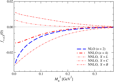
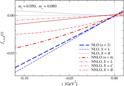
The chiral expansion has reasonable convergence f+(0)=0.9636(40)=10.02320.0132(40)subscript𝑓00.96364010.02320.013240f_{+}(0)\!=\!0.9636(40)\!=\!1-0.0232-0.0132(40) at the physical point. However, Fig. 7 shows that the NLO and NNLO contributions, f+,2(0)subscript𝑓20f_{+,2}(0) and f+,4(0)subscript𝑓40f_{+,4}(0), are comparable at unphysically heavy Mπ300similar-tosubscript𝑀𝜋300M_{\pi}\!\sim\!300 – 500 MeV, and there is a significant cancellation between the analytic (f+,4,C(0)subscript𝑓4𝐶0f_{+,4,C}(0)) and non-analytic (f+,4,L(0)subscript𝑓4𝐿0f_{+,4,L}(0) and f+,4,B(0)subscript𝑓4𝐵0f_{+,4,B}(0)) NNLO contributions.

Refer to caption
Figure 7: LEC-(in)dependent NLO and NNLO contributions to f+(0)subscript𝑓0f_{+}(0). Thick dashed and dot-dashed lines are the NLO and NNLO contributions, whereas the NNLO terms, f+,4,L(0)subscript𝑓4𝐿0f_{+,4,L}(0), f+,4,C(0)subscript𝑓4𝐶0f_{+,4,C}(0) and f+,4,B(0)subscript𝑓4𝐵0f_{+,4,B}(0), are plotted by the thin dot-dot-dashed, dot-dashed and dot-dashed-dashed lines, respectively.
Refer to caption
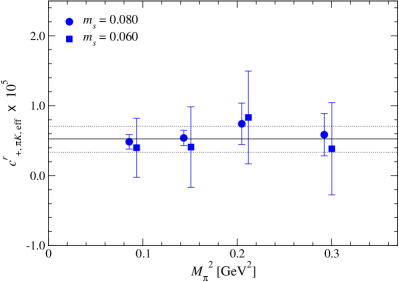
Figure 8: Effective value c+,πK,effrsuperscriptsubscript𝑐𝜋𝐾eff𝑟{c_{+,\pi K,\rm eff}^{r}} as a function of Mπ2superscriptsubscript𝑀𝜋2M_{\pi}^{2}. Squares are slightly shifted along the horizontal axis for clarity. The solid and dotted lines show c+,πKrsuperscriptsubscript𝑐𝜋𝐾𝑟{c_{+,\pi K}^{r}} obtained from the NNLO chiral fit and its uncertainty.

In order to estimate the systematic error due to neglected higher order corrections, we also test a fitting form including a N3LO analytic term f+,6=d+Mπ2(MK2Mπ2)2/Fπ6subscript𝑓6subscript𝑑superscriptsubscript𝑀𝜋2superscriptsuperscriptsubscript𝑀𝐾2superscriptsubscript𝑀𝜋22superscriptsubscript𝐹𝜋6f_{+,6}\!=\!{d_{+}}\,M_{\pi}^{2}\,(M_{K}^{2}-M_{\pi}^{2})^{2}/F_{\pi}^{6}, where the factor (MK2Mπ2)2superscriptsuperscriptsubscript𝑀𝐾2superscriptsubscript𝑀𝜋22(M_{K}^{2}-M_{\pi}^{2})^{2} is motivated by the Ademollo-Gatto theorem. However, the coefficient d+=1.1(1.6)×106subscript𝑑1.11.6superscript106{d_{+}}\!=\!-1.1(1.6)\!\times\!10^{6} is poorly determined, and the extrapolated value f+(0)=0.971(13)subscript𝑓00.97113f_{+}(0)\!=\!0.971(13) is statistically consistent with that from the NNLO fit. This observation and the good value of χ2/d.o.f.formulae-sequencesuperscript𝜒2dof\chi^{2}/{\rm d.o.f.} for the NNLO fit suggest that the uncertainty due to the truncation of the chiral expansion at NNLO is not large compared to the statistical accuracy. We treat the difference in f+(0)subscript𝑓0f_{+}(0) between the fits with and without the N3LO term as a systematic uncertainty in Table 5.
We can examine the significance of the higher order correction without assuming the form of f+,6subscript𝑓6f_{+,6}. Let us consider a quantity

Δf(0)Δ𝑓0\displaystyle\Delta f(0) =\displaystyle= f+(0)f+,0f+,2,L(0)f+,2,B(0)f+,4,L(0)f+,4,B(0),subscript𝑓0subscript𝑓0subscript𝑓2𝐿0subscript𝑓2𝐵0subscript𝑓4𝐿0subscript𝑓4𝐵0\displaystyle f_{+}(0)-f_{+,0}-f_{+,2,L}(0)-f_{+,2,B}(0)-f_{+,4,L}(0)-f_{+,4,B}(0), (62)

which is the sum of the NNLO analytic term and the possible higher order correction f+,4,C(0)+f+,6(0)subscript𝑓4𝐶0subscript𝑓60f_{+,4,C}(0)\!+\!f_{+,6}(0). Note that f+,0(0)subscript𝑓00f_{+,0}(0), f+,2,B(0)subscript𝑓2𝐵0f_{+,2,B}(0) and f+,4,B(0)subscript𝑓4𝐵0f_{+,4,B}(0) are LEC-free in ξ𝜉\xi-expansion, and hence ΔfΔ𝑓\Delta f can be calculated from our data of f+(0)subscript𝑓0f_{+}(0) and inputs in Tables 3. We can define an effective value of c+,πKr=C12r+C34rsuperscriptsubscript𝑐𝜋𝐾𝑟superscriptsubscript𝐶12𝑟superscriptsubscript𝐶34𝑟{c_{+,\pi K}^{r}}\!=\!C_{12}^{r}+C_{34}^{r} as

c+,πK,effrsuperscriptsubscript𝑐𝜋𝐾eff𝑟\displaystyle{c_{+,\pi K,\rm eff}^{r}} =\displaystyle= Fπ48(MK2Mπ2)2Δf=c+,πKr+O(Mπ2,MK2),superscriptsubscript𝐹𝜋48superscriptsuperscriptsubscript𝑀𝐾2superscriptsubscript𝑀𝜋22Δ𝑓superscriptsubscript𝑐𝜋𝐾𝑟𝑂superscriptsubscript𝑀𝜋2superscriptsubscript𝑀𝐾2\displaystyle-\frac{F_{\pi}^{4}}{8(M_{K}^{2}-M_{\pi}^{2})^{2}}\Delta f={c_{+,\pi K}^{r}}+O(M_{\pi}^{2},M_{K}^{2}), (63)

which deviates from c+,πKrsuperscriptsubscript𝑐𝜋𝐾𝑟{c_{+,\pi K}^{r}} and shows a non-trivial quark mass dependence, if the higher order correction f+,6subscript𝑓6f_{+,6} is significant in the simulation region. As shown in Fig. 8, however, our result has small dependence on mlsubscript𝑚𝑙m_{l} and mssubscript𝑚𝑠m_{s} suggesting that the higher order correction is not large compared to the statistical accuracy.
Refer to caption
Refer to caption
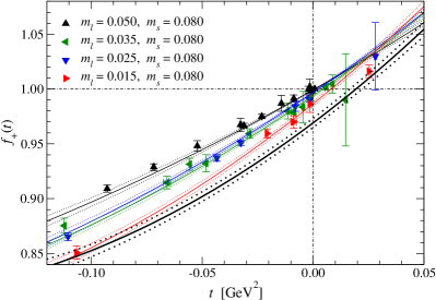
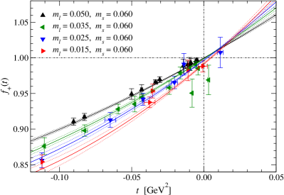
Figure 9: Chiral extrapolation of f+(t)subscript𝑓𝑡f_{+}(t) as a function of t𝑡t. Different symbols show data at different values of mlsubscript𝑚𝑙m_{l}, whereas the left and right panels are for ms=0.080subscript𝑚𝑠0.080m_{s}\!=\!0.080 and 0.060, respectively. Thin solid and dotted lines show the fit curve and its statistical uncertainty. We also plot those at the physical point (ml,phys,ms,phys)subscript𝑚𝑙physsubscript𝑚𝑠phys(m_{l,\rm phys},m_{s,\rm phys}) by thick lines in the left panel at msms,physsimilar-tosubscript𝑚𝑠subscript𝑚𝑠physm_{s}\!\sim\!m_{s,\rm phys}.

It is advantageous to use not only f+(0)subscript𝑓0f_{+}(0) but all the data of f+(t)subscript𝑓𝑡f_{+}(t) to better constrain the possible higher order chiral corrections. Parametrizing both the t𝑡t and quark mass dependences based on ChPT reduces the model dependence of our analysis. We therefore carry out a fit for f+(t)subscript𝑓𝑡f_{+}(t) using the chiral expansion (28) as a function of t𝑡t, Mπ2superscriptsubscript𝑀𝜋2M_{\pi}^{2} and MK2superscriptsubscript𝑀𝐾2M_{K}^{2}. As shown in Fig. 9, the t𝑡t dependence of our data is also described well by the NNLO formula with an acceptable value of χ/d.o.f.0.7\chi/{\rm d.o.f.}\!\sim\!0.7, because we simulate a limited region of t0similar-to𝑡0t\!\sim\!0.

Results for the LEC c+,πKrsuperscriptsubscript𝑐𝜋𝐾𝑟{c_{+,\pi K}^{r}} and the normalization f+(0)subscript𝑓0f_{+}(0) at the physical point in Table 5 show good consistency with those from the conventional analysis. Their systematic error due to the truncation of the chiral expansion at NNLO is estimated by repeating the fit with each of the following higher order terms

Fπ6f+,6superscriptsubscript𝐹𝜋6subscript𝑓6\displaystyle F_{\pi}^{6}\,f_{+,6} =\displaystyle= d+Mπ2(MK2Mπ2)2,d+Mπ4t,d+Mπ2t2,d+Mπ2MK2t.subscript𝑑superscriptsubscript𝑀𝜋2superscriptsuperscriptsubscript𝑀𝐾2superscriptsubscript𝑀𝜋22subscript𝑑superscriptsubscript𝑀𝜋4𝑡subscript𝑑superscriptsubscript𝑀𝜋2superscript𝑡2subscript𝑑superscriptsubscript𝑀𝜋2superscriptsubscript𝑀𝐾2𝑡\displaystyle{d_{+}}M_{\pi}^{2}(M_{K}^{2}-M_{\pi}^{2})^{2},\hskip 8.53581pt{d_{+}}M_{\pi}^{4}t,\hskip 8.53581pt{d_{+}}M_{\pi}^{2}t^{2},\hskip 8.53581pt{d_{+}}M_{\pi}^{2}M_{K}^{2}t. (64)

This uncertainty is slightly smaller than the conventional analysis, because the coefficient d+subscript𝑑{d_{+}} is better constrained with more data at non-zero t𝑡t’s.

Refer to caption
Refer to caption
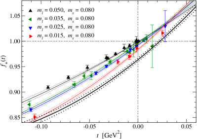
Figure 10: Simultaneous chiral fit to f+(t)subscript𝑓𝑡f_{+}(t) (left panel) and f~0(t)subscript~𝑓0𝑡\tilde{f}_{0}(t) (right panel) at ms=0.080subscript𝑚𝑠0.080m_{s}\!=\!0.080. Data at different values of mlsubscript𝑚𝑙m_{l} are plotted by different symbols as a function of t𝑡t. Thin solid and dotted line shows the fit curve and the statistical uncertainty, whereas thick lines show those at (ml,phys,ms,phys)subscript𝑚𝑙physsubscript𝑚𝑠phys(m_{l,\rm phys},m_{s,\rm phys}).

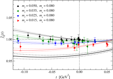
In order to make use of all the available data, we performed a simultaneous fit to f+(t)subscript𝑓𝑡f_{+}(t) and f~0(t)subscript~𝑓0𝑡\tilde{f}_{0}(t) as a function of t𝑡t, Mπ2superscriptsubscript𝑀𝜋2M_{\pi}^{2} and MK2superscriptsubscript𝑀𝐾2M_{K}^{2}. As shown in Fig. 10, the NNLO formulae (28) and (54) describe our data well with a good value of χ2/d.o.f.0.7\chi^{2}/{\rm d.o.f.}\!\sim\!0.7. Numerical results of the fit are summarized in Table 5. We estimate the uncertainty due to possible higher order corrections by testing the N3LO terms (64) for f+,6subscript𝑓6f_{+,6} and the followings for f~0,6subscript~𝑓06\tilde{f}_{0,6}

Fπ6f~0,6superscriptsubscript𝐹𝜋6subscript~𝑓06\displaystyle F_{\pi}^{6}\,\tilde{f}_{0,6} =\displaystyle= d+Mπ2(MK2Mπ2)2,d0Mπ4t,d0Mπ2t2,d0Mπ2MK2t.subscript𝑑superscriptsubscript𝑀𝜋2superscriptsuperscriptsubscript𝑀𝐾2superscriptsubscript𝑀𝜋22subscript𝑑0superscriptsubscript𝑀𝜋4𝑡subscript𝑑0superscriptsubscript𝑀𝜋2superscript𝑡2subscript𝑑0superscriptsubscript𝑀𝜋2superscriptsubscript𝑀𝐾2𝑡\displaystyle{d_{+}}M_{\pi}^{2}(M_{K}^{2}-M_{\pi}^{2})^{2},\hskip 8.53581pt{d_{0}}M_{\pi}^{4}t,\hskip 8.53581pt{d_{0}}M_{\pi}^{2}t^{2},\hskip 8.53581pt{d_{0}}M_{\pi}^{2}M_{K}^{2}t. (65)

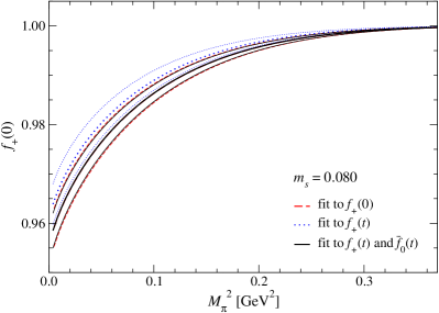
Table 5 shows good consistency in c+,πKrsuperscriptsubscript𝑐𝜋𝐾𝑟{c_{+,\pi K}^{r}} and f+(0)subscript𝑓0f_{+}(0) at the physical point among the three types of the chiral fit: namely, the fit to f+(0)subscript𝑓0f_{+}(0), that to f+(t)subscript𝑓𝑡f_{+}(t), and the simultaneous fit to f+(t)subscript𝑓𝑡f_{+}(t) and f~0(t)subscript~𝑓0𝑡\tilde{f}_{0}(t). This is also demonstrated in Fig. 11, where the Mπsubscript𝑀𝜋M_{\pi} dependence of f+(0)subscript𝑓0f_{+}(0) at ms=0.080ms,physsubscript𝑚𝑠0.080similar-tosubscript𝑚𝑠physm_{s}\!=\!0.080\!\sim\!m_{s,\rm phys} is reproduced from the three fits. We observe good agreement within 1σsimilar-toabsent1𝜎\sim\!1~{}\sigma in the whole simulation region of Mπ2superscriptsubscript𝑀𝜋2M_{\pi}^{2}.

Refer to caption
Figure 11: Comparison of fit curves for f+(0)subscript𝑓0f_{+}(0) at ms=0.080ms,physsubscript𝑚𝑠0.080similar-tosubscript𝑚𝑠physm_{s}\!=\!0.080\!\sim\!m_{s,\rm phys}. The dashed, dotted and solid lines lines are reproduced from the fits to f+(0)subscript𝑓0f_{+}(0), f+(t)subscript𝑓𝑡f_{+}(t) and the simultaneous fit to f+(t)subscript𝑓𝑡f_{+}(t) and f~0(t)subscript~𝑓0𝑡\tilde{f}_{0}(t), respectively. For each fit, the thick line shows the central value, whereas its statistical error is shown by the two thin lines.

Table 5 shows that the statistical accuracy of the fit results is not largely different between the conventional fit and the fit to f+subscript𝑓f_{+}. Indeed, these two fits use the same data of f+subscript𝑓f_{+} but different parametrizations for the t𝑡t dependence: Eq. (25) or ChPT. The statistical error is slightly reduced by using f~0subscript~𝑓0\tilde{f}_{0}. The uncertainty due to the choice of the input (Tables 3 and 4) is more or less the same among the three fits. However, the uncertainty due to the truncation of the chiral expansion is significantly reduced by including more data into the ChPT fit. From this observation, we consider the simultaneous fit to f+subscript𝑓f_{+} and f~0subscript~𝑓0\tilde{f}_{0} as our best fit.

Refer to caption
Refer to caption
Refer to caption
Refer to caption
Refer to caption
Refer to caption
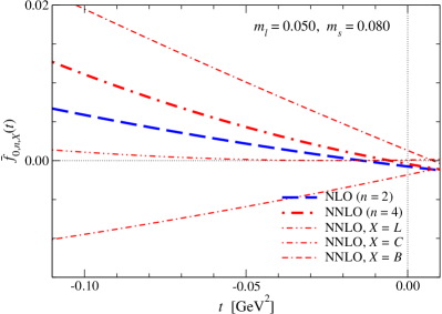
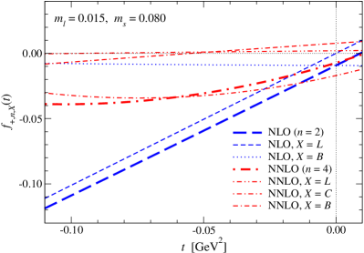
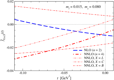
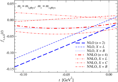
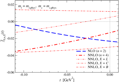
Figure 12: LEC-(in)dependent NLO and NNLO contributions to f+(t)subscript𝑓𝑡f_{+}(t) (left panels) and f~0(t)subscript~𝑓0𝑡\tilde{f}_{0}(t) (right panels) as a function of t𝑡t. The top, middle and bottom panels show data at (ml,ms)=(0.050,0.080)subscript𝑚𝑙subscript𝑚𝑠0.0500.080(m_{l},m_{s})\!=\!(0.050,0.080), (0.015,0.080) and the physical point (ml,phys,ms,phys)subscript𝑚𝑙physsubscript𝑚𝑠phys(m_{l,\rm phys},m_{s,\rm phys}), respectively. The net NLO and NNLO contributions are plotted by thick blue dashed and red dot-dashed lines, respectively. Thin lines show their breakdown into LEC-(in)dependent terms.

We investigate the convergence of this best fit in Fig. 12. Our observations on f+subscript𝑓f_{+} at large space-like momentum transfer t0much-greater-than𝑡0-t\!\gg\!0 are similar to those on the charged meson EM form factors FV{π+,K+}superscriptsubscript𝐹𝑉superscript𝜋superscript𝐾F_{V}^{\{\pi^{+},K^{+}\}} in Ref. EMFF:JLQCD:Nf3:RG+Ovr . The analytic term f+,2,Lsubscript𝑓2𝐿f_{+,2,L} (f+,4,Csubscript𝑓4𝐶f_{+,4,C}) is dominant NLO (largest NNLO) contribution to f+,2subscript𝑓2f_{+,2} (f+,4subscript𝑓4f_{+,4}). We note that our estimate of the relevant LECs in Tables 3 – 5 is not unexpectedly large, and consistent with an order estimate ChPT:LECs:SU2+SU3

Lir=O((4π)2)=O(6×10³),Cir=O((4π)4)=O(4×10⁵).formulae-sequencesuperscriptsubscript𝐿𝑖𝑟𝑂superscript4𝜋2𝑂6superscript103superscriptsubscript𝐶𝑖𝑟𝑂superscript4𝜋4𝑂4superscript105\displaystyle L_{i}^{r}=O((4\pi)^{-2})=O(6\!\times\!10^{-3}),\hskip 14.22636ptC_{i}^{r}=O((4\pi)^{-4})=O(4\!\times\!10^{-5}). (66)

The large analytic terms, f+,2,Lsubscript𝑓2𝐿f_{+,2,L} and f+,4,Csubscript𝑓4𝐶f_{+,4,C}, suggest the importance of the first-principle determination of the relevant LECs. While we employ the input in Table 3 for other LECs involved in f+,4,Lsubscript𝑓4𝐿f_{+,4,L}, this term turns out to be small. Therefore, the systematic uncertainty due to the choice of the input is not large.

The convergence at t0much-greater-than𝑡0-t\!\gg\!0 is reasonably good and becomes better toward smaller Mπsubscript𝑀𝜋M_{\pi}. This is because the dominant NLO term f+,2,Lt/Fπ2proportional-tosubscript𝑓2𝐿𝑡superscriptsubscript𝐹𝜋2f_{+,2,L}\!\propto\!t/F_{\pi}^{2} is not suppressed by the NG boson masses and even enhanced by the factor Fπ2superscriptsubscript𝐹𝜋2F_{\pi}^{-2} in the ξ𝜉\xi-expansion. A similar convergence property is also observed for the EM form factors FV{π+,K+}superscriptsubscript𝐹𝑉superscript𝜋superscript𝐾F_{V}^{\{\pi^{+},K^{+}\}} EMFF:JLQCD:Nf3:RG+Ovr .

There is a property of f+subscript𝑓f_{+} different from FV{π+,K+}superscriptsubscript𝐹𝑉superscript𝜋superscript𝐾F_{V}^{\{\pi^{+},K^{+}\}} near the important reference point t=0𝑡0t\!=\!0. Unless mlmssubscript𝑚𝑙subscript𝑚𝑠m_{l}\!\neq\!m_{s}, each chiral correction does not necessarily vanish except f+,2,Lsubscript𝑓2𝐿f_{+,2,L}, which is dominantly large at t0much-greater-than𝑡0-t\!\gg\!0 (blue thin dashed lines in Fig. 12). As a result, the chiral expansion has a poorer convergence towards t=0𝑡0t\!=\!0 as already observed in Fig. 7. Note, however, that our analysis in Fig. 8 does not suggest statistically significant N3LO nor higher order corrections.

In our analysis, the quantity f~0subscript~𝑓0\tilde{f}_{0} is used to obtain additional constraints on the relevant O(p6)𝑂superscript𝑝6O(p^{6}) couplings, C12rsuperscriptsubscript𝐶12𝑟C_{12}^{r} and C34rsuperscriptsubscript𝐶34𝑟C_{34}^{r}. For this purpose, f~0subscript~𝑓0\tilde{f}_{0} is designed to have no NLO analytic term, which is a dominant contribution to f+subscript𝑓f_{+}, and its dependence on Lirsuperscriptsubscript𝐿𝑖𝑟L_{i}^{r} starts from NNLO. The right panels of Fig. 12 show that the Lisubscript𝐿𝑖L_{i}-dependent NNLO correction f~0,4,Lsubscript~𝑓04𝐿\tilde{f}_{0,4,L} is not large with our choice of the input in Table 3. The remaining loop corrections, f~0,2,Bsubscript~𝑓02𝐵\tilde{f}_{0,2,B} and f~0,4,Bsubscript~𝑓04𝐵\tilde{f}_{0,4,B}, are parameter-free in the ξ𝜉\xi-expansion. Therefore, f~0subscript~𝑓0\tilde{f}_{0} has reasonable sensitivity to the NNLO analytic term f~0,4,Csubscript~𝑓04𝐶\tilde{f}_{0,4,C}. This leads to our observation in Table 5: incorporating f~0subscript~𝑓0\tilde{f}_{0} into the chiral extrapolation is helpful in improving the statistical accuracy of c+,πKrsuperscriptsubscript𝑐𝜋𝐾𝑟{c_{+,\pi K}^{r}} and f+(0)subscript𝑓0f_{+}(0), and also in reducing their systematic error due to the truncation of the chiral expansion.

For phenomenological applications, it is preferable to separately fix C12rsuperscriptsubscript𝐶12𝑟C_{12}^{r} and C34rsuperscriptsubscript𝐶34𝑟C_{34}^{r} rather than their sum c+,πKrsuperscriptsubscript𝑐𝜋𝐾𝑟{c_{+,\pi K}^{r}}. This is only possible with the data of f~0subscript~𝑓0\tilde{f}_{0} by disentangle their Mπ2superscriptsubscript𝑀𝜋2M_{\pi}^{2}, MK2superscriptsubscript𝑀𝐾2M_{K}^{2} and t𝑡t dependences in the NNLO correction (57). As mentioned above, however, f~0subscript~𝑓0\tilde{f}_{0} is designed to have the small NLO correction f~0,2subscript~𝑓02\tilde{f}_{0,2}. This quantity is sensitive to not only NNLO but the even higher order corrections (64) and (65) added by hand to estimate the systematic uncertainty due to the truncation of the chiral expansion. As a result, this uncertainty for C12rsuperscriptsubscript𝐶12𝑟C_{12}^{r} and C34rsuperscriptsubscript𝐶34𝑟C_{34}^{r} is rather large in Table 5. In this study, therefore, we only confirm that our results are consistent with the order estimate (66). We note that a better determination of C12rsuperscriptsubscript𝐶12𝑟C_{12}^{r} and C34rsuperscriptsubscript𝐶34𝑟C_{34}^{r} needs more data of f~0subscript~𝑓0\tilde{f}_{0} at smaller values of Mπsubscript𝑀𝜋M_{\pi} and MKsubscript𝑀𝐾M_{K}.

IV.3 Form factor shape

In order to support the reliability of the determination of f+(0)subscript𝑓0f_{+}(0) with the sub-percent level accuracy, it is important to check the consistency of the form factors’ shape on the lattice with experiments. In recent analyses of experimental data, it is popular to employ the so-called dispersive parametrization of the t𝑡t dependence shape:disp:scalar ; shape:disp:vector based on the analyticity of the form factors. In this study, however, we consider the slope λ{+,0}superscriptsubscript𝜆0\lambda_{\{+,0\}}^{\prime} in the conventional quadratic parametrization (26). These are convenient in our analysis based on ChPT, since the chiral expansion is the expansion in terms of t𝑡t (and the NG boson masses). We note that the quadratic parametrization has been also well studied phenomenologically and experimentally. Its relation to the dispersive one has been established shape:disp:vector . From recent experimental data CKM16:Moulson , the slopes are estimated as

λ+=2.58(7)×102,λ0=1.36(7)×102.formulae-sequencesuperscriptsubscript𝜆2.587superscript102superscriptsubscript𝜆01.367superscript102\displaystyle\lambda_{+}^{\prime}=2.58(7)\times 10^{-2},\hskip 14.22636pt\lambda_{0}^{\prime}=1.36(7)\times 10^{-2}. (67)

In this paper, we treat Mπ±2superscriptsubscript𝑀superscript𝜋plus-or-minus2M_{\pi^{\pm}}^{2} in Eq. (26) just as the normalization factor to make λ{+,0}subscript𝜆0\lambda_{\{+,0\}} dimensionless, and fix it to its physical value. The slope is then given as

λ{+,0}superscriptsubscript𝜆0\displaystyle\lambda_{\{+,0\}}^{\prime} =\displaystyle= Mπ±,phys2f{+,0}(0)df{+,0}(t)dt|t=0.evaluated-atsuperscriptsubscript𝑀superscript𝜋plus-or-minusphys2subscript𝑓00𝑑subscript𝑓0𝑡𝑑𝑡𝑡0\displaystyle\left.\frac{M_{\pi^{\pm},\rm phys}^{2}}{f_{\{+,0\}}(0)}\frac{df_{\{+,0\}}(t)}{dt}\right|_{t=0}. (68)

We evaluate both the normalization f+(0)=f0(0)subscript𝑓0subscript𝑓00f_{+}(0)\!=\!f_{0}(0) (Table 5) and derivatives df{+,0}/dt|t=0evaluated-at𝑑subscript𝑓0𝑑𝑡𝑡0df_{\{+,0\}}/dt|_{t=0} from our chiral fit of f+subscript𝑓f_{+} and f~0subscript~𝑓0\tilde{f}_{0} based on NNLO ChPT.

It is straightforward to calculate df+/dt|t=0evaluated-at𝑑subscript𝑓𝑑𝑡𝑡0df_{+}/dt|_{t=0}. From the chiral expansion (28), (29) and (32), it is given as

df+(t)dt𝑑subscript𝑓𝑡𝑑𝑡\displaystyle\frac{df_{+}(t)}{dt} =\displaystyle= df+,2(t)dt+df+,4(t)dt+df+,6(t)dt,𝑑subscript𝑓2𝑡𝑑𝑡𝑑subscript𝑓4𝑡𝑑𝑡𝑑subscript𝑓6𝑡𝑑𝑡\displaystyle\frac{df_{+,2}(t)}{dt}+\frac{df_{+,4}(t)}{dt}+\frac{df_{+,6}(t)}{dt}, (69)
df+,2(t)dt𝑑subscript𝑓2𝑡𝑑𝑡\displaystyle\frac{df_{+,2}(t)}{dt} =\displaystyle= df+,2,L(t)dt+df+,2,B(t)dt,𝑑subscript𝑓2𝐿𝑡𝑑𝑡𝑑subscript𝑓2𝐵𝑡𝑑𝑡\displaystyle\frac{df_{+,2,L}(t)}{dt}+\frac{df_{+,2,B}(t)}{dt}, (70)
df+,4(t)dt𝑑subscript𝑓4𝑡𝑑𝑡\displaystyle\frac{df_{+,4}(t)}{dt} =\displaystyle= df+,4,C(t)dt+df+,4,L(t)dt+df+,4,B(t)dt.𝑑subscript𝑓4𝐶𝑡𝑑𝑡𝑑subscript𝑓4𝐿𝑡𝑑𝑡𝑑subscript𝑓4𝐵𝑡𝑑𝑡\displaystyle\frac{df_{+,4,C}(t)}{dt}+\frac{df_{+,4,L}(t)}{dt}+\frac{df_{+,4,B}(t)}{dt}. (71)

The derivatives of f+,2,Lsubscript𝑓2𝐿f_{+,2,L}, f+,2,Bsubscript𝑓2𝐵f_{+,2,B}, f+,4,Csubscript𝑓4𝐶f_{+,4,C} and f+,6subscript𝑓6f_{+,6} are analytically calculable from their expressions (30), (31), (33) and (64). Since the NNLO non-analytic terms, f+,4,Lsubscript𝑓4𝐿f_{+,4,L} and f+,4,Bsubscript𝑓4𝐵f_{+,4,B}, have rather lengthy expressions, we numerically evaluate their derivatives as in our study of the light meson charge radii EMFF:JLQCD:Nf3:RG+Ovr .

We evaluate df0/dt|t=0evaluated-at𝑑subscript𝑓0𝑑𝑡𝑡0df_{0}/dt|_{t=0} through

df0(t)dt𝑑subscript𝑓0𝑡𝑑𝑡\displaystyle\frac{df_{0}(t)}{dt} =\displaystyle= df~0(t)dt1MK2Mπ2(1FKFπ).𝑑subscript~𝑓0𝑡𝑑𝑡1superscriptsubscript𝑀𝐾2superscriptsubscript𝑀𝜋21subscript𝐹𝐾subscript𝐹𝜋\displaystyle\frac{d\tilde{f}_{0}(t)}{dt}-\frac{1}{M_{K}^{2}-M_{\pi}^{2}}\left(1-\frac{F_{K}}{F_{\pi}}\right). (72)

Here df~0/dt|t=0evaluated-at𝑑subscript~𝑓0𝑑𝑡𝑡0d\tilde{f}_{0}/dt|_{t=0} is calculated in a similar way to df+/dt|t=0evaluated-at𝑑subscript𝑓𝑑𝑡𝑡0df_{+}/dt|_{t=0}, whereas FK/Fπsubscript𝐹𝐾subscript𝐹𝜋F_{K}/F_{\pi} is estimated from our NNLO chiral fit in Ref. Spectrum:Nf3:RG+Ovr:JLQCD .
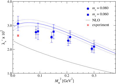
Refer to caption
Refer to caption
Figure 13: Slope parameters λ+superscriptsubscript𝜆\lambda_{+}^{\prime} (left panel) and λ0superscriptsubscript𝜆0\lambda_{0}^{\prime} (right panel) as a function of Mπ2superscriptsubscript𝑀𝜋2M_{\pi}^{2}. The blue solid and dotted lines are reproduced from our chiral fit based on NNLO ChPT, and represent the slopes at a simulated strange quark mass ms=0.080subscript𝑚𝑠0.080m_{s}\!=\!0.080. The black dashed (dot-dashed) line shows the contribution from the NLO (NNLO) correction to f+subscript𝑓f_{+} and f~0subscript~𝑓0\tilde{f}_{0}. The value extrapolated to the physical point (mud,phys,ms,phys)subscript𝑚𝑢𝑑physsubscript𝑚𝑠phys(m_{ud,\rm phys},m_{s,\rm phys}) is plotted by the blue diamonds, whereas the red stars represent the experimental values (67). We also plot the values in Table 2 by blue circles (ms=0.080subscript𝑚𝑠0.080m_{s}\!=\!0.080) and squares (0.060).

Our results for λ{+,0}superscriptsubscript𝜆0\lambda_{\{+,0\}}^{\prime} are plotted in Fig. 13 as a function of Mπ2superscriptsubscript𝑀𝜋2M_{\pi}^{2}. We observe reasonable agreement with the values in Table 2, which are estimated by assuming the VMD-based parametrization (25) for f+subscript𝑓f_{+} and the quadratic form (26) for f0subscript𝑓0f_{0}. This agreement does not necessarily hold, since the non-analytic chiral behavior is not explicitly taken into account in the model assumptions. The reasonable consistency in λ+superscriptsubscript𝜆\lambda_{+}^{\prime} is therefore compatible with our observation in Fig. 12 that non-analytic corrections to f+subscript𝑓f_{+} are not large at the simulation points.

The dashed line in the left panel of Fig. 13 shows λ+superscriptsubscript𝜆\lambda_{+}^{\prime} up to NLO. The NNLO correction turns out to be significant at the simulation points and down to the physical point. In the whole region, the analytic term f+,4,Csubscript𝑓4𝐶f_{+,4,C} gives rise to a dominant part of the NNLO correction suggesting the importance of the first-principle determination of the relevant LECs. We observe that contribution from the NNLO non-analytic term f+,4,Lsubscript𝑓4𝐿f_{+,4,L} become significant below the simulation points Mπ0.09GeV2less-than-or-similar-tosubscript𝑀𝜋0.09superscriptGeV2M_{\pi}\!\lesssim\!0.09~{}\mbox{GeV}^{2} and leads to the non-monotonous Mπ2superscriptsubscript𝑀𝜋2M_{\pi}^{2} dependence of λ+superscriptsubscript𝜆\lambda_{+}^{\prime}. It is therefore important to study the form factor shape by taking account of the chiral logarithmic terms.

In the right panel of Fig. 13, dashed and dot-dashed lines show contributions to λ0superscriptsubscript𝜆0\lambda_{0}^{\prime} from f~0subscript~𝑓0\tilde{f}_{0}, which are not large. The slope is therefore dominated by the second term in the right-hand side of Eq. (72). This is because a large part of the NLO and NNLO analytic terms, which give rise to a large contribution to λ+superscriptsubscript𝜆\lambda_{+}^{\prime}, are absorbed into the second term. This suggests that a modified version KFF:ChPT:SU3:NLO of the Dashen-Weinstein relation Dashen-Weinstein

f0(0)f0(0)superscriptsubscript𝑓00subscript𝑓00\displaystyle\frac{f_{0}^{\prime}(0)}{f_{0}(0)} =\displaystyle= λ0Mπ±,phys21MK2Mπ2(FKFπ1)similar-tosuperscriptsubscript𝜆0superscriptsubscript𝑀superscript𝜋plus-or-minusphys21superscriptsubscript𝑀𝐾2superscriptsubscript𝑀𝜋2subscript𝐹𝐾subscript𝐹𝜋1\displaystyle\frac{\lambda_{0}^{\prime}}{M_{\pi^{\pm},\rm phys}^{2}}\sim\ \frac{1}{M_{K}^{2}-M_{\pi}^{2}}\left(\frac{F_{K}}{F_{\pi}}-1\right) (73)

holds reasonably well in a wide region of Mπ500less-than-or-similar-tosubscript𝑀𝜋500M_{\pi}\!\lesssim\!500 MeV.

IV.4 Numerical results for form factors and LEC

Our numerical result for the normalization is

f+(0)subscript𝑓0\displaystyle f_{+}(0) =\displaystyle= 0.9636(36)stat()19+49chiral(29)a0.\displaystyle 0.9636(36)_{\rm stat}\left({}^{+49}_{-19}\right)_{\rm chiral}(29)_{a\neq 0}. (74)

The first error is statistical. The second error is due to the chiral extrapolation and is a quadrature sum of the uncertainties from the choice of the input L{1,,8}subscript𝐿18L_{\{1,...,8\}} (Table 3) and the truncation of the chiral expansion at NNLO. The third one represents discretization errors at our finite lattice spacing. Since the LO term f+,0=1subscript𝑓01f_{+,0}\!=\!1 is fixed from symmetry, we assign discretization errors to the non-trivial chiral correction f+,2+f+,4subscript𝑓2subscript𝑓4f_{+,2}+f_{+,4} by an order counting O((aΛQCD)2)8similar-to𝑂superscript𝑎subscriptΛQCD28O((a\Lambda_{\rm QCD})^{2})\!\sim\!8 % with ΛQCD=500subscriptΛQCD500\Lambda_{\rm QCD}\!=\!500 MeV. We expect that f+,2+f+,4subscript𝑓2subscript𝑓4f_{+,2}+f_{+,4} also receives finite volume effects of O(eMπL)1similar-to𝑂superscript𝑒subscript𝑀𝜋𝐿1O(e^{-M_{\pi}L})\!\sim\!1 – 2 %. This is, however, well below other uncertainties.

A latest analysis of available experimental data together with analytic calculations of the isospin and EM corrections CKM16:Moulson ; Kl3:EM:CKNRT ; Kl3:isospin:KN ; Kl3:EM:CGN obtains |Vus|f+(0)=0.21654(41)subscript𝑉𝑢𝑠subscript𝑓00.2165441|V_{us}|f_{+}(0)\!=\!0.21654(41) CKM16:Moulson . Our results leads to

|Vus|subscript𝑉𝑢𝑠\displaystyle|V_{us}| =\displaystyle= 0.2247()12+16th(4)ex,\displaystyle 0.2247\left({}^{+16}_{-12}\right)_{\rm th}(4)_{\rm ex}, (75)

and a measure of the unitarity violation in the first row

ΔCKMsubscriptΔCKM\displaystyle\Delta_{\rm CKM} =\displaystyle= |Vud|2+|Vus|2+|Vub|21=0.0004()8+7.\displaystyle|V_{ud}|^{2}+|V_{us}|^{2}+|V_{ub}|^{2}-1=-0.0004\left({}^{+7}_{-8}\right). (76)

Here we use recent estimate |Vud|=0.97420(21)subscript𝑉𝑢𝑑0.9742021|V_{ud}|\!=\!0.97420(21) CKM16:Hardy from the super-allowed nuclear β𝛽\beta decays. Note that |Vub|4×10³subscript𝑉𝑢𝑏4superscript103|V_{ub}|\!\approx\!4\!\times\!10^{-3} PDG16 is too small to affect this test of CKM unitarity, and the long-standing tension between the exclusive and inclusive decays does not change ΔCKMsubscriptΔCKM\Delta_{\rm CKM} significantly. CKM unitarity fulfilled at the level of O(0.1%)𝑂percent0.1O(0.1\,\%) may have sensitivity to new physics at the TeV scale NPtest:GC .

For the LEC and form factor shape, we obtain

c+,πKr(Mρ)superscriptsubscript𝑐𝜋𝐾𝑟subscript𝑀𝜌\displaystyle{c_{+,\pi K}^{r}}(M_{\rho}) =\displaystyle= C12r(Mρ)+C34r(Mρ)=0.524(62)stat()99+33chiral(42)a0×105,\displaystyle C_{12}^{r}(M_{\rho})+C_{34}^{r}(M_{\rho})=0.524(62)_{\rm stat}\left({}^{+33}_{-99}\right)_{\rm chiral}(42)_{a\neq 0}\times 10^{-5}, (77)
λ+superscriptsubscript𝜆\displaystyle\lambda_{+}^{\prime} =\displaystyle= 3.08(14)stat()4+12chiral(25)a0×102,\displaystyle 3.08(14)_{\rm stat}\left({}^{+12}_{-4}\right)_{\rm chiral}(25)_{a\neq 0}\times 10^{-2}, (78)
λ0superscriptsubscript𝜆0\displaystyle\lambda_{0}^{\prime} =\displaystyle= 1.98(15)stat()41+31chiral(16)a0×102,\displaystyle 1.98(15)_{\rm stat}\left({}^{+31}_{-41}\right)_{\rm chiral}(16)_{a\neq 0}\times 10^{-2}, (79)

where we assign O((aΛQCD)2)𝑂superscript𝑎subscriptΛQCD2O((a\Lambda_{\rm QCD})^{2}) discretization errors, and 1 – 2 % finite volume effects are well below other uncertainties. We note that our chiral fit to f+(0)subscript𝑓0f_{+}(0) and that to f+(t)subscript𝑓𝑡f_{+}(t) yield consistent results for the normalization and LEC. Recent lattice estimate Kl3:Nf3:FNAL+MILC ; Kl3:Nf3:RBC/UKQCD ; Kl3:Nf4:FNAL+MILC ; Kl3:Nf4:ETM and the current world average FLAG3 for f+(0)subscript𝑓0f_{+}(0) are in good agreement with our result. We also observe reasonable consistency with a previous lattice estimate of the LEC c+,πKr(Mρ)=0.46(10)×105superscriptsubscript𝑐𝜋𝐾𝑟subscript𝑀𝜌0.4610superscript105{c_{+,\pi K}^{r}}(M_{\rho})\!=\!0.46(10)\!\times\!10^{-5} Kl3:Nf3:FNAL+MILC and experimental results for the slopes (67).

V Conclusions

In this article, we have presented our study of the chiral behavior of the Kπ𝐾𝜋K\!\to\!\pi semileptonic form factors. Relevant meson correlators are precisely calculated by using the all-to-all quark propagator. Our data of the form factors are directly compared with NNLO ChPT in the continuum limit by exploiting exact chiral symmetry preserved by the overlap quark action.

Similar to our observation in our study of the EM form factors, the non-trivial chiral correction to the vector form factor f+1subscript𝑓1f_{+}\!-\!1 is largely dominated by the NLO analytic term f+,2,Ltproportional-tosubscript𝑓2𝐿𝑡f_{+,2,L}\!\propto\!t. As a result, the NNLO chiral expansion exhibits reasonably good convergence particularly at t0much-less-than𝑡0t\!\ll\!0, and describes our data reasonably well. While f+,2,Lsubscript𝑓2𝐿f_{+,2,L} vanishes and the convergence becomes poorer towards t=0𝑡0t\!=\!0, our analysis suggests that N3LO and even higher order corrections are not large compared to the statistical accuracy.

We determined the normalization f+(0)subscript𝑓0f_{+}(0) within 1absent1\leq\!1 % accuracy from our chiral fit to f+(t)subscript𝑓𝑡f_{+}(t) and f~0(t)subscript~𝑓0𝑡\tilde{f}_{0}(t) based on NNLO ChPT. The result is nicely consistent with CKM unitarity in the first row. We also estimate the relevant O(p6)𝑂superscript𝑝6O(p^{6}) coupling C12r+C34rsuperscriptsubscript𝐶12𝑟superscriptsubscript𝐶34𝑟C_{12}^{r}\!+\!C_{34}^{r} and the slope parameters λ{+,0}superscriptsubscript𝜆0\lambda_{\{+,0\}}^{\prime} from the same fit, and observe reasonable consistency with a previous lattice study and experiments, respectively.

The statistical and systematic uncertainties of f+(0)subscript𝑓0f_{+}(0) turn out to be comparable to each other with our simulation set-up. Its accuracy can be improved in the future by more realistic simulations with higher statistics. Note that the uncertainty of the isospin breaking and EM corrections are typically 0.1 – 0.2%. Good control of these corrections will be increasingly important, as the accuracy of f+(0)subscript𝑓0f_{+}(0) approaches this level.

It is interesting to extend this work to the heavy meson decays to test the Standard Model by a broad range of experimental measurements. Simulations on finer lattices are underway JLQCD:Noaki:Lat14 by using a computationally inexpensive fermion formulation with good chiral symmetry JLQCD:TK:Lat13 . Preliminary results have been reported for the D𝐷D and B𝐵B meson decay constants Lat16:Fahy and the Dπ𝐷𝜋D\!\to\!\pi and DK𝐷𝐾D\!\to\!K form factors Lat16:Kaneko .

Acknowledgements.
We thank Johan Bijnens for making his code to calculate the form factors in NNLO SU(3) ChPT available to us. Numerical simulations were performed on Hitachi SR16000 and IBM System Blue Gene Solution at High Energy Accelerator Research Organization (KEK) under a support of its Large Scale Simulation Program (No. 16/17-14), and on SR16000 at YITP in Kyoto University. This work is supported in part by JSPS KAKENHI Grant Numbers JP25800147, JP26400259, JP16H03978 and by MEXT as “Priority Issue on Post-K computer” (Elucidation of the Fundamental Laws and Evolution of the Universe) and JICFuS.

References

  • (1) R.E. Behrends and A. Sirlin, Phys. Rev. Lett. 4, 186 (1960).
  • (2) M. Ademollo and R. Gatto, Phys. Rev. Lett. 13, 264 (1964).
  • (3) M. Moulson, PoS CKM2016, 033 [arXiv:1704.04104 [hep-ex]].
  • (4) T. Kaneko, X-R. Lyu and A. Oyanguren, PoS CKM2016, 014.
  • (5) S. Aoki et al. (Flavor Lattice Averaging Group), Eur. Phys. J. C 77, 112 (2017) [arXiv:1607.00299 [hep-lat]].
  • (6) S. Simula, PoS CKM2016, 032 [arXiv:1704.00510 [hep-lat]].
  • (7) P.F. Bedaque, Phys. Lett. B 593, 82 (2004) [arXiv:nucl-th/0402051].
  • (8) A. Bazavov et al. (Fermilab Lattice and MILC Collaborations), Phys. Rev. D 87, 073012 (2013) [arXiv:1212.4993 [hep-lat]].
  • (9) P.A. Boyle et al. (RBC/UKQCD Collaboration), JHEP 1506, 164 (2015) [arXiv:1504.01692 [hep-lat]].
  • (10) A. Bazavov et al. (Fermilab Lattice and MILC Collaborations), Phys. Rev. Lett. 112, 112001 (2014) [arXiv:1312.1228 [hep-ph]].
  • (11) N. Carrasco, P. Lami, V. Lubicz, L. Riggio, S. Simula and C. Tarantino, Phys. Rev. D 93, 114512 (2016) [arXiv:1602.04113 [hep-lat]].
  • (12) J. Gasser and H. Leutwyler, Ann. Phys. 158, 142 (1984).
  • (13) J. Gasser and H. Leutwyler, Nucl. Phys. B 250, 465 (1985).
  • (14) J. Gasser and H. Leutwyler, Nucl. Phys. B 250, 517 (1985).
  • (15) C. Bourrely, B. Machet and E. de Rafael, Nucl. Phys. B189 (1981) 157.
  • (16) V. Bernard, M. Oertel, E. Passemar and J. Stern, Phys. Rev. D 80, 034034 (2009) [arXiv:0903.1654 [hep-ph]].
  • (17) V. Bernard, M. Oertel, E. Passemar and J. Stern, Phys. Lett. B 638, 480 (2006) [arXiv:hep-ph/0603202].
  • (18) S. Aoki et al. (JLQCD and TWQCD Collaborations), PTEP 2012, 01A106 (2012).
  • (19) P. Post and K. Schilcher, Eur. Phys. J.C 25, 427 (2002) [arXiv:hep-ph/0112352].
  • (20) J. Bijnens and P.Talavera, Nucl. Phys. B 669, 341 (2003) [arXiv:hep-ph/0303103].
  • (21) G.S. Bali, H. Neff, T. Düssel, T. Lippert and K. Schilling (SESAM Collaboration), Phys. Rev. D 71, 114513 (2005) [arXiv:hep-lat/0505012].
  • (22) J. Foley et al. (TrinLat Collaboration), Comput. Phys. Commun, 172, 145 (2005) [arXiv:hep-lat/0505023].
  • (23) A. Hasenfratz, R. Hoffmann and S. Schaefer, Phys. Rev. D 78, 014515 (2008) [arXiv:0805.2369 [hep-lat]].
  • (24) T. DeGrand, Phys. Rev. D 78, 117504 (2008) [arXiv:0810.0676 [hep-lat]].
  • (25) S. Aoki et al. (JLQCD Collaboration), Phys. Rev. D 93, 034504 (2016) [arXiv:1510.06470 [hep-lat]].
  • (26) T. Kaneko et al. (JLQCD Collaboration), PoS Lattice 2010, 146 [arXiv:1012.0137 [hep-lat]].
  • (27) T. Kaneko et al. (JLQCD Collaboration), PoS Lattice 2011, 284 [arXiv:1112.5259 [hep-lat]].
  • (28) T. Kaneko et al. (JLQCD Collaboration), PoS Lattice 2012, 111 [arXiv:1211.6180 [hep-lat]].
  • (29) T. Kaneko et al. (JLQCD Collaboration), PoS LATTICE 2015, 325 [arXiv:1601.07658 [hep-lat]].
  • (30) R. Narayanan and H. Neuberger, Nucl. Phys. B443, 305 (1995) [arXiv:hep-th/9411108].
  • (31) H. Neuberger, Phys. Lett. B 417, 141 (1998) [arXiv:hep-lat/9707022]; ibid. B 427, 353 (1998) [arXiv:hep-lat/9801031].
  • (32) S. Aoki et al. (JLQCD Collaboration), Phys. Rev. D 78, 014508 (2008) [arXiv:0803.3197 [hep-lat]].
  • (33) Y. Iwasaki, preprint UTHEP-118 (1983), unpublished; arXiv:1111.7054 [hep-lat].
  • (34) P. M. Vranas, Phys. Rev. D 74, 034512 (2006) [arXiv:hep-lat/0606014].
  • (35) H. Fukaya et al. (JLQCD Collaboration), Phys. Rev. D 74, 094505 (2006) [arXiv:hep-lat/0607020].
  • (36) S. Aoki, H. Fukaya, S. Hashimoto and T. Onogi, Phys. Rev. D 76, 054508 (2007) [arXiv:0707.0396 [hep-lat]].
  • (37) S. Aoki et al. (JLQCD and TWQCD Collaborations), Phys. Rev. D 80, 034508 (2009) [arXiv:0905.2465 [hep-lat]].
  • (38) S. Aoki et al. (JLQCD and TWQCD Collaborations), Phys. Lett. B 665, 294 (2008) [arXiv:0710.1130 [hep-lat]].
  • (39) S.-J. Dong and K.-F. Liu, Phys. Lett. B 328, 130 (1994) [arXiv:hep-lat/9308015].
  • (40) S. Hashimoto et al., Phys. Rev. D 61, 014502 (1999) [arXiv:hep-ph/9906376].
  • (41) D. Bećirević et al., Nucl. Phys. B 705, 339 (2005) [arXiv:hep-ph/0403217].
  • (42) N. Tsutsui et al. (JLQCD Collaboration), PoS LAT2005, 357 [arXiv:hep-lat/0510068].
  • (43) C. Dawson et al. (RBC Collaboration) Phys. Rev. D 74, 114502 (2006) [arXiv:hep-ph/0607162].
  • (44) J. Bijnens and J. Relefors, JHEP 1405, 015 (2014) [arXiv:1402.1385 [hep-lat]].
  • (45) C. T. Sachrajda and G. Villadoro, Phys. Lett. B 609, 73 (2005) [hep-lat/0411033].
  • (46) C. Bernard, J. Bijnens, E. Gámiz and J. Relefors, arXiv:1702.03416 [hep-lat].
  • (47) J. Bijnens and P. Talavera, JHEP 0203, 046 (2002) [arXiv:hep-ph/0203049].
  • (48) J. Noaki et al. (JLQCD and TWQCD Collaborations), Phys. Rev. Lett. 101, 202004 (2008) [arXiv:0806.0894 [hep-lat]].
  • (49) J. Bijnens, G. Colangelo and G. Ecker, JHEP 9902, 020 (1999) [arXiv:hep-ph/9902437].
  • (50) The formulae for the loop corrections, f+,4,Lsubscript𝑓4𝐿f_{+,4,L}, f+,4,Bsubscript𝑓4𝐵f_{+,4,B}, f,4,Lsubscript𝑓4𝐿f_{-,4,L} and f,4,Bsubscript𝑓4𝐵f_{-,4,B}, are available from the authors of Ref. KFF:weak:ChPT:SU3:NNLO:BT on request.
  • (51) J. Bijnens and G. Ecker, Ann. Rev. Nucl. Part. Sci. 64, 149 (2014) [arXiv:1405.6488 [hep-ph]].
  • (52) J. Noaki et al. (JLQCD and TWQCD Collaborations), PoS LAT2009, 096 [arXiv:0910.5532 [hep-lat]].
  • (53) C.G. Callan and S.B. Treiman, Phys. Rev. Lett. 16, 153 (1966).
  • (54) R. Dashen and M. Weinstein, Phys. Rev. Lett. 22, 1337 (1969).
  • (55) V. Cirigliano, M. Knecht, H. Neufeld, H. Rupertsberger and P. Talavera, Eur. Phys. J. C 23, 121 (2002) [arXiv:hep-ph/0110153].
  • (56) A. Kastner and H. Neufeld, Eur. Phys. J. C 57, 541 (2008) [arXiv:0805.2222 [hep-ph]].
  • (57) V. Cirigliano, M. Giannotti and H. Neufeld, JHEP 0811, 006 (2008) [arXiv:0807.4507 [hep-ph]].
  • (58) J.C. Hardy and I.S. Towner, PoS CKM2016, 028.
  • (59) C. Patrignani et al. (Particle Data Group), Chin. Phys. C 40, 100001 (2016).
  • (60) For a recent global analysis, see M. González-Alonso and J.M. Camalich, JHEP 1612 (2016), 052 [arXiv:1605.07114 [hep-ph]].
  • (61) J. Noaki et al. (JLQCD Collaboration), PoS LATTICE2014, 069.
  • (62) T. Kaneko et al. (JLQCD Collaboration), PoS LATTICE2013, 125 [arXiv:1311.6941 [hep-lat]].
  • (63) B. Fahy, G. Cossu and S. Hashimoto (JLQCD Collaboration), PoS LATTICE2016, 118 [arXiv:1702.02303 [hep-lat]].
  • (64) T. Kaneko, B. Fahy, H. Fukaya and S. Hashimoto (JLQCD Collaboration), PoS LATTICE2016, 297 [arXiv:1701.00942 [hep-lat]].