On consequences of measurements of turbulent
Lewis number from observations.
by Pascal Marquet⋆, William Maurel† and
Rachel Honnert⋆
(WGNE Blue-Book 2017).
Météo-France. ⋆CNRM/GMAP. †CNRM/GMEI. Toulouse. France. E-mail: pascal.marquet@meteo.fr
1 Motivations
Almost all parameterizations of turbulence in NWP models and GCM make the assumption of equality of exchange coefficients for heat and water. These two exchange coefficients are applied to the two moist-air Betts (1973) “conservative” variables
| (1) | ||||
| (2) |
(where is the dry air potential temperature) to compute the vertical turbulent fluxes written as: and .
However, large uncertainties exists in old papers published in the 1950s, 1960s and 1970s, where the turbulent Lewis number have been evaluated from observations. Some papers are favourable to the hypothesis and , while others have observed higher values, up to .
Moreover, the use of the Betts variable is based on an approximate moist-air entropy equation and this formulation has been improved in Hauf and Höller (1987) and Marquet (2011, 2015), where the new potential temperature is defined as synonymous of the moist-air entropy.
The aim of this note is: 1) to trust the recommendations of Richardson (1919), who suggested to use the moist-air entropy as a variable on which the turbulence is acting; 2) then to replace by the third-law entropy value , which must correspond to a new exchange coefficients ; 3) compute and from observations (Météopole-Flux and Cabauw masts) and from LES and SCM outputs for the IHOP case (Couvreux et al., 2005).
2 The moist-air entropy flux
The specific (per unit mass of moist-air) entropy is defined in Marquet (2011, 2015) by , where and are two constants. If liquid water or ice do not exist, and the first-order approximation of the moist-air entropy potential temperature is , where is a constant which depends on the third-law reference values of entropy of dry air and water vapour. The second-order approximation derived in Marquet (2016) writes
| (3) |
where and g/kg are two constants.
With Reynolds hypotheses, the flux of moist-air entropy potential temperature can be written as
| (4) | ||||
| (5) |
This flux is a weighted sum of the fluxes for and . And if the turbulence is to be represented by the flux of and , the corresponding flux of is given by
| (6) | |||
where the moist-entropy Lewis turbulent number is .
If , the second line of (6) cancels out and allows to write the flux of as , in terms of the exchange coefficient .
Differently, if , the second line of (6) exists and the flux of is not proportional to the sole vertical gradient of : it also depends on the vertical gradient of . This prevents defining properly an “exchange coefficient for ”, and the turbulence must clearly be applied to and , and not to and .
It is thus important to try to determine, from observations and/or from numerical results, whether or if is significantly different from unity?
3 Results
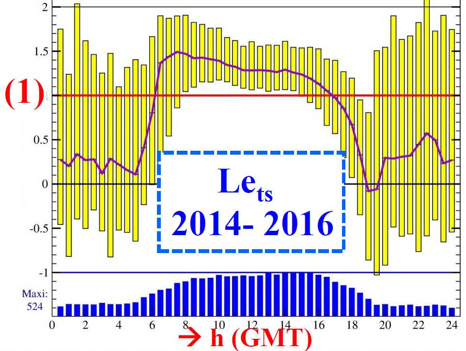
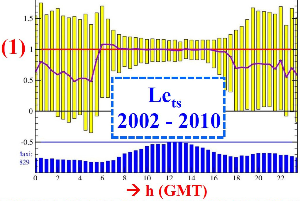
Figures 1 show that average yearly Lewis turbulent numbers computed with the the eddy-correlation method are significantly larger than unity in daytime, and are lower than at night. The significant level is more often reached for monthly averages Figures (not shown) and this diurnal cycle is also observed almost each days, with a maximum present just after sunrise. This maximum of is often larger than in June-August and if often smaller than in winter.
The observed diurnal cycle for may explain the previous disagreements in the articles of the 1970s: values close to may be observed in the late afternoon and values larger than unity in the early morning?
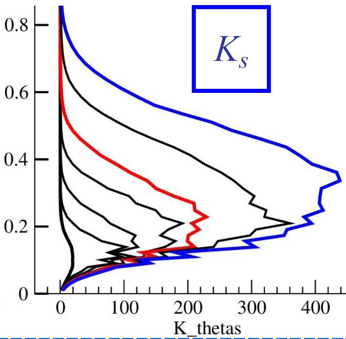
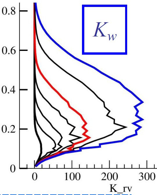

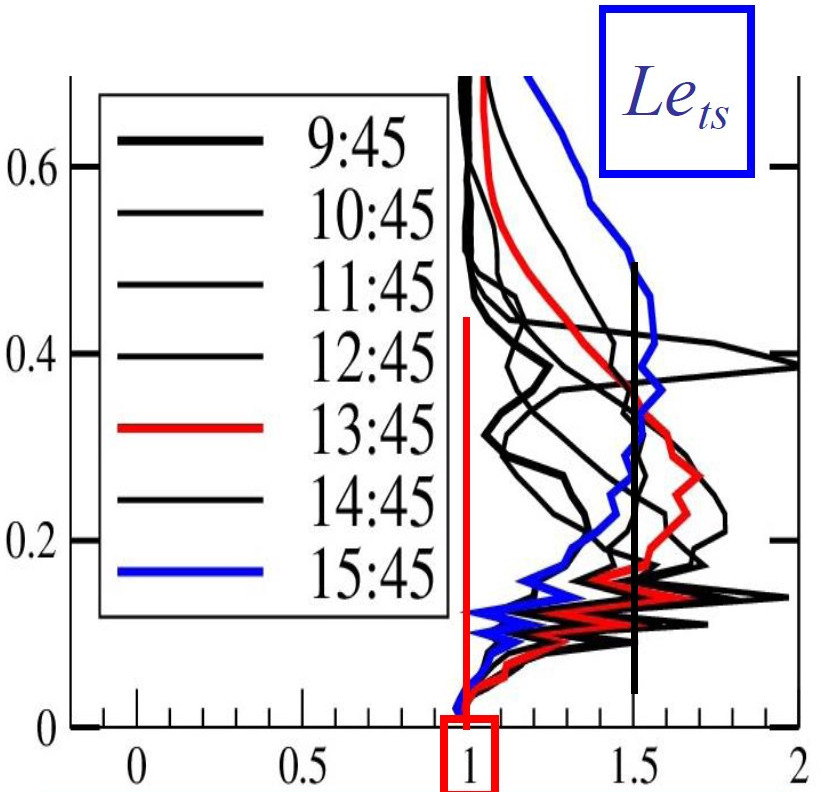
Figure 2 shows that the LES outputs for the IHOP case lead to robust computations of the new moist-air entropy exchange coefficient and of by means of the eddy-correlation method, whereas values of determined from the flux and the vertical gradient of is subject to infinite values (due to zero vertical gradient from about to m, depending on the hour) and to a counter-gradient region (due to the same signs of flux and vertical gradient above the level of infinite value).
The turbulent Lewis number is close to close to the surface on Figure 2, and then increases with altitude, reaching values above above the m height where the mass-flux starts to be active.
4 Conclusion
Values of the turbulent Lewis number significantly smaller or larger than are observed for the Météopole-Flux and the Cabauw masts, and simulated by a LES of the IHOP case. Consequently, it is necessary to revisit the equations of turbulence and to determined the values of several new constant coefficients (for the pressure and the second-order moment terms). These observations and simulations outputs will be used to compute these coefficients.
References
Betts AK. (1973). Non-precipitating cumulus convection and its parameterization. Q. J. R. Meteorol. Soc. 99 (419): 178–196.
Couvreux F. et al. (2005). Water-vapour variability within a convective boundary-layer assessed by large-eddy simulations and IHOP 2002 observations. Q. J. R. Meteorol. Soc. 131 (611): p.2665-2693. http://dx.doi.org/10.1256/qj.04.167
Hauf T. and Höller H. (1987). Entropy and potential temperature. J. Atmos. Sci., 44 (20): p.2887-2901.
Marquet P. (2011). Definition of a moist entropic potential temperature. Application to FIRE-I data flights. Q. J. R. Meteorol. Soc. 137 (656): p.768–791. http://arxiv.org/abs/1401.1097
Marquet P. (2015). An improved approximation for the moist-air entropy potential temperature . WGNE Blue-Book. http://arxiv.org/abs/1503.02287
Marquet P. (2016). The mixed-phase version of moist-air entropy. WGNE Blue-Book. http://arxiv.org/abs/1605.04382
Richardson L. F. (1919). Atmospheric stirring measured by precipitation. Proc. Roy. Soc. London (A). 96: p.9-18. https://ia600700.us.archive.org/32/items/philtrans07640837/07640837.pdf