Photon production spectrum above $T_{\rm c}$ with a lattice quark propagator

Abstract

The photon production rate from the deconfined medium is analyzed with the photon self-energy constructed from the quark propagator obtained by the numerical simulation on the quenched lattice for two values of temperature, $T=1.5T_{\rm c}$ and $3T_{\rm c}$, above the critical temperature $T_{\rm c}$. The photon self-energy is calculated by the Schwinger-Dyson equation with the lattice quark propagator and a vertex function determined so as to satisfy the Ward-Takahashi identity. The obtained photon production rate exhibits a similar behavior as the perturbative results at the energy of photons larger than $0.5$ GeV.

I Introduction

Photons are important observables in relativistic heavy-ion collisions FIRST ; Muller:2012zq . Because of its colorless nature, the mean free path of photons is longer than the size of the hot matter produced in heavy-ion collisions. Once photons are produced, therefore, they penetrate the hot medium without scatterings via the strong interaction. The experimental measurements of photon yield and anisotropic flow have been carried out actively Adare:2014fwh ; Adam:2015lda .

The experimental results show that the photon yield from heavy-ion collisions has an excess at lower transverse momentum regions Adare:2014fwh ; Adam:2015lda compared with the reference yield obtained by the superposition of proton-proton collisions. This result suggests the importance of the photon radiation from the hot medium. The other important observable is the photon anisotropic flow. The magnitude of the observed photon flows is almost the same as that of the medium Adare:2015lcd . The large anisotropic flow implies that photons are dominantly emitted from late stages in which the flow of the medium has been well developed. Phenomenological analyses of photon yield based on dynamical models have not succeeded in reproducing these experimental results simultaneously so far Paquet:2015lta ; Shen:2013cca . Photons are produced via several mechanisms during the time evolution of heavy-ion collisions. The discrepancy between the phenomenological analysis and experimental results suggests the importance of careful surveys of the production rates through these different production mechanisms. In the present study, among these mechanisms we focus on the photon radiation from the hot deconfined medium.

In the previous phenomenological analyses on the photon yield and flows Paquet:2015lta ; Shen:2013cca , the photon production rate calculated in perturbation theory Kapusta:1991qp ; Baier:1991em ; Arnold:2001ba ; Arnold:2001ms ; Ghiglieri:2013gia has been used for those from deconfined medium. On the other hand, the success of hydrodynamic models in describing the time evolution of the hot medium suggests that the deconfined medium is a strongly coupled system Hirano:2005wx ; Hirano:2005xf , in which a perturbative analysis would lose its validity. A non-perturbative analysis thus is desirable to evaluate the production rate from the deconfined medium. However, the direct analysis of the emission rate in lattice QCD numerical simulations is quite difficult, because this analysis requires an analysis of on-shell spectral functions.

In this paper, we analyze the photon production rate from the deconfined medium by partially using the lattice data in order to incorporate the non-perturbative effects in the analysis. The photon production rate is related to the photon self-energy in medium McLerran:1984ay ; Weldon:1990iw ; Gale:1990pn . From the Schwinger-Dyson equation (SDE), the full photon self-energy is constructed from the full quark propagator and the full photon-quark vertex. In Refs. Karsch:2007wc ; Karsch:2009tp ; Kaczmarek:2012mb , the quark propagator in the deconfined medium is analyzed on the quenched lattice in Landau gauge with a pole ansatz. We employ this lattice propagator as the full quark propagator in the SDE. A photon-quark vertex is constructed from the lattice quark propagator so as to satisfy the Ward-Takahashi identity. Our analysis thus respects gauge invariance. The same analysis has been applied to the calculation of the dilepton production rate at zero three-momentum in our previous study Kim:2015poa . The present study extends this analysis to nonzero momentum to calculate the photon production rate.

We analyze the photon production rate for two temperatures, $T=1.5T_{\rm c}$ and $3T_{\rm c}$, where $T_{\rm c}$ is the pseudo critical temperature. We show that the photon production is dominated by the pair annihilation and Landau damping of two quasi-particle, the normal and plasmino, modes. Although the pair annihilation cannot produce real photons in the perturbative analysis, in our formalism peculiar dispersion relations of quasi-particle modes in the lattice quark propagator allow the process. We find that the obtained photon production rate exhibits a similar behavior as the perturbative results both in the slope and the magnitude at the photon energy larger than $0.5$ GeV, although the photon production mechanism is completely different.

The outline of this paper is as follows. In the next section, we introduce the SDE for the photon self-energy, and discuss the construction of its components, the lattice quark propagator and a photon-quark vertex satisfying the Ward-Takahashi identity. In Sec. III, we calculate the photon self-energy with this setup with and without vertex correction. In Sec. IV, we show the numerical results on the photon production spectrum. The final section is devoted to a summary.

II Schwinger-Dyson equation for Photon Self-Energy

II.1 Schwinger-Dyson equation

The photon production rate from a static medium per unit time per unit volume is related to the retarded photon self-energy $\Pi_{\mu\nu}^{R}(\omega,\bm{q})$ as McLerran:1984ay ; Weldon:1990iw ; Gale:1990pn

$$\omega\frac{dN_{\gamma}}{d^{3}qd^{4}x}=-\frac{1}{(2\pi)^{3}}\frac{1}{{\rm e}^{\beta\omega}-1}{\rm Im}\Pi_{\mu}^{R,\mu}(\omega,\bm{q}),$$ (1)

with the inverse temperature $\beta=1/T$ and the four-momentum of photon $(\omega,\bm{q})$. This formula is correct at the leading order in electromagnetic interaction and all orders in strong interaction. The retarded photon self-energy is related to the imaginary-time self-energy $\Pi_{\mu\nu}(i\omega_{m},\bm{q})$ by the analytic continuation,

$$\Pi^{R}_{\mu\nu}(\omega,\bm{q})=\Pi_{\mu\nu}(i\omega_{m},\bm{q})|_{i\omega_{m}\rightarrow\omega+i\eta},$$ (2)

with the positive infinitesimal number $\eta$ and the Matsubara frequency for bosons $\omega_{m}=2\pi Tm$ with integer $m$. The imaginary-time full photon self-energy is given by the SDE in Matsubara formalism with the full quark propagator $S(P)$ and the full photon-quark vertex $\Gamma_{\mu}(P+Q,P)$ as

$$\Pi_{\mu\nu}(i\omega_{m},\bm{q})= -\sum_{f}e_{f}^{2}T\sum_{n}\int\frac{d^{3}p}{(2\pi)^{3}}$$

$${\rm Tr_{C}Tr_{D}}[S(P)\gamma_{\mu}S(P+Q)\Gamma_{\nu}(P+Q,P)],$$ (3)

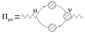
where $P_{\mu}=(i\nu_{n},\bm{p})$ and $Q_{\mu}=(i\omega_{m},\bm{q})$ are the four-momenta of quarks and photons, respectively, and $\nu_{n}=(2n+1)\pi T$ with integer $n$ is the Matsubara frequency for fermions. $e_{f}$ is the electric charge of quarks with the index $f$ representing the quark flavor. The color, flavor, and Dirac indices of $S(P)$ are suppressed for notational simplicity, and ${\rm Tr_{C}}$ and ${\rm Tr_{D}}$ represent the trace over the color and Dirac indices, respectively. In covariant gauges, the off-diagonal elements of the quark propagator in color space vanish. As a result, the trace over the color indices gives a factor three in Eq. (3). In Fig. 1, we show the diagrammatic representation of Eq. (3). The shaded circles mean the full propagator and vertex function. In the following, we consider the two-flavor QCD with degenerate $u$ and $d$ quarks, in which $\sum_{f}e_{f}^{2}=5e^{2}/9$.

Figure 1: Diagrammatic representation of the Schwinger-Dyson equation for the full photon self-energy, Eq. (3). The shaded circles mean the full quark propagator and the full photon-quark vertex.

II.2 Lattice quark propagator and spectral function

In the present study, we employ the quark propagator obtained in the lattice numerical simulation in Ref. Karsch:2007wc ; Karsch:2009tp ; Kaczmarek:2012mb for the full quark propagator in Eq. (3). This approach was used in our previous study for the analysis of the dilepton production rate at zero three-momentum Kim:2015poa . In this subsection, we give a brief review on the general property of the quark propagator and discuss the implementation of the results in Ref. Kaczmarek:2012mb in our analysis.

The imaginary-time quark propagator for momentum $\bm{p}$ is defined by

$$S_{\mu\nu}(\tau,\bm{p})=\int d^{3}x{\rm e}^{-i\bm{p}\cdot\bm{x}}\langle\psi_{\mu}(\tau,\bm{x})\bar{\psi}_{\nu}(0,\bm{0})\rangle,$$ (4)

where $\psi_{\mu}(\tau,\bm{x})$ is the quark field with the Dirac index $\mu$, and $\tau$ is the imaginary time restricted to the interval $0\leq\tau<\beta$. We show the Dirac indices of quark fields explicitly for a moment. The Fourier transform of Eq. (4) is given by

$$S_{\mu\nu}(i\nu_{n},\bm{p})=\int_{0}^{\beta}d\tau{\rm e}^{i\nu_{n}\tau}S_{\mu\nu}(\tau,\bm{p}).$$ (5)

Equation (5) is rewritten with the quark spectral function $\rho_{\mu\nu}(\nu,\bm{p})$ as

$$S_{\mu\nu}(i\nu_{n},\bm{p})=-\int_{-\infty}^{\infty}d\nu^{\prime}\frac{\rho_{\mu\nu}(\nu^{\prime},\bm{p})}{\nu^{\prime}-i\nu_{n}}.$$ (6)

From Eqs. (5) and (6), the spectral function is related to Eq. (4) as

$$S_{\mu\nu}\left(\tau,\bm{p}\right)=\int_{-\infty}^{\infty}d\nu\frac{\mbox{e}^{\left(1/2-\tau/\beta\right)\beta\nu}}{\mbox{e}^{\beta\nu/2}+\mbox{e}^{-\beta\nu/2}}\rho_{\mu\nu}\left(\nu,\bm{p}\right).$$ (7)

When chiral symmetry is restored, the quark propagator anticommutes with $\gamma_{5}$. In this case, one can decompose the quark spectral function with the projection operators $\Lambda_{\pm}\left(\bm{p}\right)=\left(1\pm\gamma_{0}\hat{\bm{p}}\cdot\bm{\gamma}\right)/2$ as

$$\rho(\nu,\bm{p})=\rho_{+}(\nu,p)\Lambda_{+}(\bm{p})\gamma_{0}+\rho_{-}(\nu,p)\Lambda_{-}(\bm{p})\gamma_{0},$$ (8)

with $p=|\bm{p}|$, $\hat{\bm{p}}=\bm{p}/p$, and

$$\rho_{\pm}(\nu,p)=\frac{1}{2}\mbox{Tr}_{\rm D}[\rho(\nu,\bm{p})\gamma_{0}\Lambda_{\pm}(\bm{p})].$$ (9)

From the anticommutation relation of $\psi$ and $\bar{\psi}$, one can derive the sum rule

$$\int_{-\infty}^{\infty}d\nu\rho_{\pm}(\nu,p)=1.$$ (10)

Using the charge conjugation symmetry of thermal ensemble, one can also show that $\rho_{\pm}$ satisfy Kaczmarek:2012mb

$$\rho_{\pm}(\nu,p)=\rho_{\mp}(-\nu,p).$$ (11)

In Refs. Karsch:2007wc ; Karsch:2009tp ; Kaczmarek:2012mb , the imaginary-time quark propagator Eq. (4) is evaluated on the lattice in Landau gauge with the quenched approximation. On the lattice the quark propagator is measured for discrete imaginary times. To obtain the real time information, one has to deduce the spectral function from the discrete information. In Refs. Karsch:2007wc ; Karsch:2009tp ; Kaczmarek:2012mb , the spectral function $\rho_{\pm}(\nu,p)$ is analyzed with the two-pole ansatz,

$$\rho_{+}(\nu,p)=Z_{+}(p)\delta\left(\nu-\nu_{+}(p)\right)+Z_{-}(p)\delta\left(\nu+\nu_{-}(p)\right),$$ (12)

where $Z_{\pm}(p)$ and $\nu_{\pm}(p)$ are the residues and positions of the poles, respectively, which are determined by fitting to the lattice propagator for each $p$.

Comments on the two-pole ansatz Eq. (12) are in order. First, two particle-like states $\nu_{+}(p)$ and $\nu_{-}(p)$ in Eq. (12) correspond to the normal and plasmino modes, respectively, which appear in the quark propagator in the hard thermal loop approximation LeBellac . In fact, the analyses in Refs. Karsch:2007wc ; Karsch:2009tp ; Kaczmarek:2012mb suggest that these modes behave like the normal and plasmino modes as functions of momentum $p$ and bare quark mass $m_{0}$. For example, for large $p$ and $m_{0}$ the residue of the plasmino mode $Z_{-}(p)$ becomes small and the propagator approaches the one of the free quark. Second, the restoration of chiral symmetry for massless quarks above the pseudo-critical temperature $T_{\rm c}$ is confirmed explicitly on the lattice by measuring the scalar term of the quark propagator Karsch:2009tp ; Kaczmarek:2012mb . Third, in Refs. Karsch:2009tp ; Kaczmarek:2012mb various fitting ansätze have been tested besides the two-pole ansatz Eq. (12), such as an ansatz which allows non-zero widths of the poles in Eq. (12). However, it was turned out that fitting with widths does not improve $\chi^{2}$, as the minimum of the $\chi^{2}$ is at vanishing widths. From these results, we suppose that the existence of sharp quasi-particle states in the quark spectral function is supported from the lattice analysis. Fourth, the quark propagator depends on the gauge in general, while the analyses on the lattice have been performed in Landau gauge. We, however, note that the positions of poles in the quark propagator are independent of the gauge Rebhan:1993az .

Figure 2: Open symbols show the momentum dependence of the parameters $\nu_{+}(p)$, $\nu_{-}(p)$, and $Z_{-}(p)/(Z_{+}(p)+Z_{-}(p))$ obtained on the lattice in Ref. Kaczmarek:2012mb . The solid lines represent their interpolation obtained by the cubic spline method. The dashed line in the upper panel represents the light cone.

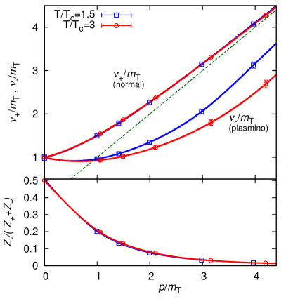
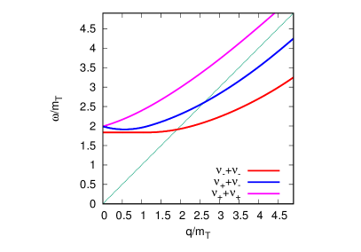
In Fig. 2, we show the $p$ dependences of the fitting parameters in Eq. (12) obtained in Ref. Kaczmarek:2012mb for $T=1.5T_{\rm c}$ and $3T_{\rm c}$. The upper panel shows the dispersions relation $\nu_{+}(p)$ and $\nu_{-}(p)$, while the lower panel shows the relative strength of the residue of the plasmino mode $Z_{-}(p)/(Z_{+}(p)+Z_{-}(p))$. These analyses are performed on lattices with volume $128^{3}\times 16$, where both the lattice spacing and finite volume effects are found to be small Kaczmarek:2012mb . The two axes in the upper panel are normalized by the thermal mass $m_{\rm T}$ defined by the energy of the quasi-particle excitations at $p=0$ as $m_{\rm T}=(\nu_{+}(0)+\nu_{-}(0))/2$. After the extrapolation to infinite volume, $m_{\rm T}/T$ is estimated as 0.768(11) and 0.725(14) at $T=1.5T_{\rm c}$ and $3T_{\rm c}$, respectively Kaczmarek:2012mb .

Although the lattice data are available only for discrete values of $p$ because of the periodic boundary condition, one needs the quark propagator as a continuous function of $p$ to solve Eq. (3). To obtain the fitting parameters as continuous functions of $p$, we perform the interpolation of the lattice data by the cubic spline method. From Eq. (11), one can show that $d\nu_{+}(p)/dp=-d\nu_{-}(p)/dp$, $d^{2}\nu_{+}(p)/dp^{2}=d^{2}\nu_{-}(p)/dp^{2}$, and $Z_{+}(p)=Z_{-}(p)$ at $p=0$ Karsch:2009tp ; Kaczmarek:2012mb . These properties are taken into account in the interpolation. The lattice data are available only in the momentum range $p/T\lesssim 4.7$, and we need the extrapolation to higher momentum. We extrapolate the parameters using an exponentially damping form for $Z_{-}(p)/(Z_{+}(p)+Z_{-}(p))$,

$$Z_{-}(p)/(Z_{+}(p)+Z_{-}(p))=R{\rm e}^{-\alpha p},$$ (13)

and

$$\nu_{\pm}(p)=p+\beta^{\pm}_{1}{\rm e}^{-\beta^{\pm}_{2}p},$$ (14)

for $\nu_{\pm}(p)$, which approaches the light cone exponentially for large $p$. The parameters $R$, $\alpha$, and $\beta^{\pm}_{i}$ are determined in the cubic spline analysis. The $p$ dependence of each parameter determined in this way is shown by the solid lines in Fig. 2. We tested another extrapolation form, $\nu_{\pm}(p)=p+\beta^{\prime\pm}_{1}/p+\beta^{\prime\pm}_{2}/p^{2}+\cdots$, but found that the dispersion relations hardly change. Finally, we set

$$Z_{+}(p)+Z_{-}(p)=1$$ (15)

to satisfy the sum rule Eq. (10).

We note that the slope of the plasmino dispersion relation exceeds unity for $p\gtrsim 3m_{\rm T}$ and is acausal. This unphysical behavior may come from an artifact of the lattice simulation and/or the ansatz for the spectral function. This acausal behavior gives rise to the Cherenkov radiation, as we will see in later sections. However, as we show explicitly in Sec. IV, the residue of the plasmino mode is small, $Z_{-}(p)<0.05$, in this momentum range and the contribution of the Cherenkov radiation to our final result is negligibly small except for the low energy region $\omega\lesssim 0.1$ GeV.

Using Eqs. (6), (8), and (12), the quark propagator is given by

$$S(i\nu_{n},\bm{p}) =S_{+}(i\nu_{n},p)\Lambda_{+}(\bm{p})\gamma_{0}+S_{-}(i\nu_{n},p)\Lambda_{-}(\bm{p})\gamma_{0},$$

$$=\sum_{s=\pm 1}S_{s}(i\nu_{n},p)\Lambda_{s}(\bm{p})\gamma_{0},$$ (16)

with

$$S_{s}(i\nu_{n},p)=\frac{Z_{+}(p)}{i\nu_{n}-s\nu_{+}(p)}+\frac{Z_{-}(p)}{i\nu_{n}+s\nu_{-}(p)},$$ (17)

where we define $S_{\pm 1}(P)=S_{\pm}(P)$ and $\Lambda_{\pm 1}(\bm{p})=\Lambda_{\pm}(\bm{p})$ for notational simplicity. Correspondingly, the inverse quark propagator is given by

$$S^{-1}(i\nu_{n},\bm{p})=\sum_{s=\pm 1}S_{s}^{-1}(i\nu_{n},p)\gamma_{0}\Lambda_{s}(\bm{p}),$$ (18)

with

$$S_{s}^{-1}(i\nu_{n},p)=\frac{(i\nu_{n}-s\nu_{+}(p))(i\nu_{n}+s\nu_{-}(p))}{i\nu_{n}+sV(p)},$$ (19)

and $V(p)=Z_{+}(p)\nu_{-}(p)-Z_{-}(p)\nu_{+}(p)$. Note that the inverse propagator has poles at $i\nu_{n}=\pm V(p)$. These poles inevitably appear in the multipole ansatz, because the propagator $S_{s}(\omega,p)$ after the analytic continuation to real time has one zero point in the range of $\omega$ surrounded by two poles. We will see that the poles at $i\nu_{n}=\pm V(p)$ give rise to additional photon production mechanism that we call “anomalous” productions.

II.3 Photon-Quark Vertex

To solve the SDE, Eq. (3), one needs the full photon-quark vertex $\Gamma_{\mu}(P+Q,P)$ besides the full quark propagator. The vertex $\Gamma_{\mu}(P+Q,P)$ must satisfy the Ward-Takahashi identity (WTI)

$$Q^{\mu}\Gamma_{\mu}(P+Q,P)=S^{-1}(P+Q)-S^{-1}(P).$$ (20)

One, however, cannot determine the four components of the vertex uniquely from this constraint. In the present study, as the full vertex satisfying the WTI, we choose the following simple representation:

$$\Gamma_{0}(i\omega_{m}+i\nu_{n},\bm{p}+\bm{q};i\nu_{n},\bm{p})$$

$$=\frac{1}{2i\omega_{m}}\left[S^{-1}(i\omega_{m}+i\nu_{n},\bm{p}+\bm{q})-S^{-1}(i\nu_{n},\bm{p}+\bm{q})\right.$$

$$~{}~{}~{}\left.+S^{-1}(i\omega_{m}+i\nu_{n},\bm{p})-S^{-1}(i\nu_{n},\bm{p})\right],$$ (21)

$$\Gamma_{i}(i\omega_{m}+i\nu_{n},\bm{p}+\bm{q};i\nu_{n},\bm{p})$$

$$=\gamma_{i}-\frac{q_{i}}{2q^{2}}\left[S^{-1}(i\omega_{m}+i\nu_{n},\bm{p}+\bm{q})+S^{-1}(i\nu_{n},\bm{p}+\bm{q})\right.$$

$$~{}~{}~{}\left.-S^{-1}(i\omega_{m}+i\nu_{n},\bm{p})-S^{-1}(i\nu_{n},\bm{p})\right]-\frac{q_{i}(\bm{q}\cdot\bm{\gamma})}{q^{2}}.$$ (22)

One can easily check that Eqs. (21) and (22) satisfy the WTI Eq. (20). In this choice, we construct the vertex so that $\Gamma_{\mu}$ becomes the bare vertex $\gamma_{\mu}$ when the free quark propagator $S^{-1}(P)=\not p$ is substituted. Although our vertex Eqs. (21) and (22) is not the unique choice Ball:1980ay , we emphasize that our analysis with Eqs. (21) and (22) satisfies the gauge invariance required by the WTI.

III Photon Production Rate

Next, we construct the photon self-energy Eq. (3) from the lattice quark propagator and the gauge invariant photon-quark vertex obtained in the previous section. In this section, we analyze the photon self-energy for two cases. First, we calculate the photon production rate with the lattice quark propagator but with the bare vertex in Sec. III.1. This result will help us understand the effect of the vertex correction. Then, we perform the full analysis in Sec. III.2.

III.1 Photon Production Rate without Vertex Correction

In this subsection, we calculate the photon self-energy without the vertex correction with $\Gamma_{\mu}=\gamma_{\mu}$. The photon self-energy in this case is given by

$$\Pi_{\mu\nu}(i\omega_{m},\bm{q})= -\frac{5e^{2}}{3}T\sum_{n}\int\frac{d^{3}p}{(2\pi)^{3}}$$

$${\rm Tr_{D}}[S(i\nu_{n},\bm{p})\gamma_{\mu}S(i\omega_{m}+i\nu_{n},\bm{p}+\bm{q})\gamma_{\mu}].$$ (23)

By substituting the decomposition Eq. (16) into Eq. (23), one obtains

$$\Pi_{\mu\mu}(i\omega_{m},\bm{q})$$

$$=-\frac{5e^{2}}{3}T\sum_{n}\int\frac{d^{3}p}{(2\pi)^{3}}\sum_{s,t=\pm 1}S_{s}(i\nu_{n},p)S_{t}(i\omega_{m}+i\nu_{n},p)$$

$$\qquad{\rm Tr_{D}}[\Lambda_{s}(\bm{p})\gamma_{0}\gamma_{\mu}\Lambda_{t}(\bm{p}+\bm{q})\gamma_{0}\gamma_{\mu}]$$ (24)

$$=-\frac{5e^{2}}{12\pi^{2}q}T\sum_{n}\sum_{s,t=\pm 1}\int_{R}dp_{1}dp_{2}st[(sp_{1}-tp_{2})^{2}-q^{2}]$$

$$\qquad S_{s}(i\nu_{n},p_{1})S_{t}(i\omega_{m}+i\nu_{n},p_{2}),$$ (25)

with

$$p_{1}=|\bm{p}|,\quad p_{2}=|\bm{p}+\bm{q}|$$ (26)

being the momenta of the quarks, and $q=|\bm{q}|$, and we used ${\rm Tr_{D}}[\Lambda_{s}(\bm{p})\gamma_{0}\gamma_{\mu}\Lambda_{t}(\bm{p}+\bm{q})\gamma_{0}\gamma_{\mu}]=st[(sp_{1}-tp_{2})^{2}-q^{2}]$. In Eq. (25), we changed the three-momentum integral as

$$\int\frac{d^{3}p}{(2\pi)^{3}}=\int_{R}\frac{dp_{1}dp_{2}}{(2\pi)^{2}}\frac{p_{1}p_{2}}{q},$$ (27)

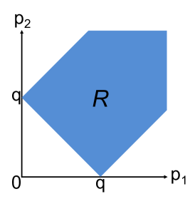
where the integral is carried out in the region $R$, which is surrounded by the lines $p_{1}+p_{2}=q$ and $p_{1}-p_{2}=\pm q$ as shown in Fig. 3. The region $R$ is defined by the $p_{1}$ and $p_{2}$ which can satisfy $|\bm{p}_{2}-\bm{p}_{1}|=|\bm{q}|$.

Figure 3: Integral region $R$ in Eq. (27).

Taking the analytic continuation $i\omega_{m}\to\omega+i\eta$ of Eq. (25) and the imaginary part, one obtains the imaginary part of the retarded self-energy,

$${\rm Im}\Pi_{\mu}^{R,\mu}(\omega,\bm{q})= \frac{5e^{2}}{12\pi q}\sum_{\begin{subarray}{c}s,t,\eta_{1},\eta_{2}\\ =\pm 1\end{subarray}}\int_{R}dp_{1}dp_{2}Z_{\eta_{1}}(p_{1})Z_{\eta_{2}}(p_{2})$$

$$st[(sp_{1}-tp_{2})^{2}-q^{2}]$$

$$[f(s\eta_{1}\nu_{\eta_{1}}(p_{1}))-f(t\eta_{2}\nu_{\eta_{2}}(p_{2}))]$$

$$\delta(\omega+s\eta_{1}\nu_{\eta_{1}}(p_{1})-t\eta_{2}\nu_{\eta_{2}}(p_{2})),$$ (28)

with $\nu_{\pm 1}(p)=\nu_{\pm}(p)$ and the Fermi distribution function $f(E)=1/[{\rm e}^{\beta E}+1]$.

Owing to the $\delta$-function, the momentum integral in Eq. (28) is reduced to the one-dimensional one. In Fig. 4, we show an example of the path determined by the $\delta$-function by the red line for $\omega=|\bm{q}|=5m_{\rm T}$ and $s=t=-\eta_{1}=\eta_{2}=-1$ at $T=1.5T_{\rm c}$; the line in this case satisfies $\nu_{+}(p_{1})+\nu_{-}(p_{2})=5m_{\rm T}$. In our numerical analysis, after determining the line in $R$ numerically we carry out the line integral.

Figure 4: An example of the path of line integral in Eq. (28) in the $p_{1}$–$p_{2}$ plane. The red line shows the line constrained by the $\delta$-function for $\omega=|\bm{q}|=5m_{\rm T}$ and $s=t=-\eta_{1}=\eta_{2}=-1$ at $T=1.5T_{\rm c}$.

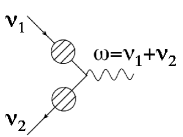
Equation (28) consists of 16 terms with $s,t,\eta_{1},\eta_{2}=\pm 1$. These terms are interpreted as the photon production rates from the decay and scatterings of two quasi-quarks as follows. First, the $\delta$-function in each term expresses the energy conservation, and the residues $Z_{\pm}$ represent those of the corresponding quasi-particles. Next, the thermal factor $f(s\eta_{1}\nu_{\eta_{1}}(p_{1}))-f(t\eta_{2}\nu_{\eta_{2}}(p_{2}))$ is transformed as $-[1-f(\nu_{1})-f(\nu_{2})]$ or $f(\nu_{1})-f(\nu_{2})$ for a given set of $(s,t,\eta_{1},\eta_{2})$ with $\nu_{1}=\nu_{\pm}(p_{1})$ and $\nu_{2}=\nu_{\pm}(p_{2})$. When the thermal factor becomes $-[1-f(\nu_{1})-f(\nu_{2})]$, this factor can be rewritten as

$$-[1-f(\nu_{1})-f(\nu_{2})]$$

$$=f(\nu_{1})f(\nu_{2})-(1-f(\nu_{1}))(1-f(\nu_{2})).$$ (29)

Because this is the difference between the products of thermal distributions and Pauli blocking effects, this term is interpreted as the difference of the photon emission from the pair annihilation of quasi-quarks shown in Fig. 5(a) and the photon absorption mediated by its inverse process. Similarly, we have

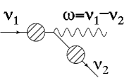
$$f(\nu_{1})-f(\nu_{2})=f(\nu_{1})(1-f(\nu_{2}))-(1-f(\nu_{1}))f(\nu_{2}).$$ (30)

The photon emission and absorption of this term is diagrammatically represented as in Fig. 5(b), which is called the Landau damping Landau:1946jc .

(a) Pair annihilation

(b) Landau damping

Figure 5: Photon production processes with two quasi-quarks. Shaded circles represent the lattice quark propagator having two quasi-particle modes.

In the perturbative calculation, the pair annihilation with two quasi-particles cannot produce a real photon Kapusta:1991qp ; Baier:1991em ; Arnold:2001ba ; Arnold:2001ms . This is because the quasi-particle states are in the time like region and these processes cannot fulfill the on-shell condition in the processes in Fig. 5. On the other hand, as in Fig. 2 the plasmino mode in the lattice quark propagator enters space-like region. Because of this behavior, it is possible that the pair annihilation produces a real photon directly. This is the most remarkable difference of our analysis from the perturbative one.

Note that we are interested in the photon production rate, while ${\rm Im}\Pi^{R,\mu}_{\mu}$ represents the difference of the production and absorption rates as shown above. To obtain the former, as in Eq. (1) one multiplies the Bose distribution function $1/[{\rm e}^{\beta\omega}-1]$ to ${\rm Im}\Pi_{\mu}^{R,\mu}(\omega,\bm{q})$. Indeed, we have

$$\frac{1}{{\rm e}^{\beta\omega}-1}[1-f(\nu_{1})-f(\nu_{2})]\delta(\omega-\nu_{1}-\nu_{2})$$

$$=f(\nu_{1})f(\nu_{2})\delta(\omega-\nu_{1}-\nu_{2}).$$ (31)

III.2 Full Photon Production Rate

Now, we consider the photon self-energy with the full vertex Eqs. (21) and (22).

First, we calculate ${\rm Im}\Pi_{00}(\omega,\bm{q})$. The trace in Eq. (3) is calculated to be

$${\rm Tr_{D}}[S(P_{1})\gamma_{0}S(P_{2})\Gamma_{0}(P_{2},P_{1})]$$

$$=\sum_{s,t=\pm 1}\frac{1}{2i\omega_{m}}{\rm Tr_{D}}[\Lambda_{s}(p_{1})\Lambda_{t}(p_{2})]\left[S_{s}(i\nu_{n},p_{1})\left[1-\frac{S_{t}(i\omega_{m}+i\nu_{n},p_{2})}{S_{t}(i\nu_{n},p_{2})}\right]-S_{t}(i\omega_{m}+i\nu_{n},p_{2})\left[1-\frac{S_{s}(i\nu_{n},p_{1})}{S_{s}(i\omega_{m}+i\nu_{n},p_{1})}\right]\right]$$

$$=\sum_{s,t,\epsilon=\pm 1}\frac{1}{2}{\rm Tr_{D}}[\Lambda_{s}(p_{1})\Lambda_{t}(p_{2})]\left[S_{s}(i\nu_{n},p_{1})\frac{Z_{\epsilon}(p_{2})(i\nu_{n}+t\epsilon\nu_{\bar{\epsilon}}(p_{2}))}{(i\omega_{m}+i\nu_{n}-\epsilon t\nu_{\epsilon}(p_{2}))(i\nu_{n}+tV(p_{2}))}\right.$$

$$~{}~{}~{}~{}\left.+S_{t}(i\omega_{m}+i\nu_{n},p_{2})\frac{Z_{\epsilon}(p_{1})(i\omega_{m}+i\nu_{n}+s\epsilon\nu_{\bar{\epsilon}}(p_{1}))}{(i\nu_{n}-\epsilon s\nu_{\epsilon}(p_{1}))(i\omega_{m}+i\nu_{n}+sV(p_{1}))}\right],$$ (32)

with $\nu_{\bar{\epsilon}}=\nu_{-\epsilon}$, where in the first and second equalities we used, respectively, the decomposition Eq. (16) and the two-pole form Eq. (17). Using $V(p)+\eta\nu_{\eta}(p)=\eta Z_{\eta}(p)\bar{\nu}(p)$ and $V(p)+\bar{\eta}\nu_{\bar{\eta}}(p)=\bar{\eta}Z_{\bar{\eta}}(p)\bar{\nu}(p)$ with $\bar{\nu}(p)=\nu_{+}(p)+\nu_{-}(p)$, $\Pi_{00}(i\omega_{m},\bm{q})$ is given by

$$\Pi_{00}(i\omega_{m},\bm{q})=-\frac{5e^{2}}{12(2\pi)^{2}q}\sum_{\begin{subarray}{c}s,t,\eta_{1},\eta_{2}\\ =\pm 1\end{subarray}}\int_{R}dp_{1}dp_{2}st[(sp_{1}+tp_{2})^{2}-q^{2}]Z_{\eta_{1}}(p_{1})Z_{\eta_{2}}(p_{2})$$

$$~{}~{}~{}~{}\left[\left(2+\frac{t\eta_{2}Z_{\bar{\eta}_{2}}(p_{2})\bar{\nu}(p_{2})}{s\eta_{1}\nu_{\eta_{1}}(p_{1})+tV(p_{2})}+\frac{s\eta_{1}Z_{\bar{\eta}_{1}}(p_{1})\bar{\nu}(p_{1})}{t\eta_{2}\nu_{\eta_{2}}(p_{2})+sV(p_{1})}\right)\right.\frac{f(s\eta_{1}\nu_{\eta_{1}}(p_{1}))-f(t\eta_{2}\nu_{\eta_{2}}(p_{2}))}{i\omega_{m}+s\eta_{1}\nu_{\eta_{1}}(p_{1})-t\eta_{2}\nu_{\eta_{2}}(p_{2})}$$

$$~{}~{}~{}~{}\left.-\frac{t\eta_{2}Z_{\bar{\eta}_{2}}(p_{2})\bar{\nu}(p_{2})}{s\eta_{1}\nu_{\eta_{1}}(p_{1})+tV(p_{2})}\cdot\frac{f(-tV(p_{2}))-f(t\eta_{2}\nu_{\eta_{2}}(p_{2}))}{i\omega_{m}-tV(p_{2})-t\eta_{2}\nu_{\eta_{2}}(p_{2})}-\frac{s\eta_{1}Z_{\bar{\eta}_{1}}(p_{1})\bar{\nu}(p_{1})}{t\eta_{2}\nu_{\eta_{2}}(p_{2})+sV(p_{1})}\cdot\frac{f(s\eta_{1}\nu_{\eta_{1}}(p_{1}))-f(-sV(p_{1}))}{i\omega_{m}+s\eta_{1}\nu_{\eta_{1}}(p_{1})+sV(p_{1})}\right].$$ (33)

Performing the analytic continuation and taking the imaginary part, one obtains ${\rm Im}\Pi_{00}^{R}(\omega,\bm{q})$ as

$${\rm Im}\Pi_{00}^{R}(\omega,\bm{q})=\frac{5\alpha}{12q}\sum_{\begin{subarray}{c}s,t,\eta_{1},\eta_{2}\\ =\pm 1\end{subarray}}\int_{R}dp_{1}dp_{2}st[(sp_{1}+tp_{2})^{2}-q^{2}]Z_{\eta_{1}}(p_{1})Z_{\eta_{2}}(p_{2})$$

$$~{}~{}~{}~{}\left[\left(2+\frac{t\eta_{2}Z_{\bar{\eta}_{2}}(p_{2})\bar{\nu}(p_{2})}{s\eta_{1}\nu_{\eta_{1}}(p_{1})+tV(p_{2})}+\frac{s\eta_{1}Z_{\bar{\eta}_{1}}(p_{1})\bar{\nu}(p_{1})}{t\eta_{2}\nu_{\eta_{2}}(p_{2})+sV(p_{1})}\right)\right.[f(s\eta_{1}\nu_{\eta_{1}}(p_{1}))-f(t\eta_{2}\nu_{\eta_{2}}(p_{2}))]\delta(\omega+s\eta_{1}\nu_{\eta_{1}}(p_{1})-t\eta_{2}\nu_{\eta_{2}}(p_{2}))$$

$$~{}~{}~{}~{}-\frac{t\eta_{2}Z_{\bar{\eta}_{2}}(p_{2})\bar{\nu}(p_{2})}{s\eta_{1}\nu_{\eta_{1}}(p_{1})+tV(p_{2})}[f(-tV(p_{2}))-f(t\eta_{2}\nu_{\eta_{2}}(p_{2}))]\delta(\omega-tV(p_{2})-t\eta_{2}\nu_{\eta_{2}}(p_{2}))$$

$$~{}~{}~{}~{}\left.-\frac{s\eta_{1}Z_{\bar{\eta}_{1}}(p_{1})\bar{\nu}(p_{1})}{t\eta_{2}\nu_{\eta_{2}}(p_{2})+sV(p_{1})}[f(s\eta_{1}\nu_{\eta_{1}}(p_{1}))-f(-sV(p_{1}))]\delta(\omega+s\eta_{1}\nu_{\eta_{1}}(p_{1})+sV(p_{1}))\right].$$ (34)

Next, we analyze $\sum_{i}{\rm Im}\Pi_{ii}^{R}$. We decompose $\sum_{i}\Pi_{ii}$ into three parts, $\Pi_{ii}(Q)=\sum_{j=1}^{3}\Pi_{ii}^{(j)}(Q)$, where

$$\Pi_{ii}^{(j)}(Q)=-\frac{5}{3}T\sum_{n}\int\frac{d^{3}p}{(2\pi)^{3}}{\rm Tr_{D}}[S(P)\gamma_{i}S(P+Q)\Gamma_{i}^{(j)}],$$ (35)

with

$$\Gamma_{i}^{(1)} =\gamma_{i},$$ (36)

$$\Gamma_{i}^{(2)} =-\frac{q_{i}}{2q^{2}}\left[S^{-1}(i\omega_{m}+i\nu_{n},\bm{p}+\bm{q})+S^{-1}(i\nu_{n},\bm{p}+\bm{q})\right.$$

$$~{}~{}~{}\left.-S^{-1}(i\omega_{m}+i\nu_{n},\bm{p})-S^{-1}(i\nu_{n},\bm{p})\right],$$ (37)

$$\Gamma_{i}^{(3)} =-\frac{q_{i}(\bm{q}\cdot\bm{\gamma})}{q^{2}}.$$ (38)

The analysis of $\sum_{i}{\rm Im}\Pi_{ii}^{(1),R}(\omega,\bm{q})$ can be carried out in the same way as in Sec. III.1. The result is given by

$$\sum_{i=1}^{3}{\rm Im}\Pi_{ii}^{(1),R}(\omega,\bm{q})= -\frac{5\alpha}{3q}\sum_{\begin{subarray}{c}s,t,\eta_{1},\eta_{2}\\ =\pm 1\end{subarray}}\int_{R}dp_{1}dp_{2}Z_{\eta_{1}}(p_{1})Z_{\eta_{2}}(p_{2})\left[\frac{st[(sp_{1}+tp_{2})^{2}-q^{2}]}{2}-4p_{1}p_{2}\right]$$

$$[f(s\eta_{1}\nu_{\eta_{1}}(p_{1}))-f(t\eta_{2}\nu_{\eta_{2}}(p_{2}))]\delta(\omega+s\eta_{1}\nu_{\eta_{1}}(p_{1})-t\eta_{2}\nu_{\eta_{2}}(p_{2})).$$ (39)

Next, we consider $\sum_{i}{\rm Im}\Pi_{ii}^{(2),R}(\omega,\bm{q})$. The trace of this term is calculated to be

$${\rm Tr_{D}}[S(P)\gamma_{i}S(P+Q)[S^{-1}(i\omega_{m}+i\nu_{n},\bm{p}+\bm{q})+S^{-1}(i\omega_{m},\bm{p}+\bm{q})-S^{-1}(i\omega_{m}+i\nu_{n},\bm{p})-S^{-1}(i\nu_{n},\bm{p})]]$$

$$=\sum_{s,t}{\rm Tr_{D}}[\Lambda_{s}(\bm{p})\gamma_{0}\gamma_{i}\Lambda_{t}(\bm{p}+\bm{q})]\left[S_{s}(i\nu_{n},p_{1})\left[1+\frac{S_{t}(i\omega_{m}+i\nu_{n},p_{2})}{S_{t}(i\nu_{n},p_{2})}\right]-S_{t}(i\omega_{m}+i\nu_{n},p_{2})\left[1+\frac{S_{s}(i\nu_{n},p_{1})}{S_{s}(i\omega_{m}+i\nu_{n},p_{1})}\right]\right]$$

$$\to\sum_{s,t}{\rm Tr_{D}}[\Lambda_{s}(\bm{p})\gamma_{0}\gamma_{i}\Lambda_{t}(\bm{p}+\bm{q})]\left[S_{s}(i\nu_{n},p_{1})\left[\frac{S_{t}(i\omega_{m}+i\nu_{n},p_{2})}{S_{t}(i\nu_{n},p_{2})}-1\right]-S_{t}(i\omega_{m}+i\nu_{n},p_{2})\left[\frac{S_{s}(i\nu_{n},p_{1})}{S_{s}(i\omega_{m}+i\nu_{n},p_{1})}-1\right]\right],$$ (40)

where in the final step we used the fact that $S_{s}(i\nu_{n},p_{1})-S_{t}(i\omega_{m}+i\nu_{n},p_{2})$ vanishes after this term is integrated out and summed over $s$ and $t$ in Eq. (35). Using Eq. (40) one finds that $\sum_{i}{\rm Im}\Pi_{ii}^{(2),R}(\omega,\bm{q})$ has the same form as in Eq. (34) but the factor $\omega(tp_{2}-sp_{1})/q^{2}$ is applied to the integrand.

The last piece $\sum_{i}{\rm Im}\Pi_{ii}^{(3),R}(\omega,\bm{q})$ is calculated as

$$\sum_{i}{\rm Im}\Pi_{ii}^{(3),R}= \frac{5\alpha}{3q}\sum_{\begin{subarray}{c}s,t,\eta_{1},\eta_{2}\\ =\pm 1\end{subarray}}\int_{R}dp_{1}dp_{2}p_{1}p_{2}Z_{\eta_{1}}(p_{1})Z_{\eta_{2}}(p_{2})\left[1-\frac{st}{2p_{1}p_{2}q^{2}}\left[(p_{1}^{2}+p_{2}^{2})q^{2}-(p_{1}^{2}-p_{2}^{2})^{2}\right]\right]$$

$$\times[f(s\eta_{1}\nu_{\eta_{1}}(p_{1}))-f(t\eta_{2}\nu_{\eta_{2}}(p_{2}))]\delta(\omega+s\eta_{1}\nu_{\eta_{1}}(p_{1})-t\eta_{2}\nu_{\eta_{2}}(p_{2})).$$ (41)

Finally, by taking the trace of ${\rm Im}\Pi_{\mu\nu}^{R}(\omega,\bm{q})$, we obtain the full photon self-energy as

$${\rm Im}\Pi_{\mu}^{R,\mu}(\omega,\bm{q})=\frac{5\alpha}{12q}\sum_{\begin{subarray}{c}s,t,\eta_{1},\eta_{2}\\ =\pm 1\end{subarray}}\int_{R}dp_{1}dp_{2}stZ_{\eta_{1}}(p_{1})Z_{\eta_{2}}(p_{2})\biggl{\{}[(sp_{1}+tp_{2})^{2}-q^{2}]\left(1-\frac{\omega(tp_{2}-sp_{1})}{q^{2}}\right)$$

$$\times\left[-\frac{t\eta_{2}Z_{\bar{\eta}_{2}}(p_{2})\bar{\nu}(p_{2})}{s\eta_{1}\nu_{\eta_{1}}(p_{1})+tV(p_{2})}[f(-tV(p_{2}))-f(t\eta_{2}\nu_{\eta_{2}}(p_{2}))]\delta(\omega-tV(p_{2})-t\eta_{2}\nu_{\eta_{2}}(p_{2}))\right.$$

$$\hskip 28.45274pt\left.-\frac{s\eta_{1}Z_{\bar{\eta}_{1}}(p_{1})\bar{\nu}(p_{1})}{t\eta_{2}\nu_{\eta_{2}}(p_{2})+sV(p_{1})}[f(s\eta_{1}\nu_{\eta_{1}}(p_{1}))-f(-sV(p_{1}))]\delta(\omega+s\eta_{1}\nu_{\eta_{1}}(p_{1})+sV(p_{1}))\right]$$

$$+\biggl{[}[(sp_{1}+tp_{2})^{2}-q^{2}]\left(1-\frac{\omega(tp_{2}-sp_{1})}{q^{2}}\right)\left(2+\frac{t\eta_{2}Z_{\bar{\eta}_{2}}(p_{2})\bar{\nu}(p_{2})}{s\eta_{1}\nu_{\eta_{1}}(p_{1})+tV(p_{2})}+\frac{s\eta_{1}Z_{\bar{\eta}_{1}}(p_{1})\bar{\nu}(p_{1})}{t\eta_{2}\nu_{\eta_{2}}(p_{2})+sV(p_{1})}\right)$$

$$+\frac{2}{q^{2}}[(sp_{1}+tp_{2})^{2}+q^{2}][(sp_{1}-tp_{2})^{2}-q^{2}]\biggl{]}[f(s\eta_{1}\nu_{\eta_{1}}(p_{1}))-f(t\eta_{2}\nu_{\eta_{2}}(p_{2}))]\delta(\omega+s\eta_{1}\nu_{\eta_{1}}(p_{1})-t\eta_{2}\nu_{\eta_{2}}(p_{2}))\biggl{\}}.$$ (42)

The photon production rate is obtained by substituting this result into Eq. (1).

Let us inspect the physical meaning of each term in Eq. (42). Similar to the discussion in Sec. III.1, the terms in the last two lines in Eq. (42) are identified to be the pair annihilation and Landau damping of quasi-particles from the structures of the $\delta$-function and thermal factor. These terms have different coefficients from those in Eq. (28) owing to the vertex correction. The terms in the first three lines in Eq. (42) seem to be photon emissions mediated by the quasi-particles having energies $\nu_{\eta}$ and $V$. However, the lattice quark propagator does not have the quasi-particle mode with the dispersion $\nu=V(p)$. Therefore, the photon productions expressed in these terms cannot be interpreted as simple reactions between quasi-particles and a photon. These photon productions come from the anomalous pole included in the inverse propagator $S_{s}^{-1}$ in the vertex function Eqs. (21) and (22) Kim:2015poa . Although these terms are peculiar at a glance, they naturally appear to satisfy the gauge invariance and thus must be included in the full photon production rate.

IV Numerical results

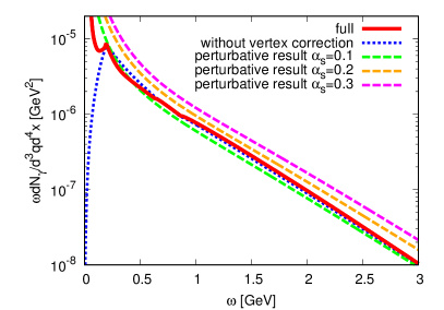
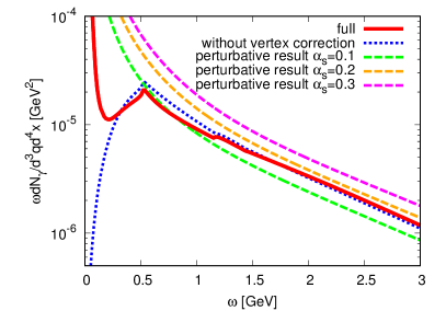
Next, let us see the numerical results on the photon production spectrum. In Fig. 6, we show the photon production rate with the lattice quark propagator and the gauge invariant vertex as a function of the photon energy $\omega$ for $T=1.5T_{\rm c}$ by the solid line. The production rate with the bare vertex obtained in Sec. III.1 is also plotted by the dotted line. The photon production rate has been calculated in the perturbative analysis Arnold:2001ba ; Arnold:2001ms ; Ghiglieri:2013gia . In the figure, we show fitting formula for the perturbative result in Refs. Arnold:2001ba ; Arnold:2001ms for three values of the strong coupling constant $\alpha_{s}=0.1,0.2$, and $0.3$ by the dashed lines; this fitting function well reproduces the complete leading log result for $0.2\leq\omega/T\leq 50$ Arnold:2001ms . The next-to-leading order result Ghiglieri:2013gia enhances the rate at most 20% around $\omega/T\sim 2$.

From Fig. 6, one finds that the production rates with full and bare vertices behave similarly for $\omega\gtrsim 0.2$ GeV. This result suggests that the effect of the vertex correction is not large. The figure also shows that the production rate with the lattice quark propagator behaves quite similarly with the perturbative result with $\alpha_{\rm s}\simeq 0.1-0.2$ except for low energy region. This result is unexpected, because the production mechanisms of photons are different between these analyses.

Figure 6: Photon production rate for $T=1.5T_{\rm c}$. The result without vertex correction is expressed by the dotted line and perturbative results are plotted with the dashed lines.

As discussed in the previous section, the photon production rate can be decomposed into contributions of different processes. In Fig. 7, we show the contributions of each term in Eq. (42) on the production rate. In the figure, the lines show the rate from the pair annihilation of a normal and a plasmino modes (PA($\nu_{+}\nu_{-}$)) and two plasmino modes (PA($\nu_{-}\nu_{-}$)), the Landau damping between a normal and a plasmino modes (LD($\nu_{+}\nu_{-}$)) and two plasmino modes (LD($\nu_{-}\nu_{-}$)), the rates of two anomalous productions (Anom.($V\nu_{+}$) and Anom.($V\nu_{-}$)), and the total (full) rate. The figure shows that the photon production for $\omega\lesssim 1.5$ GeV is dominated by the Landau damping LD($\nu_{+}\nu_{-}$), while for higher energies two production mechanisms LD($\nu_{+}\nu_{-}$) and PA($\nu_{+}\nu_{-}$) have almost the same contributions. The process LD($\nu_{-}\nu_{-}$) is interpreted as the Cherenkov radiation from the acausal dispersion relation of the plasmino mode. From Fig. 7, one finds that the photon production with this process is well suppressed except for $\omega\lesssim 0.2$ GeV. This result shows that the effect of this unphysical process is negligible. The figure also shows that the contribution of the anomalous productions (Anom.($V\nu_{+}$) and Anom.($V\nu_{-}$)) are small compared to other processes except for the low energy region $\omega\lesssim 0.2$ GeV. The decomposition of the photon production rate obtained with the bare vertex, Eq. (28), shows the similar tendency as the one of the full result.

Figure 7: Decomposition of the photon production rate for $T=1.5T_{\rm c}$.

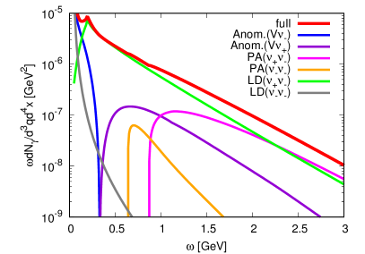
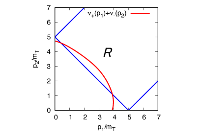
Figure 7 shows that the processes PA$(\nu_{+}\nu_{-})$ and PA$(\nu_{-}\nu_{-})$ take nonzero values for $\omega>\omega_{+-}$ and $\omega_{--}$, respectively, with $\omega_{+-}\simeq 0.86$ GeV and $\omega_{--}\simeq 0.63$ GeV. Owing to the emergence of these processes, the total production rate has non-smooth behaviors at these energies. To understand the reason why these processes emerge at $\omega=\omega_{+-}$ and $\omega_{--}$, in Fig. 8 we show the minimum of the photon energy produced by these processes with a fixed photon momentum $q$. In the figure, the minimum energy for the pair annihilation of two normal modes ($\nu_{+}\nu_{+}$) is also plotted for comparison. In the regions above the lines, virtual photon production is allowed kinematically. From the figure, one finds that the region covers even a part of the space-like region for $\nu_{+}\nu_{-}$ and $\nu_{-}\nu_{-}$, and thus these processes can produce a real photon, while the region for $\nu_{+}\nu_{+}$ does not have an overlap with the light cone. The real photon production from two quasi-particle pair annihilation does not occur in the perturbative calculation based on the hard thermal loop resummation technique, because the normal and plasmino modes in this formalism exists only in the time-like region. The lattice propagator, on the other hand, has the plasmino mode which enters space-like region as in Fig. 2. This behavior is responsible for the emergence of the nonzero production rates by PA$(\nu_{+}\nu_{-})$ and PA$(\nu_{-}\nu_{-})$.

Figure 8: Dispersions of photons produced via quasi-particle pair annihilations. Each line shows the minimum value of dispersions. Dotted line is the light cone.

The photon spectra shown in Fig. 6 has a cusp structure at $\omega=\omega_{\rm max}$ with $\omega_{\rm max}\simeq 0.2$ GeV. According to Fig. 7, this cusp comes from the Landau damping LD($\nu_{+}\nu_{-}$). The origin of this structure is understood from the kinematics between quasi-particle pair and photon. Let us denote the momenta of the normal and plasmino modes $\bm{p}_{+}$ and $\bm{p}_{-}$, respectively, and the photon momentum $\bm{q}$. Then, these momenta satisfy $\bm{p}_{+}=\bm{p}_{-}+\bm{q}$. For $\omega<\omega_{\rm max}$, the decay process is allowed for all directions of quark momenta. At $\omega=\omega_{\rm max}$, the process with perpendicular $\bm{p}_{+}$ and $\bm{q}$, i.e. the case with $|\bm{p}_{+}|+|\bm{q}|=|\bm{p}_{-}|$ starts to be forbidden kinematically, and the phase space becomes narrower as $\omega=|\bm{q}|$ becomes larger. This constraint in the phase space gives rise to the cusp in the production spectrum.

It is a surprising result that the photon production spectrum in our analysis has a similar behavior, not only in the slope but also the absolute value, as the perturbative results for almost all energy range. The slopes in both results are approximately given by the Boltzmann factor ${\rm e}^{-\beta\omega}$. The origin of this slope in our analysis can be understood as follows. From Fig. 7, the photon production is dominated by two processes, PA($\nu_{+}\nu_{-}$) and LD($\nu_{+}\nu_{-}$). These processes include the plasmino mode whose residue $Z_{-}$ is exponentially damping for large momentum. Because of this factor, the momentum of the plasmino mode must be small, $\bm{p}_{-}\simeq 0$. Then, to produce a real photon with large momentum $|\bm{q}|\gg m_{\rm T}$, the momentum of the normal mode must satisfy $\bm{p}_{+}=\bm{q}\pm\bm{p}_{-}\simeq\bm{q}$, and the photon emission takes place via the decay of this mode. The rate of this process is proportional to the thermal probability of the existence of the normal mode given by ${\rm e}^{-\beta\nu_{+}(q)}\simeq{\rm e}^{-\beta q}={\rm e}^{-\beta\omega}$. For sufficiently large $\bm{q}$, this factor determines the production rate, because other effects, such as the phase space determined by kinematics and $Z_{+}(|\bm{p}_{+}|)\simeq 1$, are insensitive to $\bm{q}$. In the perturbative analysis, the photon self-energy at high energy is dominated by two-loop diagrams and collinear enhanced diagrams Arnold:2001ms . In these processes, an initial quark with large momentum $\bm{q}$ must decay into soft degrees of freedom, and the Boltzmann factor appears for the same reason as ours, while it is known that other factors are insensitive to $\bm{q}$ Arnold:2001ms . To summarize, the coincidence in the slope comes from the thermal factor for the initial quark with large momentum. Because the decay processes in these analyses are completely different, however, the coincidence in magnitude would be accidental.

In Fig. 9, we show the result for $T=3T_{\rm c}$. Its behavior is qualitatively the same as the production rate for $T=1.5T_{\rm c}$, although the spectrum has a clearer dip structure at low energy $\omega\simeq 0.5$ GeV. The contributions of different decay processes behave similarly, too.

The results at both temperatures have a similar form and magnitude with the perturbative results. If a closer look is taken, however, we recognize that our non-perturbative results are almost reproduced by perturbative results with $\alpha_{\rm s}\simeq 0.1-0.2$, which is rather on the lower side. This has an important phenomenological consequence; the discrepancy between the observed photon yield at RHIC and the corresponding theoretical result is not resolved, but is enlarged. Thus, it is confirmed also by this investigation that there will exist still unknown mechanisms for photon production in relativistic heavy ion collisions.

Figure 9: Photon production rate for $T=3T_{\rm c}$. The result without vertex correction is expressed by the dotted line. Perturbative results are plotted with the dashed lines for three values of $\alpha_{s}$.

V Summary

In this paper, we analyzed the production spectrum of thermal photons from the deconfined medium near the critical temperature $T_{\rm c}$. In order to include the non-perturbative effect in the analysis, we analyzed the Schwinger-Dyson equation of the photon self-energy with the quark propagator obtained on the lattice for two temperatures. The photon-quark vertex is constructed so as to satisfy the WTI. The effect of the vertex correction is discussed. We showed that the vertex function satisfying the WTI generates anomalous photon production mechanisms but its contribution is small. In comparison with the perturbative analysis, the spectra with the lattice quark propagator show almost the same behavior for $\omega\gtrsim 0.5$ GeV. We discussed that the coincidence in the slope can be understood from the production mechanism. However, it is a nontrivial result that the our result is similar to the perturbative one even in the magnitude. The gap between experimental data and theoretical calculations on the yield and flows of photons still remain. Our result indicates the existence of unknown mechanisms of photon production in relativistic heavy ion collisions.

The authors thank T. Shimoda, K. Ogata, and K. Oda for encouragements. T. K. is supported by Grant-in-Aid for JSPS research fellows (No. 16J00981) and Osaka University Cross-Boundary Innovation Program. This work is supported in part by JSPS KAKENHI Grant Numbers 26400272 and 17K05442.

References

- (1) I. Arsene et al. [BRAHMS Collaboration], Nucl. Phys. A 757, 1 (2005); B. B. Back, et al. [PHOBOS Collaboration], ibid. 757, 28 (2005); J. Adams et al. [STAR Collaboration], ibid. 757, 102 (2005); K. Adcox et al. [PHENIX Collaboration], ibid. 757, 184 (2005).
- (2) B. Muller, J. Schukraft, and B. Wyslouch, Ann. Rev. Nucl. Part. Sci. 62, 361 (2012).
- (3) A. Adare et al. [PHENIX Collaboration], Phys. Rev. C 91, no. 6, 064904 (2015).
- (4) J. Adam et al. [ALICE Collaboration], Phys. Lett. B 754, 235 (2016).
- (5) A. Adare et al. [PHENIX Collaboration], Phys. Rev. C 94, no. 6, 064901 (2016).
- (6) J. F. Paquet, C. Shen, G. S. Denicol, M. Luzum, B. Schenke, S. Jeon and C. Gale, Phys. Rev. C 93, no. 4, 044906 (2016).
- (7) C. Shen, U. W. Heinz, J. F. Paquet, I. Kozlov and C. Gale, Phys. Rev. C 91, no. 2, 024908 (2015).
- (8) J. I. Kapusta, P. Lichard and D. Seibert, Phys. Rev. D 44, 2774 (1991); Erratum-ibid. 47, 4171 (1993).
- (9) R. Baier, H. Nakkagawa, A. Niegawa and K. Redlich, Z. Phys. C 53, 433 (1992).
- (10) P. B. Arnold, G. D. Moore and L. G. Yaffe, JHEP 0111, 057 (2001).
- (11) P. B. Arnold, G. D. Moore and L. G. Yaffe, JHEP 0112, 009 (2001).
- (12) J. Ghiglieri, J. Hong, A. Kurkela, E. Lu, G. D. Moore and D. Teaney, JHEP 1305, 010 (2013).
- (13) T. Hirano and M. Gyulassy, Nucl. Phys. A 769, 71 (2006).
- (14) T. Hirano, U. W. Heinz, D. Kharzeev, R. Lacey and Y. Nara, Phys. Lett. B 636, 299 (2006).
- (15) L. D. McLerran and T. Toimela, Phys. Rev. D 31, 545 (1985).
- (16) H. A. Weldon, Phys. Rev. D 42, 2384 (1990).
- (17) C. Gale and J. I. Kapusta, Nucl. Phys. B 357, 65 (1991).
- (18) F. Karsch and M. Kitazawa, Phys. Lett. B 658, 45 (2007).
- (19) F. Karsch and M. Kitazawa, Phys. Rev. D 80, 056001 (2009).
- (20) O. Kaczmarek, F. Karsch, M. Kitazawa and W. Soldner, Phys. Rev. D 86, 036006 (2012).
- (21) T. Kim, M. Asakawa and M. Kitazawa, Phys. Rev. D 92, no. 11, 114014 (2015).
- (22) A. K. Rebhan, Phys. Rev. D 48, R3967 (1993).
- (23) L. D. Landau, J. Phys. (USSR) 10, 25 (1946).
- (24) J. S. Ball and T. W. Chiu, Phys. Rev. D 22, 2542 (1980).
- (25) M. Le Bellac, Thermal Field Theory (Cambridge University Press, Cambridge, 1996).