Nonlinear structures and anomalous transport in partially magnetized $\mathbf{\ E\times B}$ plasmas.

Abstract

Nonlinear dynamics of the electron-cyclotron instability driven by the electron $\mathbf{\ E\times B}$ current in crossed electric and magnetic field is studied. In nonlinear regime the instability proceeds by developing a large amplitude coherent wave driven by the energy input from the fundamental cyclotron resonance. Further evolution shows the formation of the long wavelength envelope akin to the modulational instability. Simultaneously, the ion density shows the development of high-k content responsible for wave focusing and sharp peaks on the periodic cnoidal wave structure. It is shown that the anomalous electron transport (along the direction of the applied electric field) is dominated by the long wavelength part of the turbulent spectrum.

I Introduction

Partially magnetized weakly collisional plasmas with magnetized electrons and weakly magnetized ions are abundant in nature and laboratory conditions. Therefore, their nonlinear behavior is of considerable interest for fundamental physics and applications. One of the most common examples is a plasma discharge driven by transverse current perpendicular to the magnetic field, Buneman (1962); Arefev, Gordeev, and Rudakov (1969); Wong (1970); Gary and Sanderson (1970) either due to free streaming of unmagnetized ions across the magnetic field or due to the electron drift current in crossed electric and magnetic field, $\mathbf{V}_{E}=\mathbf{\ E\times B/}B^{2}$. Such configurations are relevant to collisionless shock waves in space, pulsed power laboratory devices, Penning discharges and various devices for material processing and space propulsion. Plasmas with crossed $\mathbf{E}\times\mathbf{B}$ fields are subject to a variety of instabilities such as ion-sound, lower-hybrid and Simon-Hoh modes which may be driven by plasma density, magnetic field and temperature gradients as well as collisions Lashmore-Davies and Martin (1973); Smolyakov et al. (2017); Davidson and Krall (1977). The electron cyclotron drift instability is of particular interest because it does not require any gradients and may be active in a homogeneous collisionless plasma with electric field perpendicular to the magnetic field.Sizonenko and Stepanov (1967); Gary and Sanderson (1970); Wong (1970) Large-amplitude waves present in satellite observations of bow shock crossings have been associated with current driven electron-cyclotron instabilities.Wilson et al. (2010, 2014a, 2014b); Breneman et al. (2013) Presence of the electron cyclotron instabilities has been confirmed by numerical simulations of bow shocks. Muschietti and Lembège (2006, 2013); Matsukiyo and Scholer (2006)

There have been a number of earlier studies Biskamp and Chodura (1971, 1972, 1973); Forslund, Morse, and Nielson (1970); Lampe et al. (1971, 1971); Lominadze (1972) addressing linear and nonlinear theory of the electron-cyclotron instabilities, but many critical questions remained unresolved. Recent developments in applications of $\mathbf{E\times B}$ discharges (also referred as $\mathbf{E\times B}$ plasma below) such as HiPIMPS magnetrons, Hall thrusters and Penning discharges have again raised questions on the nature of turbulence, transport and nonlinear structures in such conditions Tsikata and Minea (2015); Smirnov, Raitses, and Fisch (2006); Adam, Heron, and Laval (2004); Boeuf and Chaudhury (2013); Boeuf (2014, 2017).

Linearly, the electron-cyclotron instability is based on the interaction of the electron cyclotron mode with ion plasma oscillations. Both dissipative and reactive regimes may occur. In the dissipative regime, the negative energy wave is excited due to resonance absorption of wave energy by electron and ions.Sizonenko and Stepanov (1967) The reactive instability may occur due to coupling of waves with positive and negative energy.Lashmore-Davies (1970); Biskamp and Chodura (1972) For propagation strictly perpendicular to the magnetic field and electrons subject to $\mathbf{E\times B}$ drift, the resonant condition is $\omega-\mathbf{k\cdot v}_{E}-m\Omega_{ce}=0$. It has been noted that electron cyclotron drift instability (ECDI) due to linear and/or nonlinear effects Sizonenko and Stepanov (1967); Arefev (1970); Lashmore-Davies and Martin (1973); Lampe et al. (1971, 1972a) may in some regimes become similar to the ion-sound instability in unmagnetized plasmas. The transition of the ECDI instability, which in essential way depends on the presence of the magnetic field, into the regime which resembles the ion sound instability in absence of the magnetic field has become a common theme of many earlier works in the literature Lampe et al. (1972b, a). In recent years, the regime of unmagnetized ion sound turbulence has been considered as a main paradigm for nonlinear regime of the electron cyclotron drift instability — in particular — for calculations of the associated anomalous current in Hall thrusters Katz et al. (2015); Cavalier et al. (2013); Lafleur, Baalrud, and Chabert (2016a, b).

The goal of this paper is to investigate the nonlinear regime of the ECDI instability, its possible transition to the unmagnetized ion-sound regime, and associated level of the anomalous transport. We show here that for typical plasma parameters relevant to applications to magnetron and Hall thruster plasmas, the ion-sound like regime of the ECDI (with fully demagnetized electrons) does not occur, even in absence of energy losses for electrons. The magnetic field continues to play an important role in the electron dynamics, particularly in the energy supply to the mode and electron heating mechanism. Nonlinearly the instability continues to exist as coherent mode at the fundamental cyclotron resonance $k_{0}\equiv v_{E}/\Omega_{ce}$. Interestingly, electron demagnetization during ECDI has recently been discussed in applications to the collisionless bow shock plasma of the Earth.Muschietti and Lembège (2013) Nonlinear simulations of Ref. Muschietti and Lembège, 2013 have also shown that the fundamental cyclotron resonance remains active and no full demagnetization occurs.

Our results also demonstrate that the injected energy (primarily at the lowest resonance) cascades toward even longer wavelength modes. This inverse energy cascade (toward longer wavelengths) is characterized by the formation of a long wavelength envelope, similar to the modulational instability of the wave packets. We posit that the slow long wavelength envelope discovered in our simulations is responsible for low frequency structures exhibited by ECDI instability recently observed experimentally in high-power pulsed magnetron (HIPIMS) discharge.Tsikata and Minea (2015) We investigate the anomalous current and find that it is dominated by the long-wavelength modes.

II Linear dispersion relation

In this section we discuss main features of the electron-cyclotron drift instability (ECDI) with respect to the linear dispersion relation that was obtained in a number of earlier works.Gary and Sanderson (1970); Wong (1970); Arefev (1970) We consider a plasma immersed in the crossed electric and magnetic field, $\mathbf{E}=E_{0}\widehat{\mathbf{z}}$, $\mathbf{B}_{0}=B_{0}\widehat{\mathbf{y}}$. The ions are unmagnetized, but electrons are magnetized and experience the $\mathbf{E\times B}$ drift, $\mathbf{v}_{E}=-E_{0}/B_{0}\widehat{\mathbf{x}}$. One-dimensional fluctuations are propagating in the $x$ direction, $\mathbf{k}=k\widehat{\mathbf{x}}$. The linear kinetic dispersion relation Gary and Sanderson (1970); Wong (1970); Arefev (1970) has the form $1+K_{i}+K_{e}=0$, where the ion response is $K_{i}=-1/\left(2k^{2}\lambda_{Di}^{2}\right)Z^{{}^{\prime}}\left(\omega/\sqrt{2}kv_{i}\right)$, and the electrons are described by

$$K_{e}=\frac{1}{k^{2}\lambda_{De}^{2}}\left[1-\exp\left(-k^{2}\rho_{e}^{2}\right)I_{0}\left(k_{\bot}^{2}\rho_{e}^{2}\right)\right.$$

$$\left.-2\left(\omega-k_{x}v_{E}\right)^{2}\sum\limits_{m=1}^{\infty}\frac{\exp\left(-k_{\bot}^{2}\rho_{e}^{2}\right)I_{m}\left(k_{\bot}^{2}\rho_{e}^{2}\right)}{\left(\omega-k_{x}v_{E}\right)^{2}-m^{2}\Omega_{ce}^{2}}\right]$$ (1)

where $\Omega_{ce}=eB/m_{e}$, $\lambda_{D\alpha}=\varepsilon_{0}T_{\alpha}/\left(e^{2}n_{0}\right)$, $v_{\alpha}=\sqrt{T_{a}/m_{a}}$ for species $\alpha$, $I_{m}$ is the modified Bessel function of the first kind, and $Z(z)$ is the plasma dispersion function.

Unstable eigenmodes form a discrete set of modes localized near the resonances $\omega-kv_{E}=m\Omega_{ce}$. In the cold plasma limit, only the lowest $m=1$ resonance exists and Eq. (II) reduces to the reactive Buneman instability Buneman (1962) with the dispersion relation $1=\omega_{pi}^{2}/\omega^{2}+\omega_{pe}^{2}/\left(\left(\omega-kv_{E}\right)^{2}-\Omega_{ce}^{2}\right)$, which was discussed as a mechanism of anomalous transport in $\mathbf{E\times B}$ discharges in Refs. Baranov et al., 1996; Adam, Heron, and Laval, 2004. The finite electron temperature makes $m=1$ resonance narrow and opens up higher $m$ resonances at $kv_{E}\simeq m\Omega_{ce}$. The growth rates of the higher resonance modes are first increasing with $m$ and then decrease for high $m$. The width of the resonances decreases with temperature Lominadze (1972); Lashmore-Davies (1970). A detailed structure and behavior of the linear eigenmodes from Eq. (II) was investigated in a number of papers, such as in Refs. Gary and Sanderson, 1970; Lominadze, 1972; Adam, Heron, and Laval, 2004; Ducrocq et al., 2006; Cavalier et al., 2013. A recent discussion of properties of the linear ECDI instability can also be found in Ref. Muschietti and Lembège, 2013.

III Nonlinear dynamics and formation of the long-wavelength envelope

Nonlinear dynamics of the ECDI instability is studied here with 1D3V parallel particle-in-cell simulations using the PIC code EDIPIC Sydorenko (2006). As a characteristic example we consider a xenon plasma ($m_{Xe}=131.293\,\text{amu}$) with Hall-effect thruster relevant parameters of $n_{0}=10^{17}\,\text{m}^{-3}$, $E_{0}=20\,\text{kV/m}$, $B_{0}=0.02\,\text{T}$, initial temperatures of $T_{e}=10\,\text{eV}$ and $T_{i}=0.2\,\text{eV}$, simulation box length $L=44.56\,\text{mm}$ using a spatial resolution in $x$ of $\lambda_{De}/8$, and the initial electron Larmor radius of $0.5\,\text{mm}$. The wave vector is constrained by periodicity of the simulation domain to $k\,L=2\pi\,n$, where $L=2\pi r$ is the azimuthal length of the channel (or periodic portion thereof). The particles are initialized as Maxwell-Boltzmann distributions, shifted by the $\mathbf{E}\times\mathbf{B}$ drift velocity $v_{E}$ for the electrons. Time step is chosen to fulfill the CFL condition for particles up to $35v_{e}$ from the initial value, and $10^{4}$ marker particles per cell are used for a noise level of 1% or less.

The linear instability commences with the growth of the most unstable linear cyclotron harmonic (for our parameters here $m=3$ and $n=6$). At a later time, the progressively lower $k$ cyclotron harmonics take over as Figs. 1 and 2 illustrate.

In part, the downward shift occurs due to increase of the electron temperature as a result of the heating Muschietti and Lembège (2013). In nonlinear stage however this tendency is amplified by the inverse cascade which shifts energy further down to large scales much below of the length scale of the fundamental cyclotron mode $k_{0}^{-1},k_{0}=\Omega_{ce}/v_{E}$, as evidenced in Fig. 2 as well as by the modulation of the wave envelope in Figs 3 and 4. Note that in our simulations modes corresponding to the few lowest cyclotron harmonics with $m<10$ remain to be clearly present well into the nonlinear stage as seen in Fig. 2.

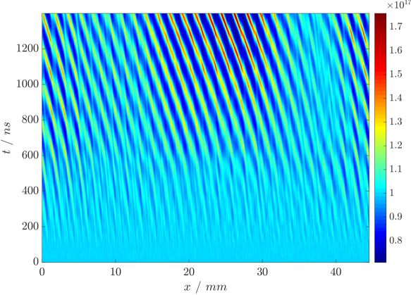
Figure 1: Ion density as a function of time. Note the simultaneous appearance of the cnoidal structure along with modulation.

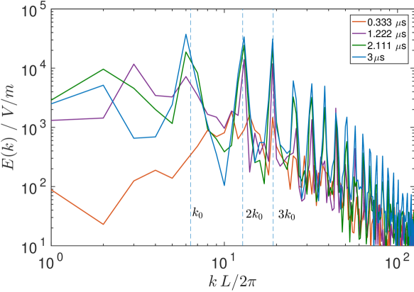
Figure 2: Amplitudes of $E_{x}$ spectral components over the simulation time. First three cyclotron harmonics are shown as vertical lines. Significant sub-resonant components are seen below the lowest cyclotron harmonic, and an upward cascade to lower $k$.

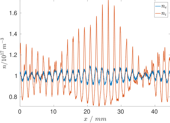
Figure 3: Ion and electron density shown at $1.4\,{\mu}\text{s}$. Note the cnoidal structure of ion density fluctuations.

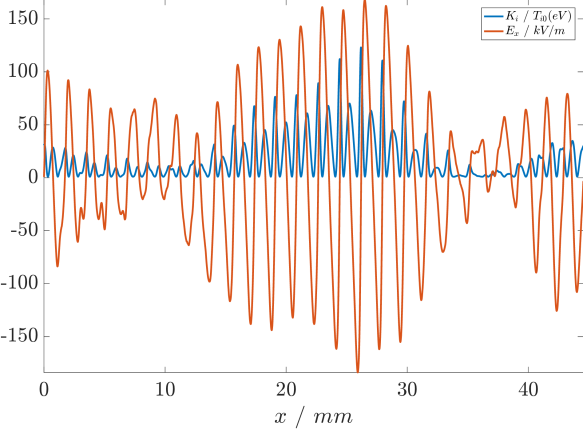
Figure 4: Electric field and ion temperature at $1.4\,{\mu}\text{s}$.

The $\mathbf{E\times B}$ instability described above is a very effective mechanism for electron heating due local trapping and detrapping in the time dependent potential formed by the magnetic field and the wave field .Biskamp and Chodura (1972); Forslund et al. (1972); Forslund, Morse, and Nielson (1970) Even when initiated with almost cold electrons of $T_{e}=0.001\,\text{eV}$, the electron temperature rises to $T_{e}=20$ eV within few $\gamma^{-1}\simeq\omega_{LH}^{-1}$. Within this time range, the instability changes from the linear exponential growth to the slower growth in which the potential energy and electron temperature increase at the same rate approximately linearly in time, as shown in Fig. 5. The electron heating is manifested as intense phase-space mixing of the electron distribution function which becomes flattened.Ducrocq et al. (2006) The flattening of the distribution can be visualized through the excess kurtosis of the distribution function, defined as $\text{Kurt}(f)=\int{(x-\mu)^{4}f(x)/\sigma^{4}}\,dx-3$, with mean $\mu$ and variance $\sigma^{2}$. It becomes apparent from Fig. 6 that heating has flattened the distribution away from the Maxwell-Boltzmann statistics, and caused a slight asymmetry in the $x-z$ temperatures. The development of finite excess kurtosis and change of the distribution from Maxwellian (with kurtosis 3) to platykurtic (kurtosis of less than 3), which occur at $t\approx 100\,\text{ns}$, Fig. 4, mark the transition from the linear exponential growth to the slower nonlinear regime. The flattened distribution is also observed in the ionosphere, like in Ref. Mozer and Sundkvist, 2013.

In the nonlinear regime the perturbed electric field develops into a robust quasi-coherent mode with a primary wave vector around the fundamental cyclotron resonance.Boeuf (2014) The growing mode is driven by the energy input from the few lowest order cyclotron resonances with $k_{0}$ providing the dominant contribution, as seen in Fig. 4. The electron density, Fig. 3, is modulated mostly at $k=k_{0}$. The ion dynamics has more complex structure showing nonlinearly generated high-$k$ modes and ion trapping (bunching) features typical for large amplitude nonlinear waves.Davidson (2012) Features of the localized ion trapping are further seen in the comparison of the electric field and ion energy profiles, Fig. 2, as well as in the electric field structures correlated with the ion energy fluctuations, Fig. 2. A characteristic nonlinear cnoidal wave structure of the ion density, Fig. 3, is further confirmed by the equal spacing of peaks in the $k$ and $\omega$ spectra in figures 2 and 8, respectively.

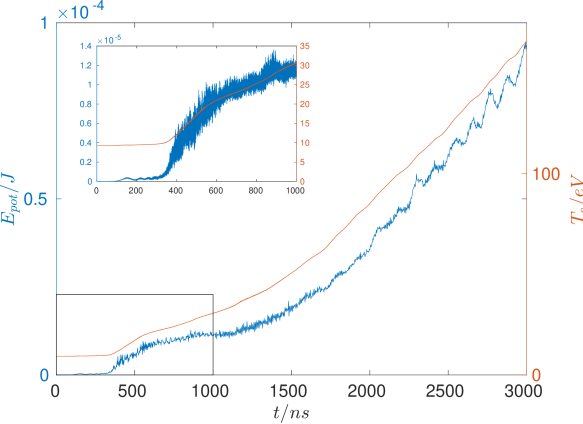
Figure 5: Potential energy and electron temperature in the simulation.

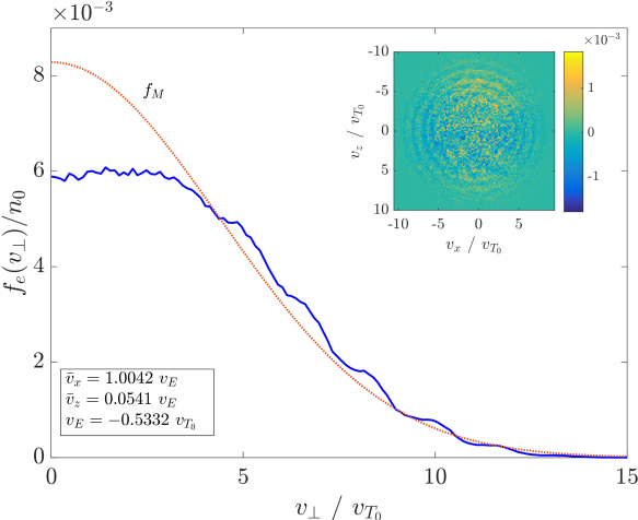
Figure 6: Distribution function of electrons at $t=1.4\mu{s}$, with annular patterns apparent due to heating. The gyro-angle dependent part is shown in the insert. Here $v_{x}$ is the velocity in $E\times B$ direction (in units of the $v_{E}$), $v_{z}$ is in the direction of the background electric field, and $v_{\text{th}}$ is electron thermal velocity. The Maxwellian distribution ($f_{M}$) given as reference has the same temperature and volume as the measured one.

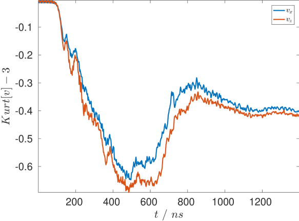
Figure 7: Excess kurtosis ($4^{\text{th}}$ central moment) for the electron distribution over time. Note the slight asymmetry for $v_{x}$ and $v_{z}$.

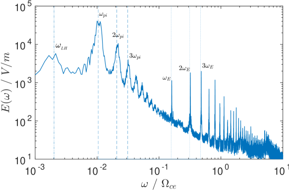
Figure 8: Maximal amplitudes for the $\omega$-spectrum for $E_{x}$, $\omega_{E}=V_{e}2\pi/L$.

The fluctuation spectra remain well quantized and predominantly retain the fundamental cyclotron mode structure. However, one can also see the development of a long wavelength envelope in the density fluctuations analogous to the typical picture of the modulational instability which is another evidence of the inverse cascade. The modulations and cnoidal features increase in time, as shown in figures 1 and 4.

IV Demagnetization of the electron motion and transition to the ion sound modes

Many studies of the ECDI instability have emphasized the effects of demagnetization of electrons and the transition of the mode into the regime of the ion-sound instability that occurs in the absence of a magnetic field. It is important to note that the mode structure and demagnetization mechanism is a sensitive function Arefev (1970); Lashmore-Davies and Martin (1973); Lampe et al. (1971) of the $k_{y}v_{e}$ parameter, where $k_{y}$ is the wave vector along the magnetic field. Here we consider the case of strictly perpendicular propagation, $k_{y}=0$.

The demagnetization of electron dynamics for large values $k^{2}\rho_{e}^{2}$ can be easily seen from equation (II). In the limit $k^{2}\rho_{e}^{2}\gg 1$, the contribution of the terms $\exp\left(-k^{2}\rho_{e}^{2}\right)I_{m}\left(k^{2}\rho_{e}^{2}\right)\rightarrow 1/\left(k\rho_{e}\right)$ for all $m=0,1,...$ is neglected and the electron response in Eq. (II) becomes $K_{e}=\left(k^{2}\lambda_{De}^{2}\right)^{-1}$, which corresponds to the Boltzmann response of unmagnetized electrons.

The electron demagnetization in the linear short wavelength regime $k\rho_{e}\gg 1$ can be viewed as the transition of the lower-hybrid mode (propagating strictly perpendicular to the magnetic field) to the “high-frequency ion-sound”. Indeed, the dispersion relation for the quasi-neutral lower hybrid mode with warm electrons has the form Smolyakov et al. (2017) $\omega^{2}=\omega_{LH}^{2}\left(1+k_{\bot}^{2}\rho_{e}^{2}\right)$. It is easy to see that in the short wavelength regime with $k_{\bot}^{2}\rho_{e}^{2}\geq 1$, the mode dispersion relation becomes $\omega^{2}=\omega_{LH}^{2}k_{\bot}^{2}\rho_{e}^{2}=k_{\bot}^{2}c_{s}^{2}$. The lower hybrid mode is present in the measured frequency spectrum, as shown in Fig. 8.

The neglect of all $m=1,2,3..$ cyclotron harmonics in Eq. (II) may be justified for large $k\rho_{e}\gg 1$, but not near the cyclotron resonances, $\left[\left(\omega-k_{x}v_{E}\right)^{2}-m^{2}\Omega_{ce}^{2}\right]\rightarrow 0$, where these terms cannot be neglected. Therefore the mode properties may be close to the lower-hybrid/ion sound mode which is determined by the first two terms in Eq. (II), but the mode drive is determined by the resonance $\left[\left(\omega-k_{x}v_{E}\right)^{2}-m^{2}\Omega_{ce}^{2}\right]\rightarrow 0$, where the $m=1$ is the most important. This resonance condition fixes the wavelength of the coherent mode at $k_{0}=\Omega_{ce}/v_{E}$. Note that in simulations the measured phase velocity of the coherent wave turns out to be of the order of the ion sound velocity within a factor of 2.

Deviations from quasi-neutrality bring in the effects of the electron Debye length (or, Debye shielding), similar to the ion sound modes in the short wavelength regime $\omega^{2}=k^{2}c_{s}^{2}/(1+k^{2}\lambda_{D}^{2})$ so that $\omega\rightarrow\omega_{pi}$ for $k^{2}\lambda_{D}^{2}>1$. The short wavelength structures in the ion density are seen in the sharp peaks of ion density which contain high $k$ modes (Figs. 3 and 1) and explain the $\omega_{pi}$ (and its harmonics) peaks in the amplitude spectrum, as shown in Fig. 8.

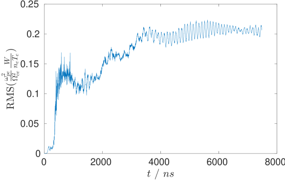
Figure 9: Parameter $\Xi$ in the condition for turbulent destruction of cyclotron resonances: $\Xi>\left(k\rho_{e}\right)^{-1}$.

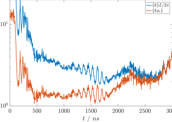
Figure 10: Energy weighted averages of $k$ and $k\rho_{e}$ from anomalous current over time. See text for definition.

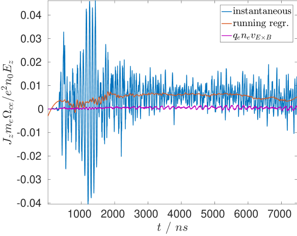
Figure 11: Mean anomalous current density over time, instantaneous value and a 2nd order running regression using a window much larger than the oscillation frequency, shown with the concurrent $E\times B$ flux. The latter is negligible.

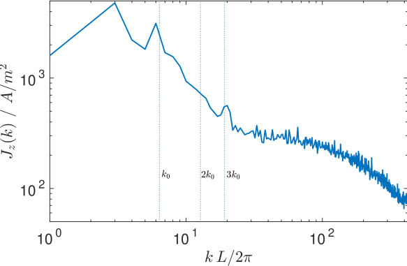
Figure 12: Maximal amplitudes of the anomalous current $J_{z}$ as a function of the wave vector $k$ over the simulation. The sub-resonant (lower than $k_{0}=\Omega_{ce}/v_{E}$) components are observed to dominate over linearly resonant values. Note the finite value at system size.

The cyclotron resonances can be destroyed by collisions even for $\nu/\Omega_{ce}<1$ Pitaevskii (1963); Huba and Ossakow (1979). The collisions destroy the resonances when the particle diffuses by the distance $\lambda/2=\pi/k$ over the period of the cyclotron rotation $\tau_{c}=2\pi/\omega_{c}$, or when $\delta R=\left(D_{c}\tau_{c}\right)^{1/2}>\lambda/2$. For the collisional diffusion with $\nu<\omega_{c}$, $D_{c}=\nu\rho_{e}^{2}$, thus the collisions will destroy cyclotron resonances for $\left(\nu/\Omega_{ce}\right)k^{2}\rho_{e}^{2}>\pi/2$.

A number of previous works have argued that nonlinear effects can also effectively demagnetize the electrons via the anomalous resonance broadening Dum and Sudan (1969). A simple criterion for this may be obtained as follows. Let us consider short wavelength modes with $k\rho_{e}\gg 1$. In this regime, the electron experiences $N=2\pi\rho_{e}/\lambda$ scattering events or “collisions” during one period of the cyclotron rotation. Each “collision” represents a small angle scattering with velocity change $\delta v$: $m_{e}v_{e}\delta{v}=e\delta{\phi}$. During such a ”collision” the electron guiding center is shifted by the distance: $\delta r=\delta v/\Omega_{ce}$. Each “collision” is random and the net displacement $R$ over the time $\tau_{c}=2\pi/\Omega_{ce}$ is $R=\delta rN^{1/2}$, giving the effective nonlinear diffusion coefficient $D_{nl}=R^{2}/\tau_{c}=\Xi v_{Te}\lambda/4$, where $\Xi\equiv\left(\omega_{pe}^{2}/\Omega_{ce}^{2}\right)W/\left(n_{0}T_{e}\right)$, $W=E^{2}/8\pi$, where we have used $\delta\phi=E\lambda/2$, $v_{e}=v_{Te}\equiv\left(2T_{e}/m_{e}\right)^{1/2}$. The cyclotron resonances will be destroyed when over one cyclotron period $\tau_{c}$ the particle is displaced due to nonlinear diffusion by a distance larger than the half-wavelength, $\left(D_{nl}\tau_{c}\right)^{1/2}>\lambda/2$. This gives the criterion of nonlinear destruction of cyclotron resonances as $\Xi>\left(k\rho_{e}\right)^{-1}$.Biskamp and Chodura (1973); Lampe et al. (1972a)

Alternatively, the effects of nonlinear resonance broadening can be described by the addition of the nonlinear diffusion term $ik^{2}D_{nl}$ into $K_{e}$ in Eq. (II). For large $k^{2}\rho_{e}^{2}$, $\exp\left(-k^{2}\rho_{e}^{2}\right)I_{m}\left(k^{2}\rho_{e}^{2}\right)=1/\left(k\rho_{e}\right)$, the summation of all cyclotron harmonics can be performed giving Lampe et al. (1971)

$$K_{e}^{nl} = \frac{1}{k^{2}\lambda_{De}^{2}}\left[1+\left(\frac{\pi}{2}\right)^{1/2}\frac{\left(\omega-kv_{E}\right)}{kv_{e}}\right.\times$$ (2)

$$\times\cot\left.\left(\pi\frac{\omega-kv_{E}+ik^{2}D_{nl}}{\Omega_{ce}}\right)\right].$$

For $k^{2}D_{nl}>\Omega_{ce}$, which is equivalent to the condition $\left(D_{nl}\tau_{c}\right)^{1/2}>\lambda/2)$, $\cot\left(ik^{2}D_{nl}/\Omega_{ce}\right)\simeq-i$ and the equation (2) corresponds to the response of unmagnetized electrons.

The destruction of cyclotron resonances was considered in Ref. Lampe et al., 1971 as the main nonlinear effect resulting in saturation of electron cyclotron instability and transition to the regime of slower ion sound instability in absence of the magnetic field. In the course of the nonlinear evolution of the instability the wave and electron thermal energy grow simultaneously, Fig. 5. As a result, the parameter $\Xi$ remains well under unity so that the condition $\Xi>\left(k\rho_{e}\right)^{-1}$ is typically not satisfied, Fig. 9. Note that the effective $k\rho_{e}$ in our simulations remains of the order of unity, Fig. 10. The persistence of cyclotron resonances is also evident in the spectrum, Fig. 2, which shows the frequency peaks at $kv_{E}=m\Omega_{ce}$.

Numerical noise may influence the results of particle-in-cell simulations Langdon (1979) by imitating the effects of collisions. One can estimate the noise level by using the fluctuation-dissipation theorem and assuming Poisson statistics for electron and ion fluctuations. This yields an estimate for noise energy $W_{noise}\approx n_{0}T_{0}/\sqrt{N_{p}}k\lambda_{D}$, where $N_{p}$ is the number of particles within the wavelength $2\pi/k$. Immediately it becomes clear that while high-$k$ modes may be (ideally) well resolved, numerical noise is less efficiently damped by plasma response in the low-$k$ region (which benefits from more particles). We may therefore estimate the noise level as $W_{noise}=T_{0}/\sqrt{2\pi N_{\lambda}N_{p}/(k_{L}\lambda_{D})}k_{L}\lambda_{D}$, $k_{L}=2\pi/L$, which for our parameters gives us $\Xi=0.1$ with $10^{4}$ particles/cell, and $\Xi=1$ for $10^{2}$ particles/cell using $N_{\lambda}=8$. Therefore, electron demagnetization in part might be attributed to particle noise in simulations where a low number of particles is used, and certainly it may be argued that results from such simulations will be noise-dominated. This is evident from Fig. 9; fluctuation levels in well-resolved simulations are observed to be much lower than the higher noise estimate.

V Anomalous current

The ECDI instability could be one of possible sources of the anomalous electron current (leading to anomalous mobility) in the direction of the applied electric field, which is observed in many experiments with $\mathbf{E\times B}$ plasmas.Boeuf (2017) In 1D simulations the total current can be directly calculated Boeuf (2014) from the particle distribution function $\mathbf{\Gamma}=\int\mathbf{v}fd^{3}v$. The diagnostic of the anomalous current in the simulations is another source of important information on the electron dynamics. Fluctuating electric field in the $x-$direction in general leads to particle displacement in the $z-$direction and thus may contribute to the anomalous current $J_{z}=e\Gamma_{z}$. Our simulations show however that the anomalous current along the applied electric field, $J_{z}$, is not due the $E\times B$ flux. Figure 11 shows the instantaneous and running (Savitzky-GolayOrfanidis (1996)) average of $J_{z}$ current as well as the $\Gamma_{E\times B}=\left\langle\widetilde{n}\widetilde{E}_{x}\right\rangle/B$ flux. The $\Gamma_{E\times B}$ flux is very small in our simulations as shown in Fig. 11, contrary to the results in Ref. Lafleur, Baalrud, and Chabert, 2016a. Note that the current in the direction of the $\mathbf{E\times B}$ drift is very close to the current of magnetized electrons $\Gamma_{x}=nv_{Ex}$, where $n$ is the total density and $v_{Ex}=-E_{0}/B$ is the equilibrium drift, as shown in Fig. 6.

The large discrepancy of the total electron current ${\Gamma}_{z}=\int{v_{z}}fd^{3}v$ from the the $\widetilde{n}\widetilde{E}_{x}/B$ flux is not surprising for the electron-cyclotron drift modes. The dominance of the $E\times B$ flux (in $z$ direction) is expected only in the case of fully magnetized electrons, and distinct time and length scale separation in the electron velocity. The relation $\Gamma_{z}\equiv\left\langle\int v_{z}fd^{3}v\right\rangle\simeq\left\langle\widetilde{n}\widetilde{E}_{x}\right\rangle/B$ is only valid when $v_{e}\simeq\widetilde{v}_{E}\gg\left(v_{I},v_{\pi}\right)$ where the $\left(v_{I},v_{\pi}\right)$ are the inertial and viscous contributions to the electron velocity Smolyakov et al. (2017) which are small only for $\omega\ll\Omega_{ce},k\rho_{e}\ll 1$ and $kv_{E0}\ll\Omega_{ce}$. The latter condition is not satisfied for the cyclotron resonance modes so that the electron velocity in $z$ direction deviates significantly from $\widetilde{E}_{x}/B$: though the mode frequency is low in the laboratory reference frame, $\omega\ll\Omega_{ce}$, the electrons experience fast oscillating electric field due to the fast $E\times B$ motion when $kv_{E0}\simeq\Omega_{ce}$.

It is also worth noting that fully demagnetized electrons in the ion-sound regime, like in Eq. (2), which are not affected by the magnetic field, would not experience the $E\times B$ drift, and no anomalous current in $z$ direction should be expected in this case. Therefore calculation of the anomalous electron current via the relation $\widetilde{n}\widetilde{E}_{x}/B$ as in Ref. Lafleur, Baalrud, and Chabert, 2016b is not justified for the fully demagnetized ion sound regime.

Parameterizing the anomalous current in the form $\Gamma_{z}=\left(\nu/\Omega_{ce}\right)_{eff}nE_{z}/B$ and noting that $\Gamma_{x}=nE_{z}/B$ one can express the effective Hall parameter as $\left(\nu/\Omega_{ce}\right)_{eff}=\Gamma_{z}/\Gamma_{x}$. In our simulations we have $\left(\Omega_{ce}/\nu\right)_{eff}=165\pm 12$. The values of $\Gamma_{z}$ and $\Gamma_{x}$ are also shown in the shift of the center of the distribution function in Fig. 6.

The spectrum of the anomalous current in $z$ direction, $J_{z}=e\int v_{z}fd^{3}v$ which also shows the presence of inverse cascade. As can be seen in Fig. 12, low-$k$ modes are the most effective in driving anomalous current, making the anomalous current sensitive to the simulation box size. In the nonlinear stage, the current peaks at the wavelengths well below of the lowest cyclotron resonance mode $k_{0}$. Temporal evolution of the effective wave number is illustrated in Fig. 10, where we show the characteristic $k$-value weighted with the squared $J_{z}$ current amplitude: $\{k\}=\sum_{k}|J_{k}|^{2}k/\sum_{k}|J_{k}|^{2}$. The latter quantity can be viewed as an effective wave vector for the “current center of mass”, using the energy of each mode as the weight. To reduce the noise contribution, we impose a signal-to-noise ratio of 50 by thresholding (consistent with the 1% noise estimate given above). The anomalous current is dominated by the contribution from the wavelength in the range $k\rho_{e}=1\div 2$. In figure 12 we also show the weighted average for $k\rho_{e}$.

VI Effect of energy losses

Nonlinear simulations demonstrate that ECDI is a very effective mechanism of electron heating.Adam, Heron, and Laval (2004) In our simulations, even when started from the low energy of a few eV, over the simulation time of a few ${\mu}$s, the electron energy grows to 100s eV, which are unrealistically large values of electron temperature for a Hall-effect thruster plasma. There are several loss mechanisms that are operative in experimental settings. One such mechanism is parallel (to the magnetic field) losses of high-energy electrons into the sheath loss-cone, when a finite length of plasma along the magnetic field is considered in spatially 2D and 3D simulations. Even though ECDI heating occurs expressly in the perpendicular velocity components, we may assume that the particles occasionally experience collisions, and this way a high perpendicular energy will reflect to a high parallel velocity that incurs parallel losses. A lower energy particle then moves into the region to avoid a loss of total number of particles (fast parallel transport). This process may be viewed as an excitation collision scattering with a background plasmaKaganovich et al. (2007); Sydorenko (2006), using the cross-section shown in Fig. 13). In a Monte Carlo sense this process utilizes the null-collision model, where the collision probability for a particle of a certain energy within a time step $\Delta t$ is $P=1-\exp{(-\Delta t\,\nu(E))}$ where $\nu(E)=v_{j}\sigma(E)n_{a}$. Here $v_{j}$ is the particle velocity, $\sigma(E)$ is the collisional cross section for the particle energy $E$, and $n_{a}$ density of the background (only used for this purpose, and here chosen to be $3\cdot 10^{19}\,m^{-3}$). In the event of a collision, the threshold energy is subtracted from the particle energy, and the velocity components are modified with the scattering Euler angles.

We show in figure 15 that the electric field spectrum in nonlinear regime remains largely unaffected as compared to the case without losses. It is interesting that losses increase ion density fluctuations quite significantly, making the density fluctuations even more peaked, as shown in figure 16. Based on these results we expect the cyclotron resonances in plasmas with parallel losses to be even more strongly pronounced because the destruction of resonances is more effective for higher electron temperature. Also, the linear drive remains effective because the electrons are continually being re-circulated into the vicinity of the cyclotron resonance. Therefore, parallel losses are unlikely to modify the nonlinear features.

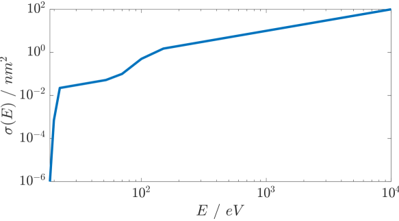
Figure 13: Cross section for MC collisions for parallel energy loss modeling. Threshold energy is $17.5\,$eV, which is subtracted from electron energy in the event of collision.

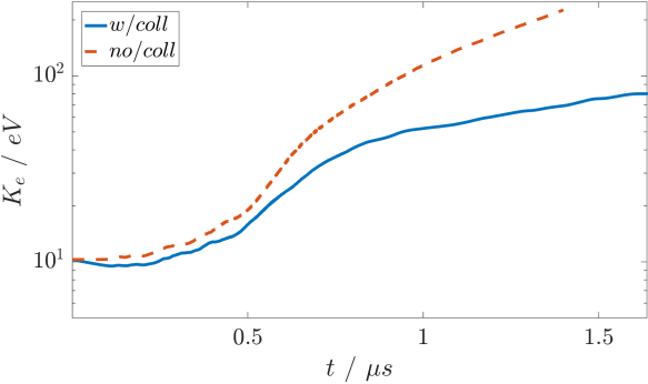
Figure 14: Temperature evolution of electrons with and without collisions.

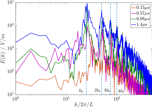
Figure 15: Fluctuation wave number spectrum for the case with electron energy losses.

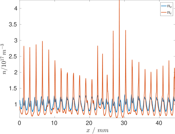
Figure 16: Ion and electron densities when energy loss is introduced for electrons. Ion density fluctuations are increased, compare with figure 3.

VII Summary

We have investigated the dynamics of electron cyclotron drift instability using highly resolved particle-in-cell simulations in 1D3V with realistic mass ratios and using parameters relevant to the Hall-effect thruster. The large simulation box allowed for investigations of large scale nonlinear dynamics of ECDI pumped by transverse $\mathbf{E\times B}$ current. In the nonlinear regime we observe a large amplitude coherent mode (periodic cnoidal wave) driven mainly at the electron cyclotron drift cyclotron resonance $k_{0}=\Omega_{ce}/v_{E}$. High $k$ mode generation occurs due to wave focusing (sharpening) associated with nonlinear ion breaking Davidson (2012), particularly evident in the ion density fluctuations. Simultaneously, we observe energy flow to long wave length and low frequency modes manifested by the generation of the long wavelength envelope. The long wavelength oscillations in our simulations develop on the $\mu$s time scale (or a little faster) and these modes could be similar to the low frequency features that were found in recent experimental observation of the $\mathbf{E\times B}$ instability Tsikata and Minea (2015). The long wavelength modulations in our simulations also resemble some nonlinear features of the electron cyclotron modes observed in Earth’s bow shockBreneman et al. (2013). The generation of the long wavelength mode and associated with it energy transfer to the long wavelength part of the spectrum is expected to be important in the mode saturation mechanism along with possible parametric instabilities of large amplitude waves.Akhiezer, Mikhailenko, and Stepanov (1998); Mikhailenko, Stepanov, and Scime (2003)

We have shown here that demagnetization criterion due to nonlinear resonance broadening (and overlapping) is not fulfilled for electrons in our simulations. The electron cyclotron resonances remain prominently evident, especially at low $m$, while higher resonances become sub-dominant, which is similar to the results of other simulations of electron-cyclotron instability performed for space conditions Muschietti and Lembège (2013, 2006). The full demagnetization of the electron response requires two conditions: $k\rho_{e}\gg 1$ – the modes have to be in the short wavelength regime, and $\Xi k\rho_{e}>1$ – for the nonlinear destruction of the cyclotron resonances. These two conditions (formally equivalent to the limit of zero magnetic field, $B\rightarrow 0))$ result in the fully demagnetized electron response and the resonant drive fully equivalent to that of the beam of unmagnetized electrons. For turbulent fluctuations in our simulations, the condition $k\rho_{e}\gg 1$, is only marginally exceeded, see Fig. 10, while the condition $\Xi k\rho_{e}>1$ is not satisfied, see Fig. 9. This suggests that the magnetic field remains important in the mechanism of the instability, electron heating and transport.

Our simulations show that overall electron dynamics is dominated by the cascade to long wavelength, low frequency modes down to the lower hybrid range and below. An important conclusion from our simulations is that the anomalous electron current is dominated by the contributions from long wavelength (sub-cyclotron-resonance harmonics) modes, from a few mm up to the box size, Fig. 12. This feature is consistent with experimental observations in which a significant fraction of the anomalous current is directed through the large scale spoke structure Parker, Raitses, and Fisch (2010). We speculate that while the energy input via the resonant ECDI may occur at small scales, the nonlinear inverse cascade analogous to our 1D case result in energy condensation in large-scale structures, as also shown by analytical theory in Ref. Lakhin et al., 2016.

Our simulations, while demonstrating important features of the electron cyclotron modes driven by $\mathbf{E\times B}$ current, have certain limitations due to their 1D nature. In general, the fluctuations are expected to have 3D structure as experimental measurements indicate Tsikata et al. (2010). There are several ways in which fluctuations and transport in general 3D case may differ from a simple 1D case.

First, when both components of the fluctuating electric field in the plane perpendicular to the magnetic field are present, one can expect that anomalous contributions both in $\mathbf{E}$ and $\mathbf{E\times B}$ directions will be present (see also the discussion in Section V above) and thus modify the total current in the direction of the applied electric field. The external electric field will have to be determined self-consistently Boeuf (2017) as result of the balance of fluctuation energy (and the resulting anomalous current) and the externally applied potential difference.

Another important point is that fluctuations with a finite value of the wave vector along the magnetic field, $k_{\parallel}$, may have different dispersion properties and instability conditions. As it was shown in Refs. Gary, 1970, 1971; Arefev, 1970, and also more recently in Ref. Cavalier et al., 2013, the short wavelength instabilities with significantly large values of $k_{\parallel}\rho_{e}\geq O(1)$ reduce to the unmagnetized (ion-sound) form. The actual 3D structure of instable modes and its role in the linear and nonlinear development of unstable modes has to be determined in self-consistent simulations resolving the direction along the magnetic field Croes et al. (2017) and proper account of sheath boundary conditions Smolyakov et al. (2013). In our simulations, only an approximate model of parallel losses was used to limit the saturation amplitude for unstable modes. Saturation mechanisms that ultimately will define the mode amplitude are sensitive to the particle and energy losses Boeuf (2014, 2017) including those along the magnetic field as well as ionization effects which are also important for $E\times B$ plasmasEscobar and Ahedo (2014, 2015). Comprehensive account of all these effects also has to be done in full cylindrical geometryCarlsson et al. (2015). However, even in 1D simulations the importance of good resolution and a sufficiently large simulation domain becomes apparent.

In general 2D and 3D cases, the gradient-driven and lower hybrid type instability will be operative Davidson and Krall (1977); Smolyakov et al. (2017); Matsukiyo and Scholer (2006). One can therefore expect that the energy accumulation in long-wavelength modes and contribution to the anomalous transport will be further enhanced by the gradient-drift instabilities which generally have longer wavelengths compared to the cyclotron modes studied here and will be directly active in the mesoscale part of spectrum; between the external scale (of the order of the size of the device) and small scales of the unstable modes.

Part of this picture is the excitation of the gradient driven modes inside large scale structures as seen in as well in PIC simulations that show the $\lambda=4\,$mm wavelength fluctuations inside the spokeMatyash et al. (2013). In our periodic simulations, the external length scale is limited by the simulation box size. In realistic 2D/3D simulations this size can be related to the geometric size, like the lowest $m=1$ mode for cylindrical geometry. Additional processes as energy losses to the wall and ionization will also affect the scale of the large sale structure and reduce the fluctuation amplitude. In our simulations the fluctuation amplitude is of the order of the equilibrium electric field, while the experimental values are much lower. Tsikata et al. (2010).

This work is supported in part by NSERC Canada, and US Air Force Office of Scientific Research FA9550-15-1-0226. Compute/Calcul Canada computational resources were used. We would like thank E. Startsev (PPPL) for fruitful discussions.

References

References

- Buneman (1962) O. Buneman, Journal of Nuclear Energy. Part C, Plasma Physics, Accelerators, Thermonuclear Research 4, 111 (1962).
- Arefev, Gordeev, and Rudakov (1969) V. I. Arefev, A. V. Gordeev, and L. I. Rudakov, Nuclear Fusion S, 143 (1969).
- Wong (1970) H. V. Wong, Physics of Fluids 13, 757 (1970).
- Gary and Sanderson (1970) S. P. Gary and J. J. Sanderson, Journal of Plasma Physics 4, 739 (1970).
- Lashmore-Davies and Martin (1973) C. N. Lashmore-Davies and T. J. Martin, Nuclear Fusion 13, 193 (1973).
- Smolyakov et al. (2017) A. I. Smolyakov, O. Chapurin, W. Frias, O. Koshkarov, I. Romadanov, T. Tang, M. Umansky, Y. Raitses, I. D. Kaganovich, and V. P. Lakhin, Plasma Physics and Controlled Fusion 59, 13 (2017).
- Davidson and Krall (1977) R. C. Davidson and N. A. Krall, Nuclear Fusion 17, 1313 (1977).
- Sizonenko and Stepanov (1967) V. L. Sizonenko and K. N. Stepanov, Nuclear Fusion 7, 131 (1967).
- Wilson et al. (2010) L. B. Wilson, C. A. Cattell, P. J. Kellogg, K. Goetz, K. Kersten, J. C. Kasper, A. Szabo, and M. Wilber, Journal of Geophysical Research: Space Physics 115, A12104 (2010).
- Wilson et al. (2014a) L. B. Wilson, D. G. Sibeck, A. W. Breneman, O. L. Contel, C. Cully, D. L. Turner, V. Angelopoulos, and D. M. Malaspina, Journal of Geophysical Research: Space Physics 119, 6455 (2014a).
- Wilson et al. (2014b) L. B. Wilson, D. G. Sibeck, A. W. Breneman, O. L. Contel, C. Cully, D. L. Turner, V. Angelopoulos, and D. M. Malaspina, Journal of Geophysical Research: Space Physics 119, 6475 (2014b).
- Breneman et al. (2013) A. W. Breneman, C. A. Cattell, K. Kersten, A. Paradise, S. Schreiner, P. J. Kellogg, K. Goetz, and L. B. Wilson, Journal of Geophysical Research: Space Physics 118, 7654 (2013).
- Muschietti and Lembège (2006) L. Muschietti and B. Lembège, Advances in Space Research 37, 483 (2006).
- Muschietti and Lembège (2013) L. Muschietti and B. Lembège, Journal of Geophysical Research: Space Physics 118, 2267 (2013).
- Matsukiyo and Scholer (2006) S. Matsukiyo and M. Scholer, Journal of Geophysical Research: Space Physics 111, A06104 (2006).
- Biskamp and Chodura (1971) D. Biskamp and R. Chodura, Physical Review Letters 27, 1553 (1971).
- Biskamp and Chodura (1972) D. Biskamp and R. Chodura, Nuclear Fusion 12, 485 (1972).
- Biskamp and Chodura (1973) D. Biskamp and R. Chodura, Physics of Fluids 16, 893 (1973).
- Forslund, Morse, and Nielson (1970) D. W. Forslund, R. L. Morse, and C. W. Nielson, Physical Review Letters 25, 1266 (1970).
- Lampe et al. (1971) M. Lampe, W. Manheimer, J. B. McBride, J. H. Orens, R. Shanny, and R. N. Sudan, Physical Review Letters 26, 1221 (1971).
- Lominadze (1972) D. G. Lominadze, Soviet Physics JETP 36, 686 (1972).
- Tsikata and Minea (2015) S. Tsikata and T. Minea, Physical Review Letters 114, 185001 (2015).
- Smirnov, Raitses, and Fisch (2006) A. N. Smirnov, Y. Raitses, and N. J. Fisch, IEEE Transactions on Plasma Science 34, 132 (2006).
- Adam, Heron, and Laval (2004) J. C. Adam, A. Heron, and G. Laval, Physics of Plasmas 11, 295 (2004).
- Boeuf and Chaudhury (2013) J. P. Boeuf and B. Chaudhury, Physical Review Letters 111, 155005 (2013).
- Boeuf (2014) J.-P. Boeuf, Frontiers in Physics 2 (2014).
- Boeuf (2017) J. P. Boeuf, Journal of Applied Physics 121, 24 (2017).
- Lashmore-Davies (1970) C. N. Lashmore-Davies, Journal of Physics Part A, General 3, L40 (1970).
- Arefev (1970) V. I. Arefev, Soviet Physics Technical Physics-USSR 14, 1487 (1970).
- Lampe et al. (1972a) M. Lampe, J. B. McBride, W. Manheimer, R. N. Sudan, R. Shanny, J. H. Orens, and Papadopo.K, Physics of Fluids 15, 662 (1972a).
- Lampe et al. (1972b) M. Lampe, W. Manheimer, J. B. McBride, and J. H. Orens, Physics of Fluids 15, 2356 (1972b).
- Katz et al. (2015) I. Katz, I. G. Mikellides, R. R. Hofer, and A. L. Ortega, 34th International Electric Propulsion Conference , IEPC (2015).
- Cavalier et al. (2013) J. Cavalier, N. Lemoine, G. Bonhomme, S. Tsikata, C. Honore, and D. Gresillon, Physics of Plasmas 20, 082107 (2013).
- Lafleur, Baalrud, and Chabert (2016a) T. Lafleur, S. D. Baalrud, and P. Chabert, Physics of Plasmas 23, 053502 (2016a).
- Lafleur, Baalrud, and Chabert (2016b) T. Lafleur, S. D. Baalrud, and P. Chabert, Physics of Plasmas 23, 053503 (2016b).
- Baranov et al. (1996) V. Baranov, Y. S. Nazarenko, P. V.A., A. I. Vasin, and Y. M. Yashnov, AIAA/ASME/SAE/ASEE Joint Propulsion Conference , AIAA (1996).
- Ducrocq et al. (2006) A. Ducrocq, J. C. Adam, A. Heron, and G. Laval, Physics of Plasmas 13, 102111 (2006).
- Sydorenko (2006) D. Y. Sydorenko, Particle-in-cell simulations of electron dynamics in low pressure discharges with magnetic fields., Ph.D. thesis, University of Saskatchewan (2006).
- Forslund et al. (1972) D. Forslund, C. Nielson, R. Morse, and J. Fu, Physics of Fluids 15, 1303 (1972).
- Mozer and Sundkvist (2013) F. S. Mozer and D. Sundkvist, Journal of Geophysical Research: Space Physics 118, 5415 (2013).
- Davidson (2012) R. Davidson, Methods in Nonlinear Plasma Theory (Academic Press, New York, 2012).
- Pitaevskii (1963) L. P. Pitaevskii, Soviet Physics JETP 17, 658 (1963).
- Huba and Ossakow (1979) J. D. Huba and S. L. Ossakow, Physics of Fluids 22, 1349 (1979).
- Dum and Sudan (1969) C. T. Dum and R. N. Sudan, Physical Review Letters 23, 1149 (1969).
- Langdon (1979) A. B. Langdon, Physics of Fluids 22, 163 (1979).
- Orfanidis (1996) S. Orfanidis, Introduction to Signal Processing, Prentice Hall international editions (Prentice Hall, 1996).
- Kaganovich et al. (2007) I. D. Kaganovich, Y. Raitses, D. Sydorenko, and A. Smolyakov, Physics of Plasmas 14, 057104 (2007).
- Akhiezer, Mikhailenko, and Stepanov (1998) A. I. Akhiezer, V. Mikhailenko, and K. N. Stepanov, Physics Letters A 245, 117 (1998).
- Mikhailenko, Stepanov, and Scime (2003) V. S. Mikhailenko, K. N. Stepanov, and E. E. Scime, Physics of Plasmas 10, 2247 (2003).
- Parker, Raitses, and Fisch (2010) J. B. Parker, Y. Raitses, and N. J. Fisch, Applied Physics Letters 97, 091501 (2010).
- Lakhin et al. (2016) V. P. Lakhin, V. I. Ilgisonis, A. I. Smolyakov, and E. A. Sorokina, Physics of Plasmas 23, 102304 (2016).
- Tsikata et al. (2010) S. Tsikata, C. Honoré, N. Lemoine, and D. M. Grésillon, Physics of Plasmas 17, 112110 (2010).
- Gary (1970) S. P. Gary, Journal of Plasma Physics 4, 753 (1970).
- Gary (1971) S. P. Gary, Journal of Plasma Physics 6, 561 (1971).
- Croes et al. (2017) V. Croes, T. Lafleur, Z. Bonaventura, A. Bourdon, and P. Chabert, Plasma Sources Science & Technology 26, 034001 (2017).
- Smolyakov et al. (2013) A. I. Smolyakov, W. Frias, I. D. Kaganovich, and Y. Raitses, Physical Review Letters 111 (2013).
- Escobar and Ahedo (2014) D. Escobar and E. Ahedo, Physics of Plasmas 21, 043505 (2014).
- Escobar and Ahedo (2015) D. Escobar and E. Ahedo, Physics of Plasmas 22, 102114 (2015).
- Carlsson et al. (2015) J. Carlsson, I. Kaganovich, A. Khrabrov, E. Raitses, and D. Sydorenko, International Electric Propulsion Conference, Hyogo-Kobe, Japan July 4–10, 2015 , IEPC (2015).
- Matyash et al. (2013) K. Matyash, R. Schneider, S. Mazouffre, S. Tsikata, E. Raitses, and A. Diallo, International Electric Propulsion Conference,Washington D.C., USA, IEPC-2013-307 (2013).