Triple collinear emissions in parton showers

Abstract

A framework to include triple collinear splitting functions into parton showers is presented, and the implementation of flavor-changing NLO splitting kernels is discussed as a first application. The correspondence between the Monte-Carlo integration and the analytic computation of NLO DGLAP evolution kernels is made explicit for both timelike and spacelike parton evolution. Numerical simulation results are obtained with two independent implementations of the new algorithm, using the two independent event generation frameworks P YTHIA and S HERPA .

I Introduction

Parton showers solve the leading-order DGLAP equations Gribov and Lipatov (1972); Lipatov (1975); Dokshitzer (1977); Altarelli and Parisi (1977) using Markovian Monte-Carlo algorithms Buckley et al. (2011). As such they work at much lower computational precision than many other calculational tools used in high-energy physics to date Andersen et al. . Due to their importance for both experimental analyses and phenomenological surveys, a limited set of the most important higher-order effects has been included into parton showers over time, such as angular ordering Marchesini and Webber (1988), and soft-gluon enhancement Catani et al. (1991). The numerical size of the remaining theoretical uncertainties is unclear, especially since parton showers are tuned to match the most relevant experimental observables. The net effect of this tuning is that their predictions are most often accurate, yet imprecise, and that the level of imprecision is difficult to quantify numerically. As fully exclusive, high precision simulations are mandatory in order to perform reliable measurements of Standard Model parameters and/or searches for physics beyond the Standard Model, the extension of parton showers to higher formal accuracy would benefit large parts of the high-energy physics community.

The possibility of including next-to-leading order corrections into parton showers has been explored early on Kato and Munehisa (1987, 1989, 1991); Kato et al. (1992) and was revisited recently Hartgring et al. (2013); Li and Skands (2016). NLO splitting functions have been recomputed using a novel regularization scheme Jadach et al. (2011); Gituliar et al. (2014). The dependence of NLO matching terms on the parton-shower evolution scheme has been investigated in detail Jadach et al. (2016). In addition, the first solutions to incorporate effects beyond the leading-color approximation into parton showers have been found Plätzer and Sjödahl (2012); Nagy and Soper (2015), and threshold logarithms have been included in a fully automated approach Nagy and Soper (2016).

In this publication, we construct a framework for the simulation of triple-collinear parton splittings, which contribute to the next-to-leading order corrections to DGLAP evolution Curci et al. (1980); Furmanski and Petronzio (1980); Floratos et al. (1981a, b). Triple-collinear splitting functions have been known since long Catani and Grazzini (2000), but they have not been included into parton showers to date. We start with the simplest case of the flavor-changing splitting kernels. We use these $1\to 3$ kernels to recompute the timelike and spacelike NLO splitting functions $P_{qq^{\prime}}$ in the $\overline{\mathrm{MS}}$ scheme, and we show how the result can be implemented straightforwardly in its differential form in a Markovian Monte-Carlo simulation, such that the integral matches $P_{qq^{\prime}}$ up to momentum conserving effects. Our algorithm depends crucially on the usage of a weighted parton shower, a technique that was presented in Höche et al. (2010); Lönnblad (2012). We see an opportunity to extend our new method to more complicated triple-collinear splitting functions, and to include virtual corrections, such that all NLO kernels may eventually be calculated on-the-fly, similar to the computation of a fixed-order result in the dipole subtraction method Catani and Seymour (1997).

The outline of this publication is as follows: Sec. II highlights the correspondence between the formalisms for parton-shower evolution and DGLAP evolution. The main components of parton-showers are the splitting kernels and the kinematics mapping, which define the probability and kinematics in the transition from an $n$-parton final state to an $n+1$-parton final state. Section III therefore presents the recomputation of the timelike and spacelike NLO splitting kernels $P_{qq^{\prime}}$ and, based on the individual terms identified in the analytical calculation, the construction of a formalism to include $1\to 3$ branchings in the parton shower. We present a validation of our numerical implementation and a test of the numerical impact of $q\to q^{\prime}$ and $q\to\bar{q}$ splittings in Sec. IV. The kinematical mappings introduced to simulate $1\to 3$ splittings are an integral part of the new algorithm, but their presentation is rather technical and has therefore been included in App. A. Section V contains some concluding remarks.

II Parton-shower formalism

Parton showers implement QCD evolution equations, most commonly the DGLAP equation Gribov and Lipatov (1972); Lipatov (1975); Dokshitzer (1977); Altarelli and Parisi (1977), which governs the evolution in the limits of collinear initial- and final-state parton branchings. The main components of a parton-shower are thus the evolution or splitting kernels and the kinematics mapping which defines how an $n$-parton final state transitions to an $n+1$-parton final state. Modern parton showers implement local four-momentum conservation during this transition, which requires the presence of a parton (or a set of partons) that compensate the missing energy when the parton undergoing evolution is taken off its mass shell. Most commonly this so-called recoil partner is identified with the color-connected parton in the large-$N_{c}$ limit. In order to construct a parton shower implementing triple-collinear splitting functions we are thus left with two main tasks: One is to show that such a shower will implement the NLO DGLAP evolution kernels that pertain to the triple-collinear parton branchings. The other is to define kinematics mappings that allow us to generate $1\to 3$ transitions in the presence of a recoil partner. We will address the problem of the connection of the parton-shower formalism to the DGLAP equation in this section, while the definition of the kinematics and a derivation of the related phase-space factorization in $D$ dimensions is presented in App. A. We will make use of both results in Sec. III.

The evolution of parton densities and fragmentation functions in the collinear limit is governed by the DGLAP equations Gribov and Lipatov (1972); Lipatov (1975); Dokshitzer (1977); Altarelli and Parisi (1977). While they are schematically similar for initial and final state, the implementation in parton-shower programs is radically different between the two, owing to the fact that Monte-Carlo simulations are typically performed for inclusive final states. Nevertheless parton showers do solve the DGLAP equations both in timelike and in spacelike evolution. We will start with the evolution equations for the fragmentation functions $D_{a}^{h}(x,Q^{2})$ for parton of type $a$ to fragment into hadron $h$, and we will suppress the index $h$ for brevity,

$$\frac{{\rm d}\,xD_{a}(x,t)}{{\rm d}\ln t}=\sum_{b=q,g}\int_{0}^{1}{\rm d}\tau\int_{0}^{1}{\rm d}z\,\frac{\alpha_{s}}{2\pi}\big{[}zP_{ab}(z)\big{]}_{+}\,\tau D_{b}(\tau,t)\,\delta(x-\tau z)\;.$$ (1)

In this context, $P_{ab}$ are the unregularized DGLAP evolution kernels, which can be expanded into a power series in the strong coupling. The plus prescription can be used to enforce the momentum and flavor sum rules:

$$\big{[}zP_{ab}(z)\big{]}_{+}=\lim\limits_{\varepsilon\to 0}zP_{ab}(z,\varepsilon)\;,$$ (2)

where

$$P_{ab}(z,\varepsilon)=P_{ab}(z)\,\Theta(1-z-\varepsilon)-\delta_{ab}\sum_{c\in\{q,g\}}\frac{\Theta(z-1+\varepsilon)}{\varepsilon}\int_{0}^{1-\varepsilon}{\rm d}\zeta\,\zeta\,P_{ac}(\zeta)\;.$$ (3)

For finite $\varepsilon$, the endpoint subtraction in Eq. (2) can be interpreted as the approximate virtual plus unresolved real corrections, which are included in the parton shower because the Monte-Carlo algorithm naturally implements a unitarity constraint Jadach and Skrzypek (2004). The precise value of $\varepsilon$ in this case is defined in terms of an infrared cutoff on the evolution variable, using four-momentum conservation. For $0<\varepsilon\ll 1$, Eq. (1) changes to

$$\frac{1}{D_{a}(x,t)}\,\frac{{\rm d}D_{a}(x,t)}{{\rm d}\ln t}=-\sum_{c=q,g}\int_{0}^{1-\varepsilon}{\rm d}\zeta\,\zeta\,\frac{\alpha_{s}}{2\pi}P_{ac}(\zeta)\,+\sum_{b=q,g}\int_{x}^{1-\varepsilon}\frac{{\rm d}z}{z}\,\frac{\alpha_{s}}{2\pi}\,P_{ab}(z)\,\frac{D_{b}(x/z,t)}{D_{a}(x,t)}\;.$$ (4)

Using the Sudakov form factor

$$\Delta_{a}(t_{0},t)=\exp\bigg{\{}-\int_{t_{0}}^{t}\frac{{\rm d}\bar{t}}{\bar{t}}\sum_{c=q,g}\int_{0}^{1-\varepsilon}{\rm d}\zeta\,\zeta\,\frac{\alpha_{s}}{2\pi}P_{ac}(\zeta)\bigg{\}}$$ (5)

one can define the generating function for splittings of parton $a$ as

$$\mathcal{D}_{a}(x,t,\mu^{2})=D_{a}(x,t)\Delta_{a}(t,\mu^{2})\;.$$ (6)

Equation (4) can now be written in the simple form

$$\frac{{\rm d}\ln\mathcal{D}_{a}(x,t,\mu^{2})}{{\rm d}\ln t}=\sum_{b=q,g}\int_{x}^{1-\varepsilon}\frac{{\rm d}z}{z}\,\frac{\alpha_{s}}{2\pi}\,P_{ab}(z)\,\frac{D_{b}(x/z,t)}{D_{a}(x,t)}\;.$$ (7)

The generalization to an $n$-parton state, $\vec{a}=\{a_{1},\ldots,a_{n}\}$, with jets and incoming hadrons resolved at scale $t$ can be made in terms of PDFs, $f$, and fragmenting jet functions, $\mathcal{G}$ Procura and Stewart (2010); Jain et al. (2011). We define the generating function for this state as $\mathcal{F}_{\vec{a}}(\vec{x},t,\mu^{2})$. It obeys the evolution equation

$$\begin{split}\frac{{\rm d}\ln\mathcal{F}_{\vec{a}}(\vec{x},t,\mu^{2})}{{\rm d}\ln t}=&\sum_{i\in{\rm IS}}\sum_{b=q,g}\int_{x_{i}}^{1-\varepsilon}\frac{{\rm d}z}{z}\,\frac{\alpha_{s}}{2\pi}\,P_{ba_{i}}(z)\,\frac{f_{b}(x_{i}/z,t)}{f_{a_{i}}(x_{i},t)}\\ &\qquad+\sum_{j\in{\rm FS}}\sum_{b=q,g}\int_{x_{j}}^{1-\varepsilon}\frac{{\rm d}z}{z}\,\frac{\alpha_{s}}{2\pi}\,P_{a_{j}b}(z)\,\frac{\mathcal{G}_{b}(x_{j}/z,t)}{\mathcal{G}_{a_{j}}(x_{j},t)}\;.\end{split}$$ (8)

This equation can be solved using Markovian Monte-Carlo techniques known as parton showers Buckley et al. (2011). In most cases, parton showers implement final-state branchings in unconstrained evolution. Since Eq. (4) also applies to $\mathcal{G}$ Procura and Stewart (2010), we can use Eq. (4) to remove the dependence of $\mathcal{G}$ from Eq. (8), thus leading to the differential branching probability

$$\begin{split}\frac{{\rm d}}{{\rm d}\ln t}\ln\bigg{(}\frac{\mathcal{F}_{\vec{a}}(\vec{x},t,\mu^{2})}{\prod_{j\in\rm FS}\mathcal{G}_{a_{j}}(x_{j},t)}\bigg{)}=&\sum_{i\in{\rm IS}}\sum_{b=q,g}\int_{x_{i}}^{1-\varepsilon}\frac{{\rm d}z}{z}\,\frac{\alpha_{s}}{2\pi}\,P_{ba_{i}}(z)\,\frac{f_{b}(x_{i}/z,t)}{f_{a_{i}}(x_{i},t)}+\sum_{j\in{\rm FS}}\sum_{b=q,g}\int_{0}^{1-\varepsilon}{\rm d}z\,z\,\frac{\alpha_{s}}{2\pi}\,P_{a_{j}b}(z)\;.\end{split}$$ (9)

A direct consequence of this relation is that the Sudakov factor, Eq. (5), must be used in final-state parton showers that implement splitting kernels beyond the leading order, or else the sum rules will be violated Jadach and Skrzypek (2004). However, at leading order the additional factor $\zeta$ in the integral of Eq. (5) can be replaced by a symmetry factor, because the leading-order DGLAP splitting functions, $P_{ab}^{(0)}$, obey the symmetries

$$\begin{split}\sum_{b=q,g}\int_{0}^{1-\varepsilon}{\rm d}z\,z\,P_{qb}^{(0)}(z)=&\int_{\varepsilon}^{1-\varepsilon}{\rm d}z\,P_{qq}^{(0)}(z)+\mathcal{O}(\varepsilon)\;,\\ \sum_{b=q,g}\int_{0}^{1-\varepsilon}{\rm d}z\,z\,P_{gb}^{(0)}(z)=&\int_{\varepsilon}^{1-\varepsilon}{\rm d}z\,\Big{[}\;\frac{1}{2}P_{gg}^{(0)}(z)+n_{f}\,P_{gq}^{(0)}(z)\;\Big{]}+\mathcal{O}(\varepsilon)\;.\end{split}$$ (10)

This relates the branching formalism employed for our new parton shower to the conventional technique for final-state parton evolution Buckley et al. (2011), where the factor $\zeta$ is replaced by $1/2$. The new formalism has a convenient physical interpretation: The factor $\zeta$ identifies the final-state parton undergoing evolution in the same way that the initial-state parton is identified in initial-state evolution. We will make use of this result in Sec. III.3, where we show how to implement the differential form of the integrated splitting kernels computed in Sec. III.1.

III Incorporation of 1$\to$3 branchings

In this section we detail the formalism used to implement triple-collinear splitting functions, both in the spacelike and in the timelike case. The main result is given by Eq. (32), which unsurprisingly bears a remarkable similarity to the formulation of a fixed-order NLO calculation in the subtraction method. Our algorithm must satisfy the constraint that the integral over the splitting function evaluates to the corresponding NLO evolution kernel first computed in Curci et al. (1980); Furmanski and Petronzio (1980); Floratos et al. (1981a, b) and rederived in Heinrich and Kunszt (1998); Ellis and Vogelsang . To verify this, we recompute the flavor-changing timelike and spacelike kernels $P_{qq^{\prime}}$ in Sec. III.1. We then identify the relevant components to be implemented in the Monte-Carlo simulation and comment on the appropriate transformation of the MC integration variables listed in App. A. We also comment on the possibility to extend this method to splitting functions with leading-order contributions and virtual corrections.

In the triple collinear limit of partons $a$, $i$ and $j$, any QCD (associated) matrix element squared factorizes as Catani and Grazzini (2000)

$$|M_{a,i,j,\ldots,k,\ldots}(p_{a},p_{i},p_{j},\ldots)|^{2}=\left(\frac{8\pi\mu^{2\varepsilon}\alpha_{s}}{s_{aij}}\right)^{2}\mathcal{T}^{ss^{\prime}}_{aij,\ldots}(p_{aij},\ldots)\,P^{ss^{\prime}}_{aij}(p_{a},p_{i},p_{j})\;,$$ (11)

where the superscripts denote the spin-dependence of both the splitting function and the reduced matrix element. We will implement the spin-averaged splitting functions, $\langle P_{aij}\rangle(p_{a},p_{i},p_{j})$, together with related counterterms that are identified in Secs. III.2 and III.3. The factor in parentheses in Eq. (11) is common to all terms. The two powers of the strong coupling are both evaluated at the parton-shower evolution variable, $t$. One factor $s_{aij}$ will be combined with the last term in Eqs. (63), (83), (96) and (111), while the other cancels after transformation of the $s_{ai}$ integration using Eqs. (39) and (44). We will comment on this in Sec. III.3.

III.1 Fixed-order calculation

We use the method outlined in Ritzmann and Waalewijn (2014) to compute both the timelike and the spacelike flavor-changing NLO splitting kernels for massless partons

$$\begin{split}P_{qq^{\prime}}^{(T)}(z)=&\;C_{F}T_{R}\left(+(1+z)\log^{2}(z)-\left(\frac{8}{3}z^{2}+9z+5\right)\log(z)+\frac{56}{9}z^{2}+4z-8-\frac{20}{9z}\right)\;,\\ P_{qq^{\prime}}^{(S)}(z)=&\;C_{F}T_{R}\left(-(1+z)\log^{2}(z)-\left(\frac{8}{3}z^{2}+5z+1\right)\log(z)-\frac{56}{9}z^{2}+6z-2+\frac{20}{9z}\right)\;.\end{split}$$ (12)

The timelike splitting functions can be extracted from the term proportional to $\delta(s)$ in the two-loop matching of the fragmenting jet function, $\mathcal{G}$, while the spacelike splitting function is obtained similarly from the $\delta(s)$ term in the matching condition of the beam function. In the timelike case, the matching condition reads

$$\begin{split}\mathcal{G}_{q}^{i(2)}(s,z,\mu)=\mathcal{J}_{qi}^{(2)}(s,z,\mu)+\sum_{j}\int_{z}^{1}\frac{{\rm d}x}{x}\mathcal{J}_{qj}^{(1)}(s,z/x,\mu)D_{j}^{i(1)}(x,\mu)+\delta(s)D_{q}^{i(2)}(z,\mu)\;.\end{split}$$ (13)

The perturbative fragmentation function at $\mathcal{O}(\alpha_{s}^{2})$ is given by

$$\begin{split}&D_{j}^{i(2)}(z,\mu)=\delta_{ij}\delta(1-z)-\frac{\alpha_{s}}{2\pi}\frac{1}{\varepsilon}P_{ji}^{(0)}(z)\\ &\qquad+\left(\frac{\alpha_{s}}{2\pi}\right)^{2}\left[-\frac{1}{2\varepsilon}P_{ji}^{(1)}(z)+\frac{\beta_{0}}{4\varepsilon^{2}}P_{ji}^{(0)}(z)+\frac{1}{2\varepsilon^{2}}\int_{z}^{1}\frac{{\rm d}x}{x}P_{jk}^{(0)}(x)P_{ki}^{(0)}(z/x)\right]\;.\end{split}$$ (14)

In the timelike case we employ the phase-space parametrization of Gehrmann-De Ridder et al. (2004). We factor out the two-particle phase space, the integration over the three-particle invariant $y_{aij}=s_{aij}/q^{2}$ and the corresponding factors $(y_{aij}(1-y_{aij}))^{1-2\varepsilon}$ as well as the integration over one of the light-cone momentum fractions, which is chosen to be $\tilde{z}=s_{ak}/q^{2}/(1-y_{aij})$. We also remove the square of the normalization factor $(4\pi)^{\varepsilon}/(16\pi^{2}\Gamma(1-\varepsilon))\,(q^{2})^{1-\varepsilon}$. The remaining one-emission phase-space integral reads

$$\begin{split}\int{\rm d}\Phi_{+1}^{(F)}=&\;(1-\tilde{z})^{1-2\varepsilon}\tilde{z}^{-\varepsilon}\int_{0}^{1}{\rm d}\tau\,(\tau(1-\tau))^{-\varepsilon}\int_{0}^{1}{\rm d}v\,(v(1-v))^{-\varepsilon}\;\frac{\Omega(1-2\varepsilon)}{\Omega(2-2\varepsilon)}\int_{0}^{1}{\rm d}\chi\,2(4\chi(1-\chi))^{-1/2-\varepsilon}\;,\end{split}$$ (15)

where $\Omega(n)=2\pi^{n/2}/\Gamma(n/2)$. The variables $\tau$ and $v$ are given by the transformation

$$s_{ai}=s_{aij}(1-\tilde{z}_{j})\,v\;,\qquad\tilde{z}_{j}=\frac{s_{jk}/q^{2}}{1-y_{aij}}=(1-\tilde{z})\,\tau\;.$$ (16)

The azimuthal angle integration is parametrized using $\chi$, which is defined as $s_{ij}=s_{ij,-}+\chi(s_{ij,+}-s_{ij,-})\,,$ with $s_{ij,\pm}$ being the two solutions of the quadratic equation $\cos^{2}\phi_{a,i}^{j,k}=1$, cf. Eq. (70) Gehrmann-De Ridder et al. (2004).

We can now integrate the only diagram contributing to the timelike NLO DGLAP kernel, $P_{qq^{\prime}}^{(T)}(\tilde{z})$, which is given by the triple collinear splitting function Catani and Grazzini (2000)

$$P_{qq^{\prime}}^{1\to 3}=\frac{1}{2}C_{F}T_{R}\frac{s_{aij}}{s_{ai}}\left[-\frac{t_{ai,j}^{2}}{s_{ai}s_{aij}}+\frac{4\,\tilde{z}_{j}+(\tilde{z}_{a}-\tilde{z}_{i})^{2}}{\tilde{z}_{a}+\tilde{z}_{i}}+(1-2\varepsilon)\left(\tilde{z}_{a}+\tilde{z}_{i}-\frac{s_{ai}}{s_{aij}}\right)\right]\;,$$ (17)

where $(\tilde{z}_{a}+\tilde{z}_{i})\,t_{ai,j}=2(\tilde{z}_{a}s_{ij}-\tilde{z}_{i}s_{aj})+(\tilde{z}_{a}-\tilde{z}_{i})s_{ai}$. The result is

$$\begin{split}&\frac{1}{C_{F}T_{R}}\int{\rm d}\Phi_{+1}^{(F)}P_{qq^{\prime}}^{1\to 3}=-\frac{1}{\varepsilon}\left(2(1+\tilde{z})\log\tilde{z}+(1-\tilde{z})+\frac{4}{3\tilde{z}}(1-\tilde{z}^{3})\right)\\ &\qquad-4(1+\tilde{z})\Big{(}{\rm Li}_{2}(\tilde{z})-\zeta_{2}\Big{)}+3(1+\tilde{z})\log^{2}\tilde{z}-\frac{16}{3}(1-\tilde{z})+\frac{2}{3\tilde{z}}(1-\tilde{z}^{3})\\ &\qquad+\left(\frac{8}{3\tilde{z}}+\tilde{z}+3\right)\log\tilde{z}+\left(\frac{8}{3\tilde{z}}(1-\tilde{z}^{3})+2(1-\tilde{z})\right)\log(1-\tilde{z})+\mathcal{O}(\varepsilon)\;.\end{split}$$ (18)

Upon including the propagator term from Eq. (11) and the phase-space factor $y_{aij}^{1-2\varepsilon}$, the leading pole will receive an additional factor $-\delta(y_{aij})/2\varepsilon$. The $1/\varepsilon^{2}$ coefficient thus generated is removed by the renormalization of the fragmentation function. As required, it agrees up to a sign with the corresponding second order $1/\varepsilon^{2}$ coefficient in Eq. (14), which we write as

$$\mathcal{P}_{qq^{\prime}}(\tilde{z})=\int_{\tilde{z}}^{1}\frac{{\rm d}x}{x}P_{qg}^{(0)}(x)P_{gq}^{(0)}(z/x)=\,C_{F}T_{R}\left(2(1+\tilde{z})\log\tilde{z}+(1-\tilde{z})+\frac{4}{3\tilde{z}}(1-\tilde{z}^{3})\right)\;.$$ (19)

Equation (13) can now be employed to extract the NLO DGLAP kernel $P_{qq^{\prime}}^{(T)}(z)$ from the finite remainder of Eq. (18). We subtract the corresponding convolution of the one-loop matching coefficient with the one-loop fragmentation function, which is given by

$$\mathcal{I}_{qq^{\prime}}^{(F)}(\tilde{z})=2\int_{\tilde{z}}^{1}\frac{{\rm d}x}{x}C_{F}\left(\frac{1+(1-x)^{2}}{x}\log(x(1-x))+x\right)P_{gq}^{(0)}(\tilde{z}/x)\;.$$ (20)

Using this technique, we finally obtain the result in Eq. (12).

We now proceed to perform the integral over the triple-collinear splitting function in the spacelike case. We use the phase space parametrization in Ellis and Vogelsang . The azimuthal angle integral is most conveniently parametrized using Eq. (68), which gives ${\rm d}\phi_{i,j}^{a,b}={\rm d}(\vec{p}_{i\perp}\vec{p}_{j\perp})/(|\vec{p}_{i\perp}||\vec{p}_{j\perp}|\sin\phi_{i,j}^{a,b})\,,$ with $\vec{p}_{\perp}$ the transverse momenta with respect to the (anti-)collinear directions defined by $p_{a}$ (and $p_{b}$). We can use a transformation identical to the timelike case Gehrmann-De Ridder et al. (2004). We define $s_{ij}=s_{ij,-}+\chi(s_{ij,+}-s_{ij,-})$, where $s_{ij,\pm}$ are the two solutions of the quadratic equation $\cos^{2}\phi_{i,j}^{a,b}=1$. The related angular integral is ${\rm d}\phi_{i,j}^{a,b}(\sin^{2}\phi_{i,j}^{a,b})^{-\varepsilon}=2{\rm d}\chi\,(4\chi(1-\chi))^{-1/2-\varepsilon}\;.$ We remove the normalization factor $(4\pi)^{2\varepsilon}/(16\pi^{2}\Gamma(1-\varepsilon))^{2}\,s_{aij}^{1-2\varepsilon}$. The full phase space relevant to our computation is then given by

$$\int{\rm d}\Phi_{+1}^{(I)}=\tilde{z}^{-1+\varepsilon}\int_{0}^{1}{\rm d}x\,(1-x)^{-\varepsilon}(x-\tilde{z})^{-\varepsilon}\int_{0}^{1}{\rm d}v\,(v(1-v))^{-\varepsilon}\,\frac{\Omega(1-2\varepsilon)}{\Omega(2-2\varepsilon)}\int_{0}^{1}{\rm d}\chi\,2(4\chi(1-\chi))^{-1/2-\varepsilon}\;.$$ (21)

Using Eq. (17) and the crossing relation

$$P_{qq^{\prime}}(\tilde{z}_{1},\tilde{z}_{2},\tilde{z}_{3},s_{12},s_{13},s_{23})=\tilde{z}_{1}\,P_{q^{\prime}q}(1/\tilde{z}_{1},-\tilde{z}_{2}/\tilde{z}_{1},-\tilde{z}_{3}/\tilde{z}_{1},-s_{12},-s_{13},s_{23})\;,$$ (22)

we can integrate the only contribution to the spacelike NLO DGLAP kernel $P_{qq^{\prime}}^{(S)}(z)$. The result can be expressed in terms of Eq. (18) (see also Curci et al. (1980); Dokshitzer et al. (2006))

$$\begin{split}\int{\rm d}\Phi_{+1}^{(I)}\,\tilde{z}P_{q^{\prime}q}^{1\to 3}=\int{\rm d}\Phi_{+1}^{(F)}P_{qq^{\prime}}^{1\to 3}-2\log\tilde{z}\int_{\tilde{z}}^{1}\frac{{\rm d}x}{x}P_{qg}^{(0)}(x)P_{gq}^{(0)}(\tilde{z}/x)+\mathcal{O}(\varepsilon)\;.\end{split}$$ (23)

As in the timelike case, the $1/\varepsilon$ coefficient will eventually be removed by the renormalization of the PDF. It agrees with the corresponding second order $1/\varepsilon^{2}$ coefficient $\mathcal{P}_{qq^{\prime}}(\tilde{z})$ of Eq. (19) and with the corresponding coefficient in the timelike calculation. The finite remainder of Eq. (23) can be employed to extract the NLO DGLAP kernel $P_{qq^{\prime}}^{(S)}(z)$. In order to do so, we must subtract the corresponding convolution of the one-loop matching coefficient with the first-order renormalization term of the PDFs, which is given by

$$\mathcal{I}_{qq^{\prime}}^{(I)}(\tilde{z})=2\int_{\tilde{z}}^{1}\frac{{\rm d}x}{x}T_{R}\Big{(}(1-2x(1-x))\log(1-x)+2x(1-x)\Big{)}P_{qg}^{(0)}(\tilde{z}/x)\;.$$ (24)

Using this technique, we finally obtain the result in Eq. (12).

The above computations allow us to obtain the NLO DGLAP splitting functions using the triple-collinear splitting functions as an input. The drawback of this method is that the calculation must be performed in $D=4-2\varepsilon$ dimensions, and that the cancellation of the singularities occurs between the integrals. In the next section we will therefore construct a local subtraction scheme that allows to cancel singularities at the integrand level and implement the computation in a manner similar to standard subtraction Catani and Seymour (1997), more precisely modified subtraction Frixione and Webber (2002).

III.2 Definition of a local subtraction procedure

We will now proceed to define a scheme for the fully numerical computation of the kernels in Eq. (12). This method allows us to evaluate the integrals leading to Eq. (12) in four dimensions, which in turn allows to use standard Monte-Carlo techniques to evaluate them numerically. Our method can be likened to a standard NLO calculation using modified subtraction techniques Frixione and Webber (2002). In this context, it is crucial that divergences of the triple-collinear splitting functions cancel locally against the subtraction terms. We therefore compute the differential radiation pattern using the triple-collinear splitting functions of Catani and Grazzini (2000), subtracted by the spin-correlated iterated leading-order splitting functions of Somogyi et al. (2005). We then add the finite remainder of the integrated leading-order splitting functions and the renormalization and matching terms as an endpoint contribution. The details of this procedure are described in the following.

Using the phase-space parametrizations in Eqs. (15) and (21) we can compute the integrals of the iterated leading-order splitting kernels corresponding to Eq. (22). This approximate kernel reads

$$\begin{split}\tilde{P}_{qq^{\prime}}^{1\to 3}(\tilde{z}_{a},\tilde{z}_{i},\tilde{z}_{j},s_{ai},s_{aj},s_{ij})=&\;\frac{s_{aij}}{s_{ai}}\,P_{qg}^{(0)}(\tilde{z}_{j})\,P_{gq}^{(0)}\Big{(}\frac{\tilde{z}_{a}}{\tilde{z}_{a}+\tilde{z}_{i}}\Big{)}\\ =&\;C_{F}T_{R}\frac{s_{aij}}{s_{ai}}\left(\frac{1+\tilde{z}_{j}^{2}}{1-\tilde{z}_{j}}-\varepsilon(1-\tilde{z}_{j})\right)\left(1-\frac{2}{1-\varepsilon}\frac{\tilde{z}_{a}\tilde{z}_{i}}{(\tilde{z}_{a}+\tilde{z}_{i})^{2}}\right)\;.\end{split}$$ (25)

Its integrals are given by

$$\begin{split}\mathrm{I}_{qq^{\prime}}^{(F)}(\tilde{z})=&\;\int{\rm d}\Phi_{+1}^{(F)}\tilde{P}_{qq^{\prime}}^{1\to 3}(\tilde{z},\Phi_{+1})\;\,=\int{\rm d}\Phi_{+1}^{(F)}P_{qq^{\prime}}^{1\to 3}(\tilde{z},\Phi_{+1})-\Delta\mathrm{I}_{qq^{\prime}}(\tilde{z})+\mathcal{O}(\varepsilon)\;,\\ \mathrm{I}_{qq^{\prime}}^{(I)}(\tilde{z})=&\;\int{\rm d}\Phi_{+1}^{(I)}\,\tilde{z}\tilde{P}_{q^{\prime}q}^{1\to 3}(1/\tilde{z},\Phi_{+1})=\int{\rm d}\Phi_{+1}^{(I)}\,\tilde{z}P_{q^{\prime}q}^{1\to 3}(1/\tilde{z},\Phi_{+1})-\Delta\mathrm{I}_{qq^{\prime}}(\tilde{z})+\mathcal{O}(\varepsilon)\;,\\ \end{split}$$ (26)

where

$$\Delta\mathrm{I}_{qq^{\prime}}(\tilde{z})=C_{F}T_{R}\Big{(}5(1-\tilde{z})+2(1+\tilde{z})\log\tilde{z}\Big{)}\;.$$ (27)

As required, the $1/\varepsilon$ poles agree with the integrals of the triple-collinear splitting function, Eqs. (18) and (23). The difference in the finite part is identical in the timelike and the spacelike case. This suggest that the approximate kernel, Eq. (25) can be used as a subtraction term for the full triple-collinear splitting kernel, Eq. (22). It is not, however, a local subtraction term, as the $1/\varepsilon$ pole generated by the $v$-integral cancels only after azimuthal integration. In order to construct a local subtraction term, we employ the spin-dependent splitting function, $P_{qg}^{\mu\nu}$, computed in Somogyi et al. (2005), together with the standard spin-dependent LO splitting function, $P_{gq}^{\mu\nu}$

$$\begin{split}P_{qg}^{\mu\nu}(z,k_{\perp})=&\;C_{F}\left[-\frac{2\,z}{1-z}\frac{k_{\perp}^{\mu}k_{\perp}^{\nu}}{k_{\perp}^{2}}+\frac{1-z}{2}\left(-g^{\mu\nu}+\frac{p^{\mu}n^{\nu}+p^{\nu}n^{\mu}}{pn}\right)\right]\;,\\ P_{gq}^{\mu\nu}(z,k_{\perp})=&\;T_{R}\left[-g^{\mu\nu}+4z(1-z)\frac{k_{\perp}^{\mu}k_{\perp}^{\nu}}{k_{\perp}^{2}}\right]\;.\end{split}$$ (28)

Their scalar product generates an additional contribution to Eq. (25), which reads

$$\Delta\tilde{P}_{qq^{\prime}}^{1\to 3}(\tilde{z}_{a},\tilde{z}_{i},\tilde{z}_{j},s_{ai},s_{aj},s_{ij})=C_{F}T_{R}\frac{s_{aij}}{s_{ai}}\frac{4\tilde{z}_{a}\tilde{z}_{i}\tilde{z}_{j}}{(1-\tilde{z}_{j})^{3}}\left(1-2\cos^{2}\phi_{a,j}^{i,k}\right)\;.$$ (29)

The modified approximate kernel exactly cancels the $1/s_{ai}$ poles present in the triple collinear splitting function, such that their difference can be integrated in four dimensions, leading to the expected result

$$\begin{split}\int{\rm d}\Phi_{+1}^{(F)}\left(P_{qq^{\prime}}^{1\to 3}-\tilde{P}_{qq^{\prime}}^{1\to 3}-\Delta\tilde{P}_{qq^{\prime}}^{1\to 3}\right)(\tilde{z},\Phi_{+1})=&\;\Delta\mathrm{I}_{qq^{\prime}}(\tilde{z})\;,\\ \int{\rm d}\Phi_{+1}^{(I)}\,\tilde{z}\left(P_{qq^{\prime}}^{1\to 3}-\tilde{P}_{qq^{\prime}}^{1\to 3}-\Delta\tilde{P}_{qq^{\prime}}^{1\to 3}\right)(\tilde{z},\Phi_{+1})=&\;\Delta\mathrm{I}_{qq^{\prime}}(\tilde{z})\;.\end{split}$$ (30)

We now define the functions

$$\begin{split}\mathrm{R}_{qq^{\prime}}^{(F)}(\tilde{z},\Phi_{+1})=&\;P_{qq^{\prime}}^{1\to 3}(\tilde{z},\Phi_{+1})\;,&\mathrm{S}_{qq^{\prime}}^{(F)}(\tilde{z},\Phi_{+1})=&\;\tilde{P}_{qq^{\prime}}^{1\to 3}(\tilde{z},\Phi_{+1})+\Delta\tilde{P}_{qq^{\prime}}^{1\to 3}(\tilde{z},\Phi_{+1})\;,\\ \mathrm{R}_{qq^{\prime}}^{(I)}(\tilde{z},\Phi_{+1})=&\;\tilde{z}P_{q^{\prime}q}^{1\to 3}(1/\tilde{z},\Phi_{+1})\;,&\mathrm{S}_{qq^{\prime}}^{(I)}(\tilde{z},\Phi_{+1})=&\;\tilde{z}\tilde{P}_{qq^{\prime}}^{1\to 3}(1/\tilde{z},\Phi_{+1})+\tilde{z}\Delta\tilde{P}_{qq^{\prime}}^{1\to 3}(1/\tilde{z},\Phi_{+1})\;.\end{split}$$ (31)

This allows us to write the NLO kernel as

$$P_{qq^{\prime}}^{(T/S)}(\tilde{z})=\Big{(}\mathrm{I}+\frac{1}{\varepsilon}\,\mathcal{P}-\mathcal{I}\Big{)}_{qq^{\prime}}^{(F/I)}(\tilde{z})+\int{\rm d}\Phi_{+1}^{(F/I)}(\mathrm{R}-\mathrm{S})_{qq^{\prime}}^{(F/I)}(\tilde{z},\Phi_{+1})\;.$$ (32)

This equation bears similarity to the definition of standard and hard events in the MC@NLO method Frixione and Webber (2002) without the related shower evolution. However, in our case it is implemented not as a matching coefficient, but in the exponent of the all-orders Sudakov form factor.

In fact, the parton-shower that is added explicitly in MC@NLO is already present in our case, as we also include the leading-order simulation, which schematically generates the additional contributions at $\mathcal{O}(\alpha_{s}^{2})$

$$\begin{split}&\int{\rm d}\Phi_{+1}^{(F)}\tilde{\mathcal{P}}_{qq^{\prime}}^{1\to 3}(\tilde{z},\Phi_{+1})\Big{(}O(\tilde{z},\Phi_{+1})-O(\tilde{z})\Big{)}\;,\\ &\int{\rm d}\Phi_{+1}^{(I)}\,\tilde{z}\tilde{\mathcal{P}}_{qq^{\prime}}^{1\to 3}(1/\tilde{z},\Phi_{+1})\Big{(}O(\tilde{z},\Phi_{+1})-O(\tilde{z})\Big{)}\;.\end{split}$$ (33)

In this equation, $O$ stands for an arbitrary observable, which picks up the real-emission phase-space dependence in the emission term of the parton shower, and the Born phase-space dependence in the corresponding approximate virtual correction implemented through the Sudakov form factor. As in the case of MC@NLO, Eq. (33) provides the necessary counterterms to generate the correct observable dependence on the real-emission phase-space in Eq. (32). This allows to generate events which are distributed according to the fully differential radiation pattern, as given by the triple-collinear splitting function.

In this context it is important to note that our leading-order parton shower does not yet include the spin-correlation term given by Eq. (29). Therefore, the cancellation generated between terms from Eq. (33) and Eq. (32) is non-local in the azimuthal angle. However, this effect will be suppressed in practice, due to the fact that Eq. (33) is large only in the soft region $z_{j}\to 1$, which is most often not resolved in experimental and phenomenological analyses. We will address the implementation of Eq. (29) in the leading-order simulation in a future publication.

The form of Eq. (32) suggests that our method generalizes to the case with Born contribution and virtual corrections, and that the generic structure will be that of a computation using the NLO dipole subtraction method Catani and Seymour (1997), except that the subtraction terms are evaluated in the real-emission phase space, as required for generating parton-shower input configurations in an MC@NLO Frixione and Webber (2002). A complete set of local counterterms for the real-emission contribution could then be obtained from Somogyi et al. (2005).

III.3 Implementation in the parton shower

This section describes the implementation of the local subtraction procedure outlined above into a Monte-Carlo event generator. As opposed to a leading-order simulation, where all splittings have $2\to 3$ kinematics, the new simulation includes an integral over $2\to 4$ configurations, and endpoint contributions arising from $(\mathrm{I}+\mathcal{P}/\varepsilon-\mathcal{I})$. We first explain how the $2\to 4$ branchings are generated and how the integration variables are connected to the kinematic variables introduced in App. A. The generation of endpoint contributions is a simple extension of the generation of $2\to 4$ branchings, and is described later on.

III.3.1 Differential contributions

The splitting kernels that are differential in the $2\to 4$ -particle phase space are defined by the subtracted triple-collinear splitting functions of Catani and Grazzini (2000). As shown in Sec. III.2 we only need their four-dimensional values. There are two independent flavor-changing contributions, which are given by (cf. Eq. (17))

$$\begin{split}&\mathrm{R}_{qq^{\prime}}^{(F)}(\tilde{z}_{a},\tilde{z}_{i},\tilde{z}_{j},s_{ai},s_{aj},s_{ij})=\frac{1}{2}C_{F}T_{R}\frac{s_{aij}}{s_{ai}}\left[-\frac{t_{ai,j}^{2}}{s_{ai}s_{aij}}+\frac{4\,\tilde{z}_{j}+(\tilde{z}_{a}-\tilde{z}_{i})^{2}}{\tilde{z}_{a}+\tilde{z}_{i}}+\left(\tilde{z}_{a}+\tilde{z}_{i}-\frac{s_{ai}}{s_{aij}}\right)\right]\;,\\ &\mathrm{R}_{q\bar{q}}^{(F)}(\tilde{z}_{a},\tilde{z}_{i},\tilde{z}_{j},s_{ai},s_{aj},s_{ij})=P_{qq^{\prime}}^{1\to 3}(\tilde{z}_{a},\tilde{z}_{i},\tilde{z}_{j},s_{ai},s_{aj},s_{ij})\,\\ &\qquad-\frac{1}{N_{C}}C_{F}T_{R}\frac{s_{aij}}{s_{ai}}\bigg{\{}\frac{2s_{ij}}{s_{aij}}+\frac{1+\tilde{z}_{a}^{2}}{1-\tilde{z}_{i}}-\frac{2\tilde{z}_{i}}{1-\tilde{z}_{j}}-\frac{s_{aij}}{s_{aj}}\frac{\tilde{z}_{a}}{2}\frac{1+\tilde{z}_{a}^{2}}{(1-\tilde{z}_{i})(1-\tilde{z}_{j})}\bigg{\}}+(i\leftrightarrow j)\;.\end{split}$$ (34)

Their corresponding local subtraction terms are given by

$$\begin{split}\mathrm{S}_{qq^{\prime}}^{(F)}(\tilde{z}_{a},\tilde{z}_{i},\tilde{z}_{j},s_{ai},s_{aj},s_{ij})=&\;C_{F}T_{R}\frac{s_{aij}}{s_{ai}}\bigg{[}\,\frac{1+\tilde{z}_{j}^{2}}{1-\tilde{z}_{j}}\left(1-\frac{2\tilde{z}_{a}\tilde{z}_{i}}{(\tilde{z}_{a}+\tilde{z}_{i})^{2}}\right)+\frac{4\tilde{z}_{a}\tilde{z}_{i}\tilde{z}_{j}}{(1-\tilde{z}_{j})^{3}}\left(1-2\cos^{2}\phi_{a,j}^{i,k}\right)\bigg{]}\;,\\ \mathrm{S}_{q\bar{q}}^{(F)}(\tilde{z}_{a},\tilde{z}_{i},\tilde{z}_{j},s_{ai},s_{aj},s_{ij})=&\;\mathrm{S}_{qq^{\prime}}^{(F)}(\tilde{z}_{a},\tilde{z}_{i},\tilde{z}_{j},s_{ai},s_{aj},s_{ij})+(i\leftrightarrow j)\;.\end{split}$$ (35)

Note that the subtraction term for $P_{q\bar{q}}$ is the simple sum of two subtraction terms for $P_{qq^{\prime}}$, i.e. the interference contribution on the last line of Eq. (34) does not create a new singularity. The fully differential initial-state $2\to 4$ splitting kernels are defined by crossing (cf. Eq. (31))

$$\begin{split}\mathrm{R}^{(I)}(\tilde{z}_{a},\tilde{z}_{i},\tilde{z}_{j},s_{ai},s_{aj},s_{ij})=&\;\tilde{z}_{a}\mathrm{R}^{(F)}(1/\tilde{z}_{a},-\tilde{z}_{i}/\tilde{z}_{a},-\tilde{z}_{j}/\tilde{z}_{a},-s_{ai},-s_{aj},s_{ij})\;,\\ \mathrm{S}^{(I)}(\tilde{z}_{a},\tilde{z}_{i},\tilde{z}_{j},s_{ai},s_{aj},s_{ij})=&\;\tilde{z}_{a}\mathrm{S}^{(F)}(1/\tilde{z}_{a},-\tilde{z}_{i}/\tilde{z}_{a},-\tilde{z}_{j}/\tilde{z}_{a},-s_{ai},-s_{aj},s_{ij})\;.\end{split}$$ (36)

The kinematics for $2\to 4$ branchings in our parton-shower implementation is described in App. A, and the kinematics for $2\to 3$ branchings can be found in Höche and Prestel (2015). For a numerical implementation of Eqs. (34)-(36) it is important to match the definition of splitting variables in Catani and Grazzini (2000), or else the local cancellation of singularities will fail. We describe in the following how these variables are chosen in practice, based on the phase-space variables in App. A. We note that in our Monte-Carlo implementations all four-momenta of the $2\to 4$ parton final state are known at the time the splitting kernel is evaluated. We could therefore simply use the formal definitions in Catani and Grazzini (2000). However, we find it instructive to write the arguments of the splitting kernels explicitly in terms of the variables used in App. A.

In the case of final-state emitter with final-state spectator, we have the evolution and splitting variables (see App. A.1)

$$t=\frac{4\,p_{j}p_{ai}\,p_{ai}p_{k}}{q^{2}}\;,\quad z_{a}=\frac{2\,p_{a}p_{k}}{q^{2}}\;\qquad\text{and}\qquad s_{ai}\;,\quad x_{a}=\frac{p_{a}p_{k}}{p_{ai}p_{k}}\;.$$ (37)

We can thus identify the variables in Eqs. (34) and (35) as follows

$$\tilde{z}_{a}=\frac{z_{a}}{1-s_{aij}/q^{2}}\;,\qquad\tilde{z}_{i}=\frac{\xi_{a}-z_{a}}{1-s_{aij}/q^{2}}\;,\qquad\tilde{z}_{j}=1-\tilde{z}_{a}-\tilde{z}_{i}\qquad\text{where}\qquad s_{aij}=t/\xi_{a}+s_{ai}\;.\qquad$$ (38)

The scalar products $s_{aj}$ and $s_{ij}$ are computed explicitly. We transform the $s_{ai}$ integration such as to obtain a value in the physical region $s_{ai}\leq s_{aij}$.

$${\rm d}s_{ai}=\frac{{\rm d}\tilde{v}}{1-\tilde{v}}\,s_{aij}\;,\qquad\text{where}\qquad\tilde{v}=\frac{s_{ai}}{s_{aij}}\;.$$ (39)

The factor $s_{aij}$ on the right hand side cancels one of the denominators in the term in parentheses of Eq. (11). In the case of final-state emitter with initial-state spectator, we have the evolution and splitting variables (see App. A.2)

$$t=\frac{2\,p_{j}p_{ai}\,p_{ai}p_{b}}{p_{aij}p_{b}}\;,\quad z_{a}=\frac{p_{a}p_{b}}{p_{aij}p_{b}}\;\qquad\text{and}\qquad s_{ai}\;,\quad x_{a}=\frac{p_{a}p_{b}}{p_{ai}p_{b}}\;$$ (40)

We identify the variables in Eqs. (34) and (35) as follows

$$\tilde{z}_{a}=z_{a}\;,\qquad\tilde{z}_{i}=\xi_{a}-z_{a}\;,\qquad\tilde{z}_{j}=1-\xi_{a}\;.\qquad$$ (41)

The scalar products $s_{aj}$ and $s_{ij}$ are computed explicitly, and the $s_{ai}$ integration is transformed as in Eq. (39). In the case of initial-state emitter with final-state spectator, we have the evolution and splitting variables (see App. A.3)

$$\begin{split}t=\frac{2\,p_{j}p_{ai}\,p_{ai}p_{k}}{p_{a}p_{ijk}}\;,\quad z_{a}=\frac{-q^{2}}{2\,p_{a}p_{ijk}}\qquad\text{and}\qquad s_{ai}\;,\quad x_{a}=\frac{p_{ai}p_{k}}{p_{a}p_{ijk}}\;.\end{split}$$ (42)

We identify the variables in Eqs. (36) as follows

$$\frac{-\tilde{z}_{j}}{\tilde{z}_{a}}=1-\frac{C}{\xi_{a}}\;,\qquad\frac{-\tilde{z}_{i}}{\tilde{z}_{a}}=\frac{2p_{i}p_{k}}{q^{2}/C}\;,\qquad\frac{1}{\tilde{z}_{a}}=1-\tilde{z}_{i}-\tilde{z}_{j}\;,\qquad\text{where}\qquad\frac{1}{C}=1+\frac{t/x_{a}-s_{ai}}{q^{2}}\;.\qquad$$ (43)

The scalar products $s_{aj}$ and $s_{ij}$ are computed explicitly. Using the relation $s_{aij}=-t/x_{a}+s_{ai}+m_{j}^{2}$, we transform the $s_{ai}$ integration such as to obtain a value in the physical region $s_{ai}\leq s_{aij}/\xi_{a}$.

$${\rm d}s_{ai}=\frac{{\rm d}\tilde{v}}{1-\tilde{v}/\xi}\,s_{aij}\;,\qquad\text{where}\qquad\tilde{v}=\xi_{a}\frac{s_{ai}}{s_{aij}}\;.$$ (44)

Note that in this case the $\tilde{v}$ integral is limited to $0<\tilde{v}\leq\xi_{a}$. The factor $s_{aij}$ on the right hand side cancels one of the denominators in the term in parentheses of Eq. (11). In the case of initial-state emitter with initial-state spectator, we have the evolution and splitting variables (see App. A.4)

$$\begin{split}t=\frac{2\,p_{j}p_{ai}\,p_{ai}p_{b}}{p_{a}p_{b}}\;,\quad z_{a}=\frac{q^{2}}{2\,p_{a}p_{b}}\qquad\text{and}\qquad s_{ai}\;,\quad x_{a}=\frac{p_{ai}p_{b}}{p_{a}p_{b}}\;.\end{split}$$ (45)

We identify the variables in Eqs. (36) as follows

$$\frac{1}{\tilde{z}_{a}}=\frac{C}{z_{a}}\;,\qquad\frac{-\tilde{z}_{i}}{\tilde{z}_{a}}=-\frac{1-x_{a}}{z_{a}/C}\;,\qquad\frac{-\tilde{z}_{j}}{\tilde{z}_{a}}=1-\frac{C}{\xi_{a}}\;,\qquad\text{where}\qquad\frac{1}{C}=1+\frac{t/x_{a}-s_{ai}}{q^{2}}\;.\qquad$$ (46)

The scalar products $s_{aj}$ and $s_{ij}$ are computed explicitly, and the $s_{ai}$ integration is transformed as in Eq. (44).

We use the Sudakov veto algorithm to select the evolution variable $t$, based on an overestimate that is given by the soft enhanced term of the leading-order $q\to g$ splitting function. The variable $z_{a}$ is selected accordingly, and the variable $x_{a}$ is generated logarithmically between $z_{a}$ and 1. The variable $v$ is generated uniformly between 0 and 1.

Negative values of the splitting kernels are handled using the weighting technique presented in Höche et al. (2010); Lönnblad (2012). If we assume for the moment that the splitting function is given by $f$, and we use the overestimate $g$, then we can introduce an auxiliary overestimate $h$ which is adjusted such that the probability $f/h$ to accept a splitting conforms to $f/h\in[0,1]$. This implies that $h$ may have a similarly complex functional dependence on the phase-space variables as $f$ itself. The fact that $f/h$ is used as accept probability in the Monte Carlo implementation is corrected by a multiplicative weight, which ensures the proper exponentiation of the desired branching probability.

$$w=\frac{h}{g}\times\begin{cases}~{}\displaystyle\frac{g-f}{h-f}&\quad{\textnormal{if the splitting was rejected,}}\\[8.53581pt] ~{}\displaystyle 1&\quad{\textnormal{if the splitting was accepted.}}\end{cases}$$ (47)

III.3.2 Endpoint contributions

In order to implement Eq.(32) in a parton shower, we find it convenient to perform the integration of $(\mathrm{I}+\mathcal{P}/\varepsilon-\mathcal{I})$ numerically using the method outlined in Sec. II. This will eventually allow us to match the phase-space coverage of the real-correction and the local subtraction terms in the corresponding integrated MC counterterms. Note that the phase-space coverage is restricted in the region $t>0$, as the $z_{a}$ integration range is limited by momentum conservation, cf. Sec. II. This phase-space restriction is the main difference between the algorithm proposed here and the analytic calculation in Sec. III.1. In addition, a fully numerical evaluation of $(\mathrm{I}+\mathcal{P}/\varepsilon-\mathcal{I})$ allows us to extend the calculation to splitting functions that we have not previously computed analytically, such as the flavor-changing contributions $P_{q\bar{q}}$. Note that this kernel in particular does not require any new endpoint contributions beyond those that can be obtained from crossing relations. Thus, the full benefit of our method will become apparent only when implementing the more complicated triple-collinear splitting functions.

The procedure for the MC integration of $(\mathrm{I}+\mathcal{P}/\varepsilon-\mathcal{I})$ is as follows: We generate configurations in the $2\to 4$-parton phase space as described in App. A, which are subsequently projected onto $s_{ai}=0$, while the dependence on $x_{a}$ and $\xi_{a}$ is retained. This corresponds to singling out the pole term in the expansion

$$\frac{1}{v^{1+\varepsilon}}=-\frac{1}{\varepsilon}\,\delta(v)+\sum_{i=0}^{\infty}\frac{\varepsilon^{n}}{n!}\left(\frac{\log^{n}v}{v}\right)_{+}$$ (48)

The $1/\varepsilon$ poles that are generated in this manner will cancel between the integrated subtraction term, $\mathrm{I}$, and the renormalization term, $\mathcal{P}$. In order to compute the finite remainder of $(\mathrm{I}+\mathcal{P}/\varepsilon-\mathcal{I})$, we simply need to implement the $\mathcal{O}(\varepsilon)$ terms in the expansion of the differential forms of the subtraction and matching terms. They are given by

$$\begin{split}\Delta\mathrm{I}_{qq^{\prime}}^{(F)}(\tilde{z}_{a},\tilde{z}_{i},\tilde{z}_{j})=&\;\tilde{\mathrm{I}}_{qq^{\prime}}(\tilde{z}_{a},\tilde{z}_{i},\tilde{z}_{j},\tilde{z}_{a})-\tilde{\mathcal{I}}_{qq^{\prime}}(\tilde{z}_{a},\tilde{z}_{i},\tilde{z}_{j},\tilde{z}_{a}+\tilde{z}_{i})\;,\\ \Delta\mathrm{I}_{qq^{\prime}}^{(I)}(\tilde{z}_{a},\tilde{z}_{i},\tilde{z}_{j})=&\;\tilde{z}_{a}\left[\,\tilde{\mathrm{I}}_{qq^{\prime}}\Big{(}\frac{1}{\tilde{z}_{a}},\frac{-\tilde{z}_{i}}{\tilde{z}_{a}},\frac{-\tilde{z}_{j}}{\tilde{z}_{a}},\frac{\tilde{z}_{a}}{\tilde{z}_{a}+\tilde{z}_{j}}\Big{)}-\tilde{\mathcal{I}}_{qq^{\prime}}\Big{(}\frac{1}{\tilde{z}_{a}},\frac{-\tilde{z}_{i}}{\tilde{z}_{a}},\frac{-\tilde{z}_{j}}{\tilde{z}_{a}},\frac{-\tilde{z}_{a}}{\tilde{z}_{a}+\tilde{z}_{j}}\Big{)}\,\right]\;.\end{split}$$ (49)

where

$$\begin{split}\tilde{\mathrm{I}}_{qq^{\prime}}(\tilde{z}_{a},\tilde{z}_{i},\tilde{z}_{j},\tilde{x})=&\;C_{F}T_{R}\left[\frac{1+\tilde{z}_{j}^{2}}{1-\tilde{z}_{j}}+\left(1-\frac{2\,\tilde{z}_{a}\tilde{z}_{i}}{(\tilde{z}_{a}+\tilde{z}_{i})^{2}}\right)\left(1-\tilde{z}_{j}+\frac{1+\tilde{z}_{j}^{2}}{1-\tilde{z}_{j}}\right)\Big{(}\log(\tilde{x}\,\tilde{z}_{i}\tilde{z}_{j})-1\Big{)}\right]\;,\\ \tilde{\mathcal{I}}_{qq^{\prime}}(\tilde{z}_{a},\tilde{z}_{i},\tilde{z}_{j},\tilde{x})=&\;2C_{F}\left[\,\frac{1+\tilde{z}_{j}^{2}}{1-\tilde{z}_{j}}\log(\tilde{x}\,\tilde{z}_{j})+(1-\tilde{z}_{j})\,\right]P_{gq}^{(0)}\Big{(}\frac{\tilde{z}_{a}}{\tilde{z}_{a}+\tilde{z}_{i}}\Big{)}\;.\end{split}$$ (50)

The endpoint contributions for $q\to\bar{q}$ transitions are obtained as a sum of two terms of $q\to q^{\prime}$ type

$$\Delta\mathrm{I}_{q\bar{q}}(\tilde{z}_{a},\tilde{z}_{i},\tilde{z}_{j})=\Delta\mathrm{I}_{qq^{\prime}}(\tilde{z}_{a},\tilde{z}_{i},\tilde{z}_{j})+(i\leftrightarrow j)\;.$$ (51)

III.3.3 Symmetry factors

Finally, according to Sec. II, we multiply each term in Eq. (32) by an additional factor $z_{a}$ in branchings with final-state emitter, independent of the type of spectator. This can be interpreted as an identification of the parton for which the evolution equation is constructed. The extension to $1\to 3$ splittings requires a similar factor for one of the two radiated partons, if the two are indistinguishable. In the case of the simulation presented here this applies to the flavor-changing splittings of type $q\to\bar{q}$. The corresponding extension of the symmetry relation, Eq. (10), reads

$$\begin{split}&\sum_{b=q,g}\int_{0}^{1-\varepsilon}{\rm d}z_{1}\int_{0}^{1-\varepsilon}{\rm d}z_{2}\,\frac{z_{1}\,z_{2}}{1-z_{1}}\,\Theta(1-z_{1}-z_{2})\,P_{a\to ab\bar{b}}(z_{1},z_{2},\ldots)\\ &\qquad=\sum_{b=q,g}\int_{\varepsilon}^{1-\varepsilon}{\rm d}z_{1}\,\int_{\varepsilon}^{1-z_{1}}{\rm d}z_{2}\,S_{ab\bar{b}}\,P_{a\to ab\bar{b}}(z_{1},z_{2},\ldots)+\mathcal{O}(\varepsilon)\;,\\ &\sum_{\begin{subarray}{c}b=q,g\\ b\neq a\end{subarray}}\int_{0}^{1-\varepsilon}{\rm d}z_{1}\int_{0}^{1-\varepsilon}{\rm d}z_{2}\,\frac{z_{1}\,z_{2}}{1-z_{1}}\,\Theta(1-z_{1}-z_{2})\,\Big{(}P_{a\to ba\bar{b}}(z_{1},z_{2},\ldots)+P_{a\to b\bar{b}a}(z_{1},z_{2},\ldots)\Big{)}\\ &\qquad=\sum_{\begin{subarray}{c}b=q,g\\ b\neq a\end{subarray}}\int_{\varepsilon}^{1-\varepsilon}{\rm d}z_{1}\,\int_{\varepsilon}^{1-z_{1}}{\rm d}z_{2}\,S_{ab\bar{b}}\,P_{a\to ba\bar{b}}(z_{1},z_{2},\ldots)+\mathcal{O}(\varepsilon)\;,\end{split}$$ (52)

where $S_{ab\bar{b}}=1/(\prod_{c=q,g}n_{c}!)$, with $n_{c}$ the number of partons of type $c$, is the usual symmetry factor for the final-state $ab\bar{b}$. Thus, all terms in Eq. (32) are multiplied by the following overall symmetry factors:

$$\begin{split}S^{(F)}=&\;z_{a}\,\frac{\xi_{a}-z_{a}}{1-z_{a}}\;,\qquad&S^{(I)}=&\;\frac{1-x_{a}}{1-z_{a}}\;.\end{split}$$ (53)

IV Numerical results

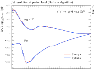
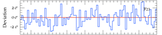
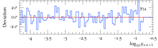
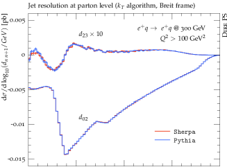
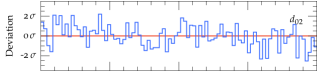
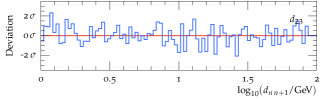
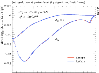
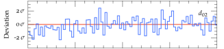
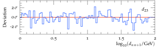
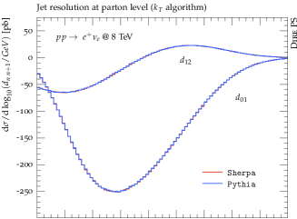
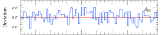
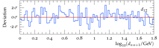
Figure 1: Validation of the simulation of triple-collinear parton splittings in final-state (top row) and initial-state (bottom row) branchings with final-state (left panels) and initial-state (right panels) spectator. We show Durham $k_{T}$-jet rates in $e^{+}e^{-}\to$hadrons at LEP I, $k_{T}$-jet rates in neutral current DIS at HERA II with $Q^{2}>100~{}{\rm GeV}^{2}$, and $k_{T}$-jet rates in $pp\to e^{+}\nu_{e}$ at the 8 TeV LHC (top left to bottom right).

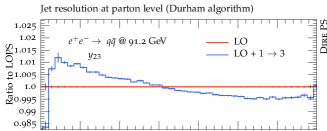
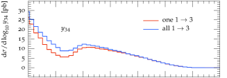
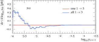
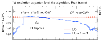
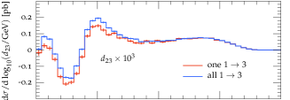
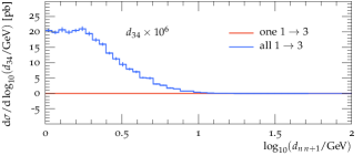
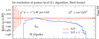
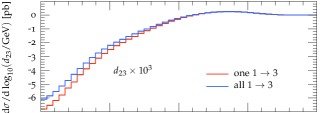
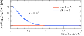
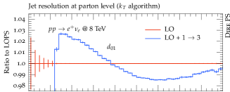
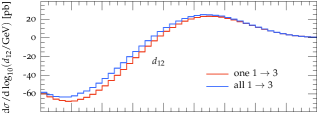
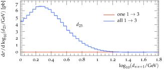
Figure 2: Impact of the simulation of triple-collinear parton splittings on final-state (top row) and initial-state (bottom row) evolution with final-state (left panels) and initial-state (right panels) spectator. Top panels show the ratio between the leading-order result and the leading-order simulation including triple-collinear branchings. Middle and bottom panels show a comparison between the simulation of up to one triple-collinear splitting and arbitrarily many (both not including the leading-order result). For details, see Fig. 1.

In this section we present numerical cross-checks of our algorithm, and we compare the magnitude of the corrections generated by the flavor-changing triple-collinear splitting functions to the leading-order parton-shower result. We have implemented our algorithm into the D IRE parton showers, which implies two entirely independent realizations within the general purpose event generation frameworks P YTHIA  Sjöstrand (1985); Sjöstrand et al. (2015) and S HERPA  Gleisberg et al. (2004, 2009). We employ the CT10nlo PDF set Lai et al. (2010), and use the corresponding form of the strong coupling. Following standard practice to improve the logarithmic accuracy of the parton shower, the soft enhanced term of the leading-order splitting functions is rescaled by $1+\alpha_{s}(t)/(2\pi)K$, where $K=(67/18-\pi^{2}/6)\,C_{A}-10/9\,T_{R}\,n_{f}$ Catani et al. (1991).

Figure 1 shows comparisons between the results from D IRE +P YTHIA and D IRE +S HERPA for a single triple collinear splitting. Each simulation contains $10^{9}$ events. The lower panels present the deviation between the two predictions, normalized to the statistical uncertainty of D IRE +S HERPA in the respective bin. If both implementations are equivalent, this distribution should exhibit statistical fluctuations only. We validate final-state emissions with final-state spectator in the reaction $e^{+}e^{-}\to\text{hadrons}$ (Fig. 1), final-state emissions with initial-state spectator and initial-state emissions with final-state spectator in the reaction $e^{+}p\to e^{+}\text{jet}$ (Figs. 1 and 1), and initial-state emissions with initial-state spectator in the reaction $pp\to e^{+}\nu_{e}$ (Fig. 1). As required, the two implementations agree perfectly. Each panel shows the predictions for the leading two differential jet rates, which are both populated by the simulation of a single triple collinear parton branching. Note that their numerical values can be both positive and negative, since the triple collinear splitting functions are not positive-definite. While the sub-leading jet rate receives contributions from the simulation of $\mathrm{R}-\mathrm{S}$ in Eq. (32) only, the leading jet rate also receives contributions from $\mathrm{I}-\mathcal{I}$. It can be seen that in all cases $\mathrm{I}-\mathcal{I}$ is much large on average than $\mathrm{R}-\mathrm{S}$. The feature around -2.5 in Fig. 1 and around 0.7 in Fig. 1 is due to the onset of $b$-quark production, which we include in the simulation only if $t>m_{b}^{2}$. Similar, yet less pronounced, features are present in Figs. 1 and 1.

Figure 2 shows the impact of triple-collinear parton branchings on the full evolution. We compare the ratio of leading-jet rates with and without the simulation of $1\to 3$ splittings (upper panels), and we analyze the impact of multiple $1\to 3$ splittings compared to a single one (middle and lower panels). The edge in the ratio plots is related to the parton-shower cutoff, where the $1\to 3$ splittings have a different behavior compared to the leading-order ones due to the different evolution variable. It is apparent that the effect of multiple triple-collinear branchings is marginal, even more so when compared to the leading-order results, which are by themselves much larger in magnitude than the correction from a single $1\to 3$ branching. We note again that the largest part of the $1\to 3$ results is due to the subtraction terms $\mathcal{I}_{qq^{\prime}}$, which is in fact a leading-order like contribution. The impact of the $1\to 3$ flavor-changing splittings is particularly small for $e^{+}e^{-}\to\text{hadrons}$. For $e^{+}p\to e^{+}\text{jet}$ scatterings, the hard-emission regions show the largest impact, while for $pp\to e^{+}\nu_{e}$, the soft- and collinear-emission regions are enhanced.

V Conclusions

We have presented a new scheme to include triple collinear splitting functions into parton showers. As a proof of principle we have recomputed the timelike and spacelike flavor-changing NLO DGLAP kernels $P_{qq^{\prime}}$ and matched each component of the integrand to the relevant parton-shower expression. The implementation into two entirely independent Monte-Carlo simulations, based on the general-purpose event generation frameworks P YTHIA and S HERPA has been cross-checked to very high numerical accuracy. The impact of the flavor changing triple-collinear kernels $P_{qq^{\prime}}$ and $P_{q\bar{q}}$ has been studied in timelike and spacelike parton evolution as a first application. We find that the numerical impact of the kernels investigated here is marginal, with effects of up to $\sim 1$% on differential jet rates in $e^{+}e^{-}\to$hadrons at $\sqrt{s}$=91.2 GeV (LEP I), neutral-current DIS with $Q^{2}>100$ GeV² at $\sqrt{s}$=300 GeV (HERA II), and $pp\to e^{+}\nu_{e}$ at 8 TeV (LHC I).

Appendix A Kinematics and phase-space factorization for $1\to 3$ splittings

In this section we give the phase-space parametrizations employed in our implementation of $1\to 3$ parton branchings. We construct kinematic mappings that allow us to relate the splitting and evolution variables to manifestly Lorentz invariant quantities. In order to cover all possible applications, we list formulae for arbitrary external particle masses. While this is not strictly needed in the course of this work, it may be useful to include higher-order effects involving heavy quark splitting functions in the future. The main results are Eqs. (63), (83), (96) and (111), as well as the corresponding $D$-dimensional phase-space factors, Eqs. (74) and (101).

A.1 Final-state emitter with final-state spectator

The kinematics for the case of a final-state radiator with final-state spectator are derived from an iteration of the massive dipole kinematics in Catani et al. (2002). This is sketched in Fig. 3. The evolution and splitting variables are defined as

$$t=\frac{4\,p_{j}p_{ai}\,p_{ai}p_{k}}{q^{2}-m_{aij}^{2}-m_{k}^{2}}\;,\quad z_{a}=\frac{2\,p_{a}p_{k}}{q^{2}-m_{aij}^{2}-m_{k}^{2}}\;\qquad\text{and}\qquad s_{ai}\;,\quad x_{a}=\frac{p_{a}p_{k}}{p_{ai}p_{k}}\;.$$ (54)

We generate the first branching $(\widetilde{a\imath\jmath},\tilde{k})\to(ai,j,k)$ with the mass of the pseudoparticle $ai$ set to the virtuality $s_{ai}$. The new momentum of the spectator parton $k$ is determined as

$$\begin{split}p_{k}^{\,\mu}=&\;\left(\tilde{p}_{k}^{\,\mu}-\frac{q\cdot\tilde{p}_{k}}{q^{2}}\,q^{\mu}\right)\,\sqrt{\frac{\lambda(q^{2},s_{aij},m_{k}^{2})}{\lambda(q^{2},m_{aij}^{2},m_{k}^{2})}}+\frac{q^{2}+m_{k}^{2}-s_{aij}}{2\,q^{2}}\,q^{\mu}\;,\end{split}$$ (55)

with $q=\tilde{p}_{aij}+\tilde{p}_{k}$ and $\lambda$ denoting the Källen function $\lambda(a,b,c)=(a-b-c)^{2}-4\,bc$. $s_{aij}$ is given in terms of the evolution and splitting variables as $s_{aij}=y\,(q^{2}-m_{k}^{2})+(1-y)\,(s_{ai}+m_{j}^{2})$, where

$$y=\frac{t\,x_{a}/z_{a}}{q^{2}-s_{ai}-m_{j}^{2}-m_{k}^{2}}\;,\qquad\tilde{z}=\frac{z_{a}/x_{a}}{1-y}\,\frac{q^{2}-m_{aij}^{2}-m_{k}^{2}}{q^{2}-s_{ai}-m_{j}^{2}-m_{k}^{2}}\;.$$ (56)

The new momentum of the emitter parton, $p_{ai}$, is constructed as

$$p_{ai}^{\mu}\,= \;\bar{z}_{ai}\,\frac{\gamma(q^{2},s_{aij},m_{k}^{2})\,p_{aij}^{\mu}-s_{aij}\,p_{k}^{\mu}}{\beta(q^{2},s_{aij},m_{k}^{2})}+\frac{s_{ai}+{\rm k}_{\perp}^{2}}{\bar{z}_{ai}}\,\frac{p_{k}^{\mu}-m_{k}^{2}/\gamma(q^{2},s_{aij},m_{k}^{2})\,p_{aij}^{\mu}}{\beta(q^{2},s_{aij},m_{k}^{2})}+k_{\perp}^{\mu}\;,$$ (57)

where $\beta(a,b,c)={\rm sgn}(a-b-c)\sqrt{\lambda(a,b,c)}$, $2\,\gamma(a,b,c)=(a-b-c)+\beta(a,b,c)$ and $p_{aij}^{\mu}=q^{\mu}-p_{k}^{\mu}$. The parameters $\bar{z}_{ai}$ and ${\rm k}_{\perp}^{2}=-k_{\perp}^{2}$ of this decomposition are given by

$$\begin{split}\bar{z}_{ai}\,=&\;\frac{q^{2}-s_{aij}-m_{k}^{2}}{\beta(q^{2},s_{aij},m_{k}^{2})}\,\left[\;\tilde{z}\,-\,\frac{m_{k}^{2}}{\gamma(q^{2},s_{aij},m_{k}^{2})}\frac{s_{aij}+s_{ai}-m_{j}^{2}}{q^{2}-s_{aij}-m_{k}^{2}}\right]\;,\\ {\rm k}_{\perp}^{2}\,=&\;\bar{z}_{ai}\,(1-\bar{z}_{ai})\,s_{aij}-(1-\bar{z}_{ai})\,s_{ai}-\bar{z}_{ai}\,m_{j}^{2}\;,\end{split}$$ (58)

The transverse momentum is constructed using an azimuthal angle, $\phi_{ai}$

$$k_{\perp}^{\mu}={\rm k}_{\perp}\left(\cos\phi_{ai}\frac{n_{\perp}^{\mu}}{|n_{\perp}|}+\sin\phi_{ai}\frac{l_{\perp}^{\,\mu}}{|l_{\perp}|}\right)\;,\qquad\text{where}\qquad n_{\perp}^{\mu}=\varepsilon^{0\mu}_{\;\;\;\nu\rho}\,\tilde{p}_{aij}^{\,\nu}\,\tilde{p}_{k}^{\,\rho}\;,\qquad l_{\perp}^{\,\mu}=\varepsilon^{\mu}_{\;\nu\rho\sigma}\,\tilde{p}_{aij}^{\,\nu}\,\tilde{p}_{k}^{\,\rho}\,n_{\perp}^{\sigma}\;.$$ (59)

In kinematical configurations where $\vec{\tilde{p}}_{aij}=\pm\vec{\tilde{p}}_{k}$, $n_{\perp}$ in the definition of Eq. (59) vanishes. It can then be computed as $n_{\perp}^{\mu}=\varepsilon^{0\,i\mu}_{\;\;\;\;\;\nu}\,\tilde{p}_{aij}^{\,\nu}$, where $i$ may be any index that yields a nonzero result.

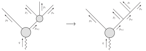
Figure 3: Kinematics mapping for final-state splittings with final-state spectator.

The first branching step, which generates the final-state momentum $p_{j}$ and the intermediate momentum $p_{ai}$ is followed by a second step, constructed using the same algorithm. As $p_{ai}$ has been generated with virtuality $s_{ai}$, no momentum reshuffling is necessary in this case, and $p_{k}$ serves as the defining vector for the anti-collinear direction only. The customary variables $y$ and $\tilde{z}$ are determined by

$$y^{\prime}=\left[\,1+\frac{z_{a}}{x_{a}}\,\frac{q^{2}-m_{aij}^{2}-m_{k}^{2}}{s_{ai}-m_{a}^{2}-m_{i}^{2}}\right]^{-1}\;,\quad\tilde{z}^{\prime}=x_{a}\;.$$ (60)

Equations (57) and (58) are employed to construct the momenta $p_{a}$ and $p_{j}$ using the replacements $q^{2}\to(p_{ai}+p_{k})^{2}$, $s_{aij}\to s_{ai}$, $s_{ai}\to m_{a}^{2}$ and $m_{j}^{2}\to m_{i}^{2}$.

The phase-space factorization for final-state splittings with final-state spectator can be derived similarly to the $2\to 3$ case described in Dittmaier (2000), App. B. We perform an s-channel factorization over $p_{aij}$ and subsequently over $p_{ai}$. This gives

$$\begin{split}\int{\rm d}\Phi(p_{a},p_{i},p_{j},p_{k}|\,q)=&\int\frac{{\rm d}s_{aij}}{2\pi}\,\int{\rm d}\Phi(p_{aij},p_{k}|\,q)\,\int{\rm d}\Phi(p_{a},p_{i},p_{j}|\,p_{aij})\\ =&\int\frac{{\rm d}s_{aij}}{2\pi}\,\sqrt{\frac{\lambda(q^{2},s_{aij},m_{k}^{2})}{\lambda(q^{2},m_{aij}^{2},m_{k}^{2})}}\int{\rm d}\Phi(\tilde{p}_{aij},\tilde{p}_{k}|\,q)\,\int{\rm d}\Phi(p_{a},p_{i},p_{j}|\,p_{aij})\\ =&\int{\rm d}\Phi(\tilde{p}_{aij},\tilde{p}_{k}|\,q)\,\int\Big{[}{\rm d}\Phi(p_{a},p_{i},p_{j}|\,\tilde{p}_{aij},\tilde{p}_{k})\Big{]}\end{split}$$ (61)

We define the auxiliary variable $\xi_{a}=z_{a}/x_{a}$ and use the relations $z_{a}=(s_{ak}-m_{a}^{2}-m_{k}^{2})/(q^{2}-m_{aij}^{2}-m_{k}^{2})$, $\xi_{a}=(s_{aik}-s_{ai}-m_{k}^{2})/(q^{2}-m_{aij}^{2}-m_{k}^{2})$ and $t=\xi_{a}\,(s_{aij}-s_{ai}-m_{j}^{2})$ to write

$$\begin{split}\int\Big{[}{\rm d}\Phi(p_{a},p_{i},p_{j}|\,\tilde{p}_{aij},\tilde{p}_{k})\Big{]}=&\int\frac{{\rm d}s_{aij}}{2\pi}\,\sqrt{\frac{\lambda(q^{2},s_{aij},m_{k}^{2})}{\lambda(q^{2},m_{aij}^{2},m_{k}^{2})}}\int\frac{{\rm d}s_{ai}}{2\pi}\int{\rm d}\Phi(p_{ai},p_{j}|p_{aij})\int{\rm d}\Phi(p_{a},p_{i}|p_{ai})\\ =&\int\frac{{\rm d}s_{aij}}{2\pi}\,\frac{1}{\sqrt{\lambda(q^{2},m_{aij}^{2},m_{k}^{2})}}\int\frac{{\rm d}s_{ai}}{2\pi}\int\frac{{\rm d}s_{aik}\,{\rm d}\phi_{ai}}{4(2\pi)^{2}}\int\frac{1}{4(2\pi)^{2}}\frac{{\rm d}s_{ak}\,{\rm d}\phi_{a}}{\sqrt{\lambda(s_{aik},s_{ai},m_{k}^{2})}}\\ =&\frac{1}{4(2\pi)^{3}}\frac{q^{2}-m_{aij}^{2}-m_{k}^{2}}{\sqrt{\lambda(q^{2},m_{aij}^{2},m_{k}^{2})}}\int{\rm d}t\int{\rm d}z_{a}\int{\rm d}\phi_{a}\\ &\qquad\times\frac{1}{4(2\pi)^{3}}\int{\rm d}s_{ai}\int\frac{{\rm d}\xi_{a}}{\xi_{a}}\int{\rm d}\phi_{ai}\,\frac{q^{2}-m_{aij}^{2}-m_{k}^{2}}{\sqrt{\lambda(s_{aik},s_{ai},m_{k}^{2})}}\;.\end{split}$$ (62)

The final result is

$$\begin{split}\int\Big{[}{\rm d}\Phi(p_{a},p_{i},p_{j}|\,\tilde{p}_{aij},\tilde{p}_{k})\Big{]}=&\,\frac{J^{(1)}_{\rm FF}}{16\pi^{2}}\int\frac{{\rm d}t}{t}\int{\rm d}z_{a}\int\frac{{\rm d}\phi_{j}}{2\pi}\,\bigg{[}\,\frac{1}{16\pi^{2}}\int{\rm d}s_{ai}\int\frac{{\rm d}\xi_{a}}{\xi_{a}}\int\frac{{\rm d}\phi_{i}}{2\pi}\,J^{(2)}_{\rm FF}\,\bigg{]}\,\frac{t}{\xi_{a}}\;,\end{split}$$ (63)

where we have defined the Jacobian factors

$$J^{(1)}_{\rm FF}=\frac{q^{2}-m_{aij}^{2}-m_{k}^{2}}{\sqrt{\lambda(q^{2},m_{aij}^{2},m_{k}^{2})}}\qquad\text{and}\qquad J^{(2)}_{\rm FF}=\frac{s_{aik}-s_{ai}-m_{k}^{2}}{\sqrt{\lambda(s_{aik},s_{ai},m_{k}^{2})}}\;.$$ (64)

The extension of Eq. (63) to $D=4-2\varepsilon$ dimensions is straightforward. We obtain an additional factor of

$$\tilde{\Delta}\Phi_{\rm FF}(p_{a},p_{i},p_{j}|\,\tilde{p}_{aij},\tilde{p}_{k})=\left(\frac{\lambda(q^{2},s_{aij},m_{k}^{2})}{\lambda(q^{2},m_{aij}^{2},m_{k}^{2})}\right)^{-\varepsilon}\Delta\Phi_{\rm FF}(p_{a},p_{i},p_{j}|\,\tilde{p}_{aij},\tilde{p}_{k})\;,$$ (65)

where

$$\Delta\Phi_{\rm FF}(p_{a},p_{i},p_{j}|\,\tilde{p}_{aij},\tilde{p}_{k})=\left(\frac{\Omega(1-2\varepsilon)}{(2\pi)^{-2\varepsilon}}\right)^{2}\left(\bar{p}_{ai,j}^{2}\sin^{2}\theta_{ai,j}^{\,k}\sin^{2}\phi_{j}\right)^{-\varepsilon}\left(\bar{p}_{a,i}^{2}\sin^{2}\theta_{a,i}^{\,k}\sin^{2}\phi_{i}\right)^{-\varepsilon}\;.$$ (66)

The $n$-dimensional sphere is defined as $\Omega(n)=2\pi^{n/2}/\,\Gamma(n/2)$. We can write the magnitudes of the momenta as

$$\bar{p}_{a,i}^{2}=\frac{\lambda(s_{ai},m_{a}^{2},m_{i}^{2})}{4\,s_{ai}}\;.$$ (67)

The polar angles are given by

$$\cos\theta_{a,i}^{\,k}=-\frac{(s_{ai}+m_{a}^{2}-m_{i}^{2})(s_{ai}+m_{k}^{2}-s_{aik})}{\sqrt{\lambda(s_{ai},m_{a}^{2},m_{i}^{2})\lambda(s_{ai},m_{k}^{2},s_{aik})}}\left(1-\frac{2\,s_{ai}}{s_{ai}+m_{a}^{2}-m_{i}^{2}}\frac{p_{a}p_{k}}{p_{ai}p_{k}}\right)\;.$$ (68)

The splitting functions in our algorithm are independent of $\phi_{j}$, hence we can average over one azimuthal angle, leading to the familiar volume factor

$$\frac{\Omega(2-2\varepsilon)}{(2\pi)^{1-2\varepsilon}}=\frac{\Omega(1-2\varepsilon)}{(2\pi)^{-2\varepsilon}}\int_{0}^{\pi}\frac{{\rm d}\phi_{j}}{2\pi}(\sin^{2}\phi_{j})^{-\varepsilon}=\frac{(4\,\pi)^{\varepsilon}}{\Gamma(1-\varepsilon)}\;.$$ (69)

The azimuthal angle $\phi_{i}$ is parametrized as $\phi_{i}=\phi_{a,j}^{ai,k}$, where

$$\cos\phi_{i,j}^{a,b}=\frac{\bar{s}_{ab}(\bar{s}_{ia}\bar{s}_{jb}+\bar{s}_{ib}\bar{s}_{ja}-\bar{s}_{ij}\bar{s}_{ab})-(s_{a}\bar{s}_{ib}\bar{s}_{jb}+s_{b}\bar{s}_{ia}\bar{s}_{ja}-\bar{s}_{ij}s_{a}s_{b})}{\sqrt{k_{\perp}^{2}(p_{i}|\,p_{a},p_{b})\,k_{\perp}^{2}(p_{j}|\,p_{a},p_{b})}\;\lambda(s_{ab},s_{a},s_{b})/4}\;.$$ (70)

Note that we have defined $\bar{s}_{ij}=p_{i}p_{j}$ to simplify the notation. The transverse momentum squared is given by

$$k_{\perp}^{2}(p_{i}|p_{a},p_{b})=\frac{2\bar{s}_{ab}\bar{s}_{ia}\bar{s}_{ib}-s_{a}\bar{s}_{ib}^{2}-s_{b}\bar{s}_{ia}^{2}-s_{i}\bar{s}_{ab}^{2}+s_{i}s_{a}s_{b}}{\lambda(s_{ab},s_{a},s_{b})/4}\;.$$ (71)

For massless partons, Eq. (68) can be written in the simple form

$$\cos\theta_{a,i}^{k}=1-2\,x_{a}\;,\qquad\cos\theta_{ai,j}^{k}=\frac{s_{aij}+s_{ai}}{s_{aij}-s_{ai}}\left[\,1-2\,\xi_{a}\,\frac{s_{aij}}{s_{aij}+s_{ai}}\,\frac{q^{2}}{q^{2}-s_{aij}}\right]\;.$$ (72)

The magnitudes of the momenta in this case are given by

$$4\bar{p}_{ai,j}^{2}=\frac{t}{\xi_{a}}\frac{t/\xi_{a}}{t/\xi_{a}+s_{ai}}\;,\qquad 4\bar{p}_{a,i}^{2}=s_{ai}\;.$$ (73)

In the iterated double collinear limit, we thus obtain the expected result

$$\Delta\Phi_{F}(s_{aij},s_{ai},z_{a},x_{a},\phi_{i})=\frac{2\,(2\pi)^{2\varepsilon}}{\Gamma(1-2\varepsilon)}\Big{(}s_{aij}\,s_{ai}\,x_{a}(1-x_{a})\,\xi_{a}(1-\xi_{a})\sin^{2}\phi_{a,j}^{ai,k}\Big{)}^{-\varepsilon}\;.$$ (74)

This result is used in Sec. III, Eq. (49) to derive the logarithmic contributions related to the phase-space integral. It shows that our choice of variables correctly identifies $z_{a}$ and $x_{a}$ with light-cone momentum fractions in the collinear limit.

A.2 Final-state emitter with initial-state spectator

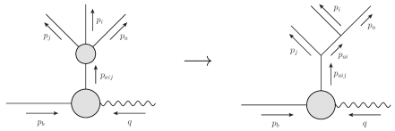
Figure 4: Kinematics mapping for final-state splittings with initial-state spectator.

Final-state splittings with initial-state spectator are treated in the same manner as final-state splittings with final-state spectator, with the sole exception of the construction of the new spectator momentum in the first branching step, if the spectator is massive. The evolution and splitting variables are defined as

$$t=\frac{2\,p_{j}p_{ai}\,p_{ai}p_{b}}{p_{aij}p_{b}}\;,\quad z_{a}=\frac{p_{a}p_{b}}{p_{aij}p_{b}}\;\qquad\text{and}\qquad s_{ai}\;,\quad x_{a}=\frac{p_{a}p_{b}}{p_{ai}p_{b}}\;$$ (75)

The new spectator momentum is defined as

$$\begin{split}p_{b}^{\,\mu}=&\;\left(\tilde{p}_{b}^{\,\mu}-\frac{q\cdot\tilde{p}_{b}}{q_{\parallel}^{2}}\,q_{\parallel}^{\,\mu}\right)\,\sqrt{\frac{\lambda(q^{2},s_{aij},m_{b}^{2})-4\,m_{b}^{2}\,\tilde{p}_{aij\perp}^{2}}{\lambda(q^{2},m_{aij}^{2},m_{b}^{2})-4\,m_{b}^{2}\,\tilde{p}_{aij\perp}^{2}}}+\frac{q^{2}+m_{b}^{2}-s_{aij}}{2\,q_{\parallel}^{2}}\,q_{\parallel}^{\,\mu}\;,\end{split}$$ (76)

where $q=\tilde{p}_{b}-\tilde{p}_{aij}$, $q_{\parallel}=q+\tilde{p}_{aij\perp}$ and $s_{aij}=(x-1)/x\,(q^{2}-m_{a}^{2})+(s_{ai}+m_{j}^{2})/x$, where

$$x=\left[\,1-\frac{t\,x_{a}/z_{a}}{q^{2}-s_{ai}-m_{j}^{2}-m_{b}^{2}}\right]^{-1}\;,\qquad\tilde{z}=\frac{z_{a}}{x_{a}}\;.$$ (77)

The remaining construction proceeds as in Sec. A.1, except that $m_{k}\to m_{b}$ and $p_{k}\to-p_{b}$. This is sketched in Fig. 4. The customary variables $y$ and $\tilde{z}$ in the second branching step are given by

$$y^{\prime}=\left[\,1+\frac{t-z_{a}/x_{a}(q^{2}-s_{ai}-m_{j}^{2}-m_{b}^{2})}{s_{ai}-m_{a}^{2}-m_{i}^{2}}\right]^{-1}\;,\quad\tilde{z}^{\prime}=x_{a}\;.$$ (78)

The phase-space factorization for final-state splittings with initial-state spectator can be derived similarly to the $2\to 3$ case described in Dittmaier (2000), App. B. We perform an s-channel factorization over $p_{aij}$ and subsequently over $p_{ai}$. This gives

$$\begin{split}\int{\rm d}\Phi(p_{a},p_{i},p_{j},K|\,p_{b},p_{c})=&\int\frac{{\rm d}s_{aij}}{2\pi}\,\int{\rm d}\Phi(p_{aij},K|\,p_{b},p_{c})\,\int{\rm d}\Phi(p_{a},p_{i},p_{j}|\,p_{aij})\\ =&\int{\rm d}\bar{x}\int{\rm d}\Phi(\tilde{p}_{aij},K|\,\tilde{p}_{b},p_{c})\,\int\Big{[}{\rm d}\Phi(p_{a},p_{i},p_{j}|\,p_{b},p_{c},q)\Big{]}\end{split}$$ (79)

where $\bar{x}=(q^{2}-m_{aij}^{2}-m_{b}^{2})/(q^{2}-s_{aij}-m_{b}^{2})$ and

$$\begin{split}\int\Big{[}{\rm d}\Phi(p_{a},p_{i},p_{j}|\,p_{b},p_{c},q)\Big{]}=&\frac{\rho_{bai}}{2\pi}\,\frac{m_{aij}^{2}+m_{b}^{2}-q^{2}}{\bar{x}^{2}}\int\frac{{\rm d}s_{ai}}{2\pi}\int\frac{1}{4(2\pi)^{2}}\frac{{\rm d}s_{bai}\,{\rm d}\phi_{ai}}{\sqrt{\lambda(s_{aij},m_{b}^{2},q^{2})}}\int{\rm d}\Phi(p_{a},p_{i}|\,p_{ai})\\ =&\frac{1}{4(2\pi)^{3}}\,\frac{\rho_{bai}}{\bar{x}}\,\frac{s_{aij}+m_{b}^{2}-q^{2}}{\sqrt{\lambda(s_{aij},m_{b}^{2},q^{2})}}\int{\rm d}s_{bai}\int{\rm d}\phi_{ai}\,\int\Big{[}{\rm d}\Phi(p_{a},p_{i}|\,p_{ai},p_{b},q)\Big{]}\;.\end{split}$$ (80)

To simplify this expression, we have used the definition Dittmaier (2000)

$$\rho_{bai}=\sqrt{\frac{\lambda((\tilde{p}_{b}+p_{c})^{2},m_{b}^{2},m_{c}^{2})}{\lambda((p_{b}+p_{c})^{2},m_{b}^{2},m_{c}^{2})}}\;,$$ (81)

We use the relation $z_{a}=(s_{ab}-m_{a}^{2}-m_{b}^{2})/(q^{2}-s_{aij}-m_{b}^{2})$ to write

$$\begin{split}\int\Big{[}{\rm d}\Phi(p_{a},p_{i}|\,p_{ai},p_{b},q)\Big{]}=&\,\int\frac{{\rm d}s_{ai}}{2\pi}\int{\rm d}\Phi(p_{a},p_{i}|\,p_{ai})=\frac{1}{4(2\pi)^{3}}\int{\rm d}s_{ai}\int{\rm d}z_{a}\int{\rm d}\phi_{a}\,\frac{s_{aij}+m_{b}^{2}-q^{2}}{\sqrt{\lambda(s_{ai},s_{bai},m_{b}^{2})}}\;.\end{split}$$ (82)

Using the auxiliary variable $\xi_{a}=z_{a}/x_{a}=(s_{bai}-s_{ai}-m_{b}^{2})/(q^{2}-s_{aij}-m_{b}^{2})$, the final result can be written as

$$\begin{split}\int\Big{[}{\rm d}\Phi(p_{a},p_{i},p_{j}|\,p_{b},p_{c},q)\Big{]}=&\,\frac{J^{(1)}_{\rm FI}}{16\pi^{2}}\int{\rm d}z_{a}\int\frac{{\rm d}\phi_{j}}{2\pi}\,\bigg{[}\,\frac{1}{16\pi^{2}}\int{\rm d}s_{ai}\int\frac{{\rm d}\xi_{a}}{\xi_{a}}\int\frac{{\rm d}\phi_{i}}{2\pi}\,J^{(2)}_{\rm FI}\,\bigg{]}\,(s_{aij}+m_{b}^{2}-q^{2})\;,\end{split}$$ (83)

where we have defined the Jacobian factors

$$J^{(1)}_{\rm FI}=\frac{\rho_{bai}}{\bar{x}}\,\frac{s_{aij}+m_{b}^{2}-q^{2}}{\sqrt{\lambda(s_{aij},m_{b}^{2},q^{2})}}\qquad\text{and}\qquad J^{(2)}_{\rm FI}=\frac{s_{ai}+m_{b}^{2}-s_{bai}}{\sqrt{\lambda(s_{ai},m_{b}^{2},s_{bai})}}\;.$$ (84)

According to Eq. (75), $s_{aij}$ (and therefore $\bar{x}$ and $\rho_{bai}$) depends on both $t$ and $s_{ai}$, hence $J^{(1)}_{\rm FI}$ is not independent of the second branching for nonzero $m_{b}$. The evolution variable could be redefined as $t=s_{aij}s_{aib}/(2p_{aij}p_{b})$ to solve this problem. As we deal with massless initial-state partons only, we defer this discussion to a future publication.

The extension of Eq. (83) to $D=4-2\varepsilon$ dimensions is straightforward. We obtain an additional factor of

$$\Delta\Phi_{\rm FI}(p_{a},p_{i},p_{j}|\,\tilde{p}_{b},\tilde{p}_{c},q)=\left(\frac{\Omega(1-2\varepsilon)}{(2\pi)^{-2\varepsilon}}\right)^{2}\left(\bar{p}_{ai,j}^{2}\sin^{2}\theta_{ai,j}^{\,b}\sin^{2}\phi_{j}\right)^{-\varepsilon}\left(\bar{p}_{a,i}^{2}\sin^{2}\theta_{a,i}^{\,b}\sin^{2}\phi_{i}\right)^{-\varepsilon}\;.$$ (85)

The momenta and polar angles are defined as in Eqs. (67) and (68), and the azimuthal angle $\phi_{i}$ is parametrized as $\phi_{i}=\phi_{a,j}^{ai,b}$, using Eq. (70). As in the case of final-state emitter with final-state spectator, the splitting functions are independent of $\phi_{j}$, hence we can average over one azimuthal angle. For massless partons, the polar angles can be written in the simple form

$$\cos\theta_{a,i}^{b}=1-2\,x_{a}\;,\qquad\cos\theta_{ai,j}^{b}=\frac{s_{aij}+s_{ai}}{s_{aij}-s_{ai}}\left[\,1-2\,\xi_{a}\,\frac{s_{aij}}{s_{aij}+s_{ai}}\right]\;.$$ (86)

The magnitudes of the momenta in this case are given by Eq. (73). In the iterated collinear limit, Eq. (85) can be simplified to give Eq. (74).

A.3 Initial-state emitter with final-state spectator

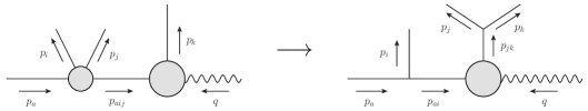
Figure 5: Kinematics mapping for initial-state splittings with final-state spectator.

The kinematics in initial-state branchings with final-state spectator is typically constructed by mapping the process to final-state branchings with initial-state spectator Catani and Seymour (1997). This mapping requires special care in the case of $2\to 4$ dipole splittings. Our algorithm is sketched in Fig. 5. We combine an initial-final branching during which the spectator is shifted off mass-shell with a $1\to 2$ decay of the newly defined pseudoparticle with momentum $p_{jk}$.

We use the following evolution and splitting variables

$$\begin{split}t=\frac{2\,p_{j}p_{ai}\,p_{ai}p_{k}}{p_{a}p_{ijk}}\;,\quad z_{a}=\frac{-q^{2}}{2\,p_{a}p_{ijk}}\qquad\text{and}\qquad s_{ai}\;,\quad x_{a}=\frac{p_{ai}p_{k}}{p_{a}p_{ijk}}\;.\end{split}$$ (87)

where $q=p_{a}-p_{i}-p_{j}-p_{k}$. We begin by constructing the initial-state branching. As the spectator parton changes its virtuality, the shift in Höche and Prestel (2015), Eq. (A.9) must be modified to

$$\begin{split}p_{jk}^{\,\mu}=&\;\left(\tilde{p}_{k}^{\,\mu}-\frac{q\cdot\tilde{p}_{k}}{q^{2}}\,q^{\,\mu}\right)\,\sqrt{\frac{\lambda(q^{2},s_{ai},s_{jk})}{\lambda(q^{2},m_{aij}^{2},m_{k}^{2})}}+\frac{q^{2}+s_{jk}-s_{ai}}{2\,q^{2}}\,q^{\,\mu}\;,\end{split}$$ (88)

where $q=\tilde{p}_{k}-\tilde{p}_{aij}$ and $s_{jk}=q^{2}(1-x_{a}/z_{a})+t/x_{a}-s_{ai}$.

Next we construct the momentum of the emitted particle, $p_{i}$, as

$$p_{i}^{\,\mu}\,= \;-\bar{z}_{i}\,\frac{\gamma(q^{2},s_{ai},s_{jk})\,p_{ai}^{\,\mu}+s_{ai}\,p_{jk}^{\,\mu}}{\beta(q^{2},s_{ai},s_{jk})}+\frac{m_{i}^{2}+{\rm k}_{\perp}^{2}}{\bar{z}_{i}}\,\frac{p_{jk}^{\,\mu}+s_{jk}/\gamma(q^{2},s_{ai},s_{jk})\,p_{ai}^{\,\mu}}{\beta(q^{2},s_{ai},s_{jk})}+k_{\perp}^{\mu}\;,$$ (89)

The parameters $\bar{z}_{i}$ and ${\rm k}_{\perp}^{2}=-k_{\perp}^{2}$ of this decomposition are given by

$$\begin{split}\bar{z}_{i}\,=&\;\frac{q^{2}-s_{ai}-s_{jk}}{\beta(q^{2},s_{ai},s_{jk})}\,\left[\;\frac{x-1}{x-u}\,-\,\frac{s_{jk}}{\gamma(q^{2},s_{ai},s_{jk})}\frac{s_{ai}+m_{i}^{2}-m_{a}^{2}}{q^{2}-s_{ai}-s_{jk}}\right]\;,\\ {\rm k}_{\perp}^{2}\,=&\;\bar{z}_{i}\,(1-\bar{z}_{i})\,s_{ai}-(1-\bar{z}_{i})\,m_{i}^{2}-\bar{z}_{i}\,m_{a}^{2}\;,\end{split}$$ (90)

where $u=-(s_{ai}-m_{i}^{2}-m_{a}^{2})\,z_{a}/q^{2}$ and $x=u+x_{a}-t\,z_{a}/(q^{2}x_{a})$.

We now boost $p_{a}$ and all final state particles into the frame where $p_{a}$ is aligned along the beam direction, with $p_{b}$, the opposite-side beam particle, unchanged. Eventually we must construct the decay of the two-parton system defined by $p_{jk}$. This can be achieved by using the same technique as in Sec. A.1, i.e. we construct a decay with the customary variables $y$ and $\tilde{z}$ defined as

$$y^{\prime}=\left[1-\frac{t/x_{a}-q^{2}x_{a}/z_{a}}{s_{jk}-m_{j}^{2}-m_{k}^{2}}\right]^{-1}\;,\qquad\tilde{z}^{\prime}=\frac{t/x_{a}}{t/x_{a}-q^{2}x_{a}/z_{a}}\;.$$ (91)

At the same time, we need to make the replacement $p_{k}\to-p_{ai}$, $m_{k}\to s_{ai}$ and use the appropriate final-state masses. This technique is sketched in Fig. 4.

The phase-space factorization for initial-state splittings with final-state spectator can be derived similarly to the $2\to 3$ case described in Dittmaier (2000), App. B. We first perform the s-channel factorization over $p_{ijk}$. Using $z_{a}=-q^{2}/(s_{ijk}+m_{a}^{2}-q^{2})$, this gives

$$\begin{split}\int{\rm d}\Phi(p_{i},p_{j},p_{k},K|\,p_{a},p_{b})=&\int\frac{{\rm d}s_{ijk}}{2\pi}\,\int{\rm d}\Phi(p_{ijk},K|\,p_{a},p_{b})\,\int{\rm d}\Phi(p_{i},p_{j},p_{k}|\,p_{ijk})\\ =&\int{\rm d}z_{a}\,\int{\rm d}\Phi(\tilde{p}_{k},K|\,\tilde{p}_{a},p_{b})\,\int\Big{[}{\rm d}\Phi(p_{i},p_{j},p_{k}|\,p_{a},p_{b},q)\Big{]}\end{split}$$ (92)

where

$$\begin{split}\int\Big{[}{\rm d}\Phi(p_{i},p_{j},p_{k}|\,p_{a},p_{b},q)\Big{]}=&\frac{1}{2\pi}\,\frac{\rho_{ija}\,q^{2}}{z_{a}^{2}}\int\frac{{\rm d}s_{jk}}{2\pi}\int\frac{1}{4(2\pi)^{2}}\frac{{\rm d}s_{ai}\,{\rm d}\phi_{i}}{\sqrt{\lambda(s_{ijk},m_{a}^{2},q^{2})}}\int{\rm d}\Phi(p_{j},p_{k}|p_{jk})\\ =&\frac{1}{4(2\pi)^{3}}\,\frac{\rho_{ija}}{z_{a}}\,\frac{s_{ijk}-m_{a}^{2}-q^{2}}{\sqrt{\lambda(s_{ijk},m_{a}^{2},q^{2})}}\int{\rm d}s_{ai}\int{\rm d}\phi_{i}\,\int\Big{[}{\rm d}\Phi(p_{j},p_{k}|p_{jk},p_{a},q)\Big{]}\;.\end{split}$$ (93)

To simplify this expression, we have used the definition Dittmaier (2000)

$$\rho_{ija}=\sqrt{\frac{\lambda((\tilde{p}_{aij}+p_{b})^{2},m_{a}^{2},m_{b}^{2})}{\lambda((p_{a}+p_{b})^{2},m_{a}^{2},m_{b}^{2})}}\;,$$ (94)

where $p_{a}^{\mu}$ is given by momentum conservation using Eq. (88). We make use of the relations $x_{a}=z_{a}\,(q^{2}-s_{aij}-s_{jk}+m_{j}^{2})/q^{2}$ and $t=-x_{a}\,(s_{aij}-s_{ai}-m_{j}^{2})$ to write

$$\begin{split}\int\Big{[}{\rm d}\Phi(p_{j},p_{k}|p_{jk},p_{a},q)\Big{]}=&\,\int\frac{{\rm d}s_{jk}}{2\pi}\int{\rm d}\Phi(p_{j},p_{k}|p_{jk})=\frac{1}{4(2\pi)^{3}}\int\frac{{\rm d}x_{a}}{x_{a}}\int{\rm d}t\int{\rm d}\phi_{j}\,\frac{-q^{2}/z_{a}}{\sqrt{\lambda(s_{jk},s_{ai},q^{2})}}\;.\end{split}$$ (95)

The final result is

$$\begin{split}\int\Big{[}{\rm d}\Phi(p_{i},p_{j},p_{k}|\,p_{a},p_{b},q)\Big{]}=&\,\frac{J^{(1)}_{\rm IF}}{16\pi^{2}}\int\frac{{\rm d}t}{t}\int\frac{{\rm d}\phi_{j}}{2\pi}\,\bigg{[}\,\frac{1}{16\pi^{2}}\int{\rm d}s_{ai}\int\frac{{\rm d}x_{a}}{x_{a}}\int\frac{{\rm d}\phi_{i}}{2\pi}\,J^{(2)}_{\rm IF}\,\bigg{]}\,\frac{t}{x_{a}}\;,\end{split}$$ (96)

where we have defined the Jacobian factors

$$J^{(1)}_{\rm IF}=\frac{\rho_{ija}}{z_{a}}\,\frac{s_{ijk}+m_{a}^{2}-q^{2}}{\sqrt{\lambda(s_{ijk},m_{a}^{2},q^{2})}}\qquad\text{and}\qquad J^{(2)}_{\rm IF}=\frac{-q^{2}\,x_{a}/z_{a}}{\sqrt{\lambda(s_{jk},s_{ai},q^{2})}}\;.$$ (97)

Note that $s_{ijk}=q^{2}(1-1/z_{a})-m_{a}^{2}$, therefore both $\rho_{ija}$ and $J^{(1)}_{\rm IF}$ are unaffected by the intrinsic branching.

The extension of Eq. (96) to $D=4-2\varepsilon$ dimensions is straightforward. We obtain an additional factor of

$$\Delta\Phi_{\rm IF}(p_{i},p_{j},p_{k}|\,\tilde{p}_{a},\tilde{p}_{b},q)=\left(\frac{\Omega(1-2\varepsilon)}{(2\pi)^{-2\varepsilon}}\right)^{2}\left(\bar{p}_{j,k}^{2}\sin^{2}\theta_{j,k}^{\,ai}\sin^{2}\phi_{j}\right)^{-\varepsilon}\left(\bar{p}_{i,jk}^{2}\sin^{2}\theta_{i,jk}^{\,a}\sin^{2}\phi_{i}\right)^{-\varepsilon}\;.$$ (98)

The momenta and polar angles are defined as in Eqs. (67) and (68), and the azimuthal angle $\phi_{i}$ is parametrized as $\phi_{i}=\phi_{a,j}^{ai,jk}$, using Eq. (70). As in the case of final-state emitter with final-state spectator, the splitting functions are independent of $\phi_{j}$, hence we can average over one azimuthal angle. For massless partons, the polar angles can be written in the simple form

$$\cos\theta_{i,jk}^{\,a}=1-\frac{2\,z_{a}(1-z_{a})s_{ai}}{q^{2}(1-x_{a})+tz_{a}/x_{a}-z_{a}s_{ai}}\;,\qquad\cos\theta_{j,k}^{\,ai}=\frac{1-2\,z_{a}t/(z_{a}t-q^{2}x_{a}^{2})}{\sqrt{1-4\,s_{ai}s_{jk}/(q^{2}x_{a}/z_{a}-t/x_{a})^{2}}}\;.$$ (99)

The magnitudes of the momenta in this case are given by

$$4\bar{p}_{i,jk}^{2}=\frac{-q^{2}}{z_{a}(1-z_{a})}\left[\,1-x_{a}+\frac{t/x_{a}-s_{ai}}{q^{2}/z_{a}}\right]^{2}\;,\qquad 4\bar{p}_{j,k}^{2}=q^{2}\left(1-\frac{x_{a}}{z_{a}}\right)+\frac{t}{x_{a}}-s_{ai}\;.$$ (100)

In the iterated double collinear limit, we thus obtain the expected result

$$\Delta\Phi_{I}(s_{aij},s_{ai},z_{a},x_{a},\phi_{i})=\frac{2\,(2\pi)^{2\varepsilon}}{\Gamma(1-2\varepsilon)}\Big{(}s_{aij}s_{ai}(1-x_{a})(1-\xi_{a})\sin^{2}\phi_{a,j}^{ai,jk}\Big{)}^{-\varepsilon}\;.$$ (101)

This result is used in Sec. III, Eq. (49) to derive the logarithmic contributions related to the phase-space integral. It shows that our choice of variables correctly identifies $z_{a}$ and $x_{a}$ with light-cone momentum fractions in the collinear limit.

A.4 Initial-state emitter with initial-state spectator

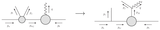
Figure 6: Kinematics mapping for initial-state splittings with initial-state spectator.

Similar to the case of initial-state splitters with final-state spectator, the kinematics in initial-state branchings with initial-state spectator requires special care in the case of $2\to 4$ dipole splittings. Our algorithm is sketched in Fig. 6. We combine an initial-initial branching during which the final-state virtuality is promoted to $(p_{j}+q)^{2}$ with a $1\to 2$ decay of the newly defined pseudoparticle into $p_{j}$ and $q$.

Our evolution and splitting variables are defined as

$$\begin{split}t=\frac{2\,p_{j}p_{ai}\,p_{ai}p_{b}}{p_{a}p_{b}}\;,\quad z_{a}=\frac{q^{2}}{2\,p_{a}p_{b}}\qquad\text{and}\qquad s_{ai}\;,\quad x_{a}=\frac{p_{ai}p_{b}}{p_{a}p_{b}}\;.\end{split}$$ (102)

We first determine the new momentum of the initial-state parton as

$$\begin{split}p_{a}^{\,\mu}=&\;\left(\tilde{p}_{aij}^{\,\mu}-\frac{\tilde{m}_{aij}^{2}}{\gamma(q^{2},\tilde{m}_{aij}^{2},m_{b}^{2})}\,p_{b}^{\,\mu}\right)\,\sqrt{\frac{\lambda(s_{ab},m_{a}^{2},m_{b}^{2})}{\lambda(q^{2},\tilde{m}_{aij}^{2},m_{b}^{2})}}+\frac{m_{a}^{2}}{\gamma(s_{ab},m_{a}^{2},m_{b}^{2})}\,p_{b}^{\,\mu}\;,\end{split}$$ (103)

where $q=p_{a}+p_{b}-p_{i}-p_{j}$ and $s_{ab}=q^{2}/z_{a}+m_{a}^{2}+m_{b}^{2}$. Next we construct the momentum of the emitted parton, $p_{j}$, as

$$p_{i}^{\,\mu}\,= \;(1-\bar{z}_{ai})\,\frac{\gamma(s_{ab},m_{a}^{2},m_{b}^{2})\,p_{a}^{\,\mu}-m_{a}^{2}\,p_{b}^{\,\mu}}{\beta(s_{ab},m_{a}^{2},m_{b}^{2})}+\frac{m_{i}^{2}+{\rm k}_{\perp}^{2}}{1-\bar{z}_{ai}}\,\frac{p_{b}^{\,\mu}-m_{b}^{2}/\gamma(s_{ab},m_{a}^{2},m_{b}^{2})\,p_{a}^{\,\mu}}{\beta(s_{ab},m_{a}^{2},m_{b}^{2})}-k_{\perp}^{\mu}\;,$$ (104)

The parameters $\bar{z}_{aij}$ and ${\rm k}_{\perp}^{2}=-k_{\perp}^{2}$ of this decomposition are given by

$$\begin{split}\bar{z}_{ai}\,=&\;\frac{s_{ab}-m_{a}^{2}-m_{b}^{2}}{\beta(s_{ab},m_{a}^{2},m_{b}^{2})}\,\left[\;x_{a}\,-\,\frac{m_{b}^{2}}{\gamma(s_{ab},m_{a}^{2},m_{b}^{2})}\frac{s_{ai}+m_{a}^{2}-m_{i}^{2}}{s_{ab}-m_{a}^{2}-m_{b}^{2}}\right]\;,\\ {\rm k}_{\perp}^{2}\,=&\;\bar{z}_{ai}\,(1-\bar{z}_{ai})\,m_{a}^{2}-(1-\bar{z}_{ai})\,s_{ai}-\bar{z}_{ai}\,m_{i}^{2}\;,\end{split}$$ (105)

In a second step, we branch the new final state momentum $p_{ai}+p_{b}$ into $p_{j}$ and $q$, using the spectator $p_{ai}$ and satisfying the constraint $q^{2}=\tilde{q}^{2}$, where $\tilde{q}=\tilde{p}_{aij}+p_{b}$. We employ the kinematics mapping of Sec. A.1. The customary variables $y$ and $\tilde{z}$ in this case are defined as

$$y^{\prime}=\left[1+\frac{q^{2}\,x_{a}/z_{a}+2s_{ai}}{q^{2}(x_{a}/z_{a}-1)+s_{ai}+m_{b}^{2}-m_{j}^{2}}\right]^{-1}\;,\qquad\tilde{z}^{\prime}=\frac{t/x_{a}}{q^{2}\,x_{a}/z_{a}+2s_{ai}}\;.$$ (106)

At the same time, we make the replacement $p_{k}\to p_{ai}$, $m_{k}\to s_{ai}$ and use the appropriate final-state masses. Finally we boost all remaining final-state particles into the frame defined by $q$, using the algorithm defined in Sec. (5.5) of Catani and Seymour (1997). The Lorentz transformation, $\Lambda$, is computed as

$$\Lambda(\tilde{q},q)^{\mu}_{\;\nu}=g^{\mu}_{\;\nu}-\frac{2\,(q+\tilde{q})^{\mu}(q+\tilde{q})_{\nu}}{(q+\tilde{q})^{2}}+\frac{2\,q^{\mu}\tilde{q}_{\nu}}{\tilde{q}^{2}}\;,$$ (107)

The phase-space factorization for initial-state splittings with initial-state spectator can be derived similar to the $2\to 3$ case described in Dittmaier (2000), App. B. We first perform the s-channel factorization over $p_{ijk}$. Using $z_{a}=q^{2}/(s_{ijq}-m_{a}^{2}-m_{b}^{2})$, this gives

$$\begin{split}\int{\rm d}\Phi(p_{i},p_{j},q|\,p_{a},p_{b})=&\int\frac{{\rm d}s_{ijq}}{2\pi}\,\int{\rm d}\Phi(p_{ijq}|\,p_{a},p_{b})\,\int{\rm d}\Phi(p_{i},p_{j},q|\,p_{ijq})\\ =&\int{\rm d}z_{a}\,\int{\rm d}\Phi(\tilde{q}|\,\tilde{p}_{a},p_{b})\,\int\Big{[}{\rm d}\Phi(p_{i},p_{j},q|\,p_{a},p_{b})\Big{]}\end{split}$$ (108)

where

$$\begin{split}\int\Big{[}{\rm d}\Phi(p_{i},p_{j},q|\,p_{a},p_{b})\Big{]}=&\frac{1}{2\pi}\frac{q^{2}}{z_{a}}\,\int\frac{{\rm d}s_{jq}}{2\pi}\int\frac{1}{4(2\pi)^{2}}\frac{{\rm d}s_{ai}\,{\rm d}\phi_{i}}{\sqrt{\lambda(s_{ab},m_{a}^{2},m_{b}^{2})}}\int{\rm d}\Phi(p_{j},q|p_{jq})\\ =&\frac{1}{4(2\pi)^{3}}\frac{q^{2}/z_{a}}{\sqrt{\lambda(s_{ab},m_{a}^{2},m_{b}^{2})}}\int{\rm d}s_{ai}\int{\rm d}\phi_{i}\,\int\Big{[}{\rm d}\Phi(p_{j},q|p_{jq},p_{a},p_{b})\Big{]}\;.\end{split}$$ (109)

We make use of the relations $x_{a}=z_{a}\,(s_{jq}-s_{ai}-m_{b}^{2})/q^{2}$ and $t=-x_{a}\,(s_{aij}-s_{ai}-m_{j}^{2})$ to write

$$\begin{split}\int\Big{[}{\rm d}\Phi(p_{j},q|p_{jq},p_{a},p_{b})\Big{]}=&\,\int\frac{{\rm d}s_{jq}}{2\pi}\int{\rm d}\Phi(p_{j},q|p_{jq})=\frac{1}{4(2\pi)^{3}}\int\frac{{\rm d}x_{a}}{x_{a}}\int{\rm d}t\int{\rm d}\phi_{j}\,\frac{q^{2}/z_{a}}{\sqrt{\lambda(s_{jq},s_{ai},m_{b}^{2})}}\;.\end{split}$$ (110)

The final result is

$$\begin{split}\int\Big{[}{\rm d}\Phi(p_{i},p_{j},q|\,p_{a},p_{b})\Big{]}=&\,\frac{J^{(1)}_{\rm II}}{4(2\pi)^{3}}\int\frac{{\rm d}t}{t}\int{\rm d}\phi_{j}\,\bigg{[}\,\frac{1}{4(2\pi)^{3}}\int{\rm d}s_{ai}\int\frac{{\rm d}x_{a}}{x_{a}}\int{\rm d}\phi_{i}\,J^{(2)}_{\rm II}\,\bigg{]}\,\frac{t}{x_{a}}\;,\end{split}$$ (111)

where we have defined the Jacobian factors

$$J^{(1)}_{\rm II}=\frac{s_{ab}-m_{a}^{2}-m_{b}^{2}}{\sqrt{\lambda(s_{ab},m_{a}^{2},m_{b}^{2})}}\qquad\text{and}\qquad J^{(2)}_{\rm II}=\frac{s_{jq}-s_{ai}-m_{b}^{2}}{\sqrt{\lambda(s_{jq},s_{ai},m_{b}^{2})}}\;,$$ (112)

and where $s_{jq}=q^{2}x_{a}/z_{a}+s_{ai}+m_{b}^{2}$.

The extension of Eq. (111) to $D=4-2\varepsilon$ dimensions is straightforward. We obtain an additional factor of

$$\Delta\Phi_{\rm II}(p_{i},p_{j},q|\,\tilde{p}_{a},\tilde{p}_{b})=\left(\frac{\Omega(1-2\varepsilon)}{(2\pi)^{-2\varepsilon}}\right)^{2}\left(\bar{p}_{j,q}^{2}\sin^{2}\theta_{j,q}^{\,ai}\sin^{2}\phi_{j}\right)^{-\varepsilon}\left(\bar{p}_{i,jq}^{2}\sin^{2}\theta_{i,jq}^{\,a}\sin^{2}\phi_{i}\right)^{-\varepsilon}\;.$$ (113)

The momenta and polar angles are defined as in Eqs. (67) and (68), and the azimuthal angle $\phi_{i}$ is parametrized as $\phi_{i}=\phi_{a,j}^{ai,jq}$, using Eq. (70). As in the case of final-state emitter with final-state spectator, the splitting functions are independent of $\phi_{j}$, hence we can average over one azimuthal angle. For massless partons, the polar angles can be written in the simple form

$$\cos\theta_{i,jq}^{\,a}=1+\frac{2\,s_{ai}}{(1-x_{a})\,q^{2}/z_{a}-s_{ai}}\;,\qquad\cos\theta_{j,q}^{\,ai}=\frac{s_{jq}+s_{ai}}{s_{jq}-s_{ai}}\left(1-2\,\frac{s_{jq}}{s_{jq}-q^{2}}\,\frac{t/x_{a}}{q^{2}x_{a}/z_{a}+2s_{ai}}\right)\,.$$ (114)

The magnitudes of the momenta in this case are given by

$$4\bar{p}_{i,jq}^{2}=\frac{q^{2}}{z_{a}}\left[\,1-x_{a}-z_{a}\frac{s_{ai}}{q^{2}}\right]^{2}\;,\qquad 4\bar{p}_{j,q}^{2}=\left(q^{2}\frac{x_{a}}{z_{a}}+s_{ai}\right)\left[1-\frac{1}{x_{a}/z_{a}+s_{ai}/q^{2}}\right]^{2}\,.$$ (115)

In the iterated collinear limit, Eq. (113) can be simplified to give Eq. (101).

References

- Gribov and Lipatov (1972) V. N. Gribov and L. N. Lipatov, Sov. J. Nucl. Phys. 15, 438 (1972).
- Lipatov (1975) L. N. Lipatov, Sov. J. Nucl. Phys. 20, 94 (1975).
- Dokshitzer (1977) Y. L. Dokshitzer, Sov. Phys. JETP 46, 641 (1977).
- Altarelli and Parisi (1977) G. Altarelli and G. Parisi, Nucl. Phys. B126, 298 (1977).
- Buckley et al. (2011) A. Buckley et al., Phys. Rept. 504, 145 (2011), arXiv:1101.2599 [hep-ph] .
- (6) J. R. Andersen et al., arXiv:1605.04692 [hep-ph] .
- Marchesini and Webber (1988) G. Marchesini and B. R. Webber, Nucl. Phys. B310, 461 (1988).
- Catani et al. (1991) S. Catani, B. R. Webber, and G. Marchesini, Nucl. Phys. B349, 635 (1991).
- Kato and Munehisa (1987) K. Kato and T. Munehisa, Phys. Rev. D36, 61 (1987).
- Kato and Munehisa (1989) K. Kato and T. Munehisa, Phys. Rev. D39, 156 (1989).
- Kato and Munehisa (1991) K. Kato and T. Munehisa, Comput. Phys. Commun. 64, 67 (1991).
- Kato et al. (1992) K. Kato, T. Munehisa, and H. Tanaka, Z. Phys. C54, 397 (1992).
- Hartgring et al. (2013) L. Hartgring, E. Laenen, and P. Skands, JHEP 10, 127 (2013), arXiv:1303.4974 [hep-ph] .
- Li and Skands (2016) H. T. Li and P. Skands, (2016), arXiv:1611.00013 [hep-ph] .
- Jadach et al. (2011) S. Jadach, A. Kusina, M. Skrzypek, and M. Slawinska, JHEP 08, 012 (2011), arXiv:1102.5083 [hep-ph] .
- Gituliar et al. (2014) O. Gituliar, S. Jadach, A. Kusina, and M. Skrzypek, Phys. Lett. B732, 218 (2014), arXiv:1401.5087 [hep-ph] .
- Jadach et al. (2016) S. Jadach, A. Kusina, W. Placzek, and M. Skrzypek, JHEP 08, 092 (2016), arXiv:1606.01238 [hep-ph] .
- Plätzer and Sjödahl (2012) S. Plätzer and M. Sjödahl, (2012), arXiv:1206.0180 [hep-ph] .
- Nagy and Soper (2015) Z. Nagy and D. E. Soper, JHEP 07, 119 (2015), arXiv:1501.00778 [hep-ph] .
- Nagy and Soper (2016) Z. Nagy and D. E. Soper, JHEP 10, 019 (2016), arXiv:1605.05845 [hep-ph] .
- Curci et al. (1980) G. Curci, W. Furmanski, and R. Petronzio, Nucl. Phys. B175, 27 (1980).
- Furmanski and Petronzio (1980) W. Furmanski and R. Petronzio, Phys. Lett. B97, 437 (1980).
- Floratos et al. (1981a) E. G. Floratos, R. Lacaze, and C. Kounnas, Phys. Lett. B98, 89 (1981a).
- Floratos et al. (1981b) E. G. Floratos, R. Lacaze, and C. Kounnas, Phys. Lett. B98, 285 (1981b).
- Catani and Grazzini (2000) S. Catani and M. Grazzini, Nucl. Phys. B570, 287 (2000), hep-ph/9908523 [hep-ph] .
- Höche et al. (2010) S. Höche, S. Schumann, and F. Siegert, Phys. Rev. D81, 034026 (2010), arXiv:0912.3501 [hep-ph] .
- Lönnblad (2012) L. Lönnblad, (2012), arXiv:1211.7204 [hep-ph] .
- Catani and Seymour (1997) S. Catani and M. H. Seymour, Nucl. Phys. B485, 291 (1997), hep-ph/9605323 .
- Jadach and Skrzypek (2004) S. Jadach and M. Skrzypek, Acta Phys. Polon. B35, 745 (2004), hep-ph/0312355 .
- Procura and Stewart (2010) M. Procura and I. W. Stewart, Phys. Rev. D81, 074009 (2010), [Erratum: Phys. Rev.D83,039902(2011)], arXiv:0911.4980 [hep-ph] .
- Jain et al. (2011) A. Jain, M. Procura, and W. J. Waalewijn, JHEP 05, 035 (2011), arXiv:1101.4953 [hep-ph] .
- Heinrich and Kunszt (1998) G. Heinrich and Z. Kunszt, Nucl. Phys. B519, 405 (1998), hep-ph/9708334 .
- (33) R. K. Ellis and W. Vogelsang, hep-ph/9602356 .
- Ritzmann and Waalewijn (2014) M. Ritzmann and W. J. Waalewijn, Phys. Rev. D90, 054029 (2014), arXiv:1407.3272 [hep-ph] .
- Gehrmann-De Ridder et al. (2004) A. Gehrmann-De Ridder, T. Gehrmann, and G. Heinrich, Nucl. Phys. B682, 265 (2004), hep-ph/0311276 .
- Dokshitzer et al. (2006) Y. L. Dokshitzer, G. Marchesini, and G. P. Salam, Phys. Lett. B634, 504 (2006), arXiv:hep-ph/0511302 .
- Frixione and Webber (2002) S. Frixione and B. R. Webber, JHEP 06, 029 (2002), hep-ph/0204244 .
- Somogyi et al. (2005) G. Somogyi, Z. Trocsanyi, and V. Del Duca, JHEP 06, 024 (2005), hep-ph/0502226 .
- Höche and Prestel (2015) S. Höche and S. Prestel, Eur. Phys. J. C75, 461 (2015), arXiv:1506.05057 [hep-ph] .
- Sjöstrand (1985) T. Sjöstrand, Phys. Lett. B157, 321 (1985).
- Sjöstrand et al. (2015) T. Sjöstrand, S. Ask, J. R. Christiansen, R. Corke, N. Desai, P. Ilten, S. Mrenna, S. Prestel, C. O. Rasmussen, and P. Z. Skands, Comput. Phys. Commun. 191, 159 (2015), arXiv:1410.3012 [hep-ph] .
- Gleisberg et al. (2004) T. Gleisberg, S. Höche, F. Krauss, A. Schälicke, S. Schumann, and J. Winter, JHEP 02, 056 (2004), hep-ph/0311263 .
- Gleisberg et al. (2009) T. Gleisberg, S. Höche, F. Krauss, M. Schönherr, S. Schumann, F. Siegert, and J. Winter, JHEP 02, 007 (2009), arXiv:0811.4622 [hep-ph] .
- Lai et al. (2010) H.-L. Lai, M. Guzzi, J. Huston, Z. Li, P. M. Nadolsky, et al., Phys.Rev. D82, 074024 (2010), arXiv:1007.2241 [hep-ph] .
- Catani et al. (2002) S. Catani, S. Dittmaier, M. H. Seymour, and Z. Trocsanyi, Nucl. Phys. B627, 189 (2002), hep-ph/0201036 .
- Dittmaier (2000) S. Dittmaier, Nucl. Phys. B565, 69 (2000), hep-ph/9904440 .