An Almost Analytical Approach to Simulating 2D Electronic Spectra

Abstract

We introduce an almost analytical method to simulate 2D electronic spectra as a double Fourier transform of the the non-linear response function (NRF) corresponding to a particular optical pulse sequence. We employ a unitary transformation to represent the total system Hamiltonian in a stationary basis that allows us to separate contributions from decoherence and phonon-mediated population relaxation to the NRF. Previously, one of us demonstrated the use of an analytic, cumulant expansion approach to calculate the decoherence term. Here, we extend this idea to obtain an accurate expression for the population relaxation term, a significant improvement over standard quantum master equation-based approximations. We numerically demonstrate the accuracy of our method by computing the photon echo spectrum of a two-level system coupled to a thermal bath, and we highlight the mechanistic insights obtained from our simulation.

1 Introduction

2D Electronic Spectroscopy is a four wave mixing technique ^{1, 2, 3, 4, 5, 6, 7, 8, 9, 10, 11, 12} that can, uniquely, report on excitonic transitions, couplings and relaxation pathways. These measurements provide invaluable insights into the mechanisms of energy transport in biological processes including, most notably, photosynthetic light harvesting complexes. However, theoretical simulations are essential to correctly interpret measured 2D electronic spectra by disentangling the contributions from different mechanistic pathways ^{13, 14, 15, 16, 17}.

Existing theoretical approaches can be broadly classified into two categories. The first includes methods developed to calculate net nonlinear polarization using either nonperturbative approaches ^{15, 18, 19} or time-nonlocal quantum master equation based approaches ^{16, 20}. However, nonperturbative methods provide limited molecular insights and in general, the calculated nonlinear polarization must be subjected to significant post-processing to extract the signal due to a particular pulse sequence ²¹. The second category of methods directly calculate nonlinear response functions (NRFs) that correspond to a particular pulse sequence. Existing approaches include analytic perturbative methods based on early work ^{22, 23}, however they rely on adhoc approximations including an artificial separation of decoherence and population relaxation contributions to the NRF making them inaccurate descriptors of dynamics particularly at short times ¹³. Liouville space heirarchical equations of motion have also been used to calculate NRFs numerically ¹⁷, however, these methods are computationally expensive and scale poorly with system dimensionality.

In this paper, we introduce a novel, near analytic, computationally efficient method for the theoretical calculation of NRFs. We focus on the simulation of a 2D Photon Echo spectrum ^{24, 25, 26, 14} but our approach is general and can be trivially extended to other types of measurements. Our method is derived through a series of well defined approximations and has several key features: a) First, we use a unitary transformation, introduced previously, ^{27, 28} to map adiabatic states to a stationary basis, that allows us to rigorously decouple decoherence from the exciton relaxation dynamics, b) Second, we treat dynamics during the coherence and rephasing times ($t_{1}$ and $t_{3}$, respectively), and the population time $(t_{2})$ with the same level of approximation making our approach accurate at both short and long times, c) Third, the decoherence contribution to the NRF is evaluated analytically for systems where the bath is well described by either an Ohmic or a Debye spectral distribution. The population relaxation term is evaluated through a series of simple numerical integrations. d) Finally, we treat doubly excited states populated in the Excited State Absorption (ESA) pathway ¹³ on an even footing with singly excited states with no additional approximations. Taken together, these features render this approach very powerful and the near analytic formulation makes it computationally inexpensive and easy to implement. By properly separating contributions to the spectrum from decoherence and population relaxation pathways, we are able to provide necessary mechanistic insights.

The paper is organized as follows. First, in Section 2, we introduce the stationary basis and the unitary mapping transformation employed to represent the total Hamiltonian for an $n$-level system coupled to a thermal bath in this framework. Next, in Section 3, we briefly review NRF and the computation of 2D photon echo electronic spectrum. We then introduce our approach for the Stimulated Emission (SE) pathway in Section 4 outlining the calculation of both the decoherence contribution and our new approach to evaluate the population relaxation contribution. In Section 5, we provide similar outlines for both the Ground State Bleaching (GSB) and Excited State Absorption (ESA) pathways both of which contribute to the 2D photon echo spectrum. We then demonstrate the results of our simulation for a model two-level system and discuss the key insights obtained in Section 6.

2 Stationary Basis

The quantum mechanical Hamiltonian for an $n$-level system where each state is linearly coupled to a thermal bath of harmonic oscillators can be written as

$$\bar{H}=\epsilon_{g}|g\rangle\langle g|+H_{\text{ad}}(\textbf{Q})+H_{\text{ph}},$$ (1)

where

$$H_{\text{ad}}(\textbf{Q}) = \sum_{j}\epsilon_{j}|j\rangle\langle j|+\sum_{i,j;i\neq j}J_{ij}|i\rangle\langle j|$$ (2)

$$+ \sum_{j}Q_{j}|j\rangle\langle j|,$$

and

$$H_{ph}=\sum_{j,b}\frac{1}{2}\left(\frac{p_{jb}^{2}}{m_{jb}}+m_{jb}\omega_{jb}^{2}q_{jb}^{2}\right).$$ (3)

In Eq. 2, $i$ and $j$ label the local first excited states, $\epsilon_{j}$ is the energy of the $j^{th}$ state, $J_{ij}$ is the electronic coupling between the $i^{th}$ and $j^{th}$ states, and $\epsilon_{g}$ is the ground state energy of the full system. Further, in Eq. 2 and Eq. 3, $Q_{j}=\sum_{b}m_{jb}\nu_{jb}q_{jb}$, where $m_{jb}$, $q_{jb}$, $p_{jb}$, and $\omega_{jb}$ are, respectively, the mass, position, momentum, and angular frequency associated with the $b^{th}$ harmonic bath mode coupled to the $j^{th}$ state of the system.

We now define a set of adiabatic eigenfunctions ^{27, 28} such that

$$H_{ad}(\textbf{Q})|m(\textbf{Q})\rangle=\varepsilon_{m}(\textbf{Q})|m(\textbf{Q})\rangle,$$ (4)

where we introduce the notation $\mathbf{Q}=\{Q_{j}\}$. We recognize that the $\mathbf{Q}$-dependent adiabatic eigenfunctions do not commute with momentum operators in $H_{ph}$. Therefore, we introduce a new stationary basis, $|m(\textbf{Q}=\textbf{0})\rangle$, that is $\mathbf{Q}$-independent and that we will denote simply as $|m\rangle$ in the remainder of this manuscript. We then define a unitary transformation from the adiabatic basis to our stationary basis ^{27, 28},

$$|m(\textbf{Q})\rangle=U(\textbf{Q})|m\rangle.$$ (5)

Defining $H=U^{{\dagger}}(\textbf{Q})\bar{H}U(\textbf{Q})$, the unitary transformation of the Hamiltonian in Eq. 1, and introducing two physically reasonable approximations, we obtain

$$H=H_{0}+H_{\text{na}},$$ (6)

where

$$H_{0}=\epsilon_{g}|g\rangle\langle g|+\sum_{m}\varepsilon_{m}(\textbf{Q})|m\rangle\langle m|+H_{\text{ph}}$$ (7)

is a diagonal matrix in the stationary state basis and $H_{\text{ph}}$ is defined previously in Eq. 3. The part of the Hamiltonian that drives nonadiabatic transitions in Eq. 6 is defined as

$$H_{\text{na}}=\frac{1}{2}\sum_{j}(P_{j}A^{j}(\textbf{0})+A^{j}(\textbf{0})P_{j}),$$ (8)

where $P_{j}=\sum_{b}\nu_{jb}p_{jb}$ and the matrix elements of the nonadiabatic coupling vector are defined as

$$A^{j}_{n,m}(\textbf{0})=-i\frac{\langle n(\textbf{0})|j\rangle\langle j|m(\textbf{0})\rangle}{\varepsilon_{n}(\textbf{0})-\varepsilon_{m}(\textbf{0})}.$$ (9)

The two approximations mentioned above are both used to derive the nonadiabatic Hamiltonian in Eq. 8. Applying an exact unitary transformation to the Hamiltonian in Eq. 1, we obtain a nonadiabatic coupling vector where the $j^{\text{th}}$ component is defined as

$$A^{j}(\textbf{Q})=\sum_{n,m}A^{j}_{n,m}(\textbf{Q})|n\rangle\langle m|,$$ (10)

with matrix elements,

$$A^{j}_{n,m}(\textbf{Q}) = -i\langle n(\textbf{Q})|\frac{\partial}{\partial Q_{j}}m(\textbf{Q})\rangle$$ (11)

$$= -i\frac{\langle n(\textbf{Q})|j\rangle\langle j|m(\textbf{Q})\rangle}{\varepsilon_{n}(\textbf{Q})-\varepsilon_{m}(\textbf{Q})},$$

where we use the Hellmann-Feynman theorem to obtain the second equality. Since both the numerator, involving overlaps between stationary states and local excited states, and the denominator, the energy gap term, are likely to be robust with respect to phonon-induced fluctuations, we first approximate the nonadiabatic coupling vector by its value at $\mathbf{Q}=\textbf{0}$, i.e. $A^{j}(\mathbf{Q})\approx A^{j}(\textbf{0})$. Second, treating the nonadiabatic coupling term perturbatively, we assume that terms which are second order in $A^{j}(\mathbf{Q})$ are negligible.

3 Simulating the Photon Echo Spectrum

Stimulated photon echo electronic spectroscopy is a three pulse UV-vis experiment, with phase matching direction $\textbf{k}_{S}=-\textbf{k}_{1}+\textbf{k}_{2}+\textbf{k}_{3}$. Here, we provide a concise definition for the 2D Photon Echo spectrum in terms of the relevant response functions. A more detailed description is available in the literature ^{13, 25, 16}.

We calculate the 2D photon echo spectrum from the expression ²⁵

$$\tilde{S}_{\text{PE}}(\omega_{1},t_{2},\omega_{3}) =\int_{0}^{\infty}dt_{3}e^{i\omega_{3}t_{3}}\int_{-\infty}^{\infty}dt_{1}e^{-i\omega_{1}t_{1}}$$

$$\times S_{\text{PE}}(t_{3},t_{2},t_{1}),$$ (12)

where $\omega_{1}$ and $\omega_{3}$ are fourier transform frequencies. The time-domain photon echo signal in Eq. 12 is defined in terms of response functions,

$$S_{PE}(t_{3},t_{2},t_{1}) =K[R_{\text{SE}}(t_{3},t_{2},t_{1})$$

$$+R_{\text{GSB}}(t_{3},t_{2},t_{1})-R^{*}_{\text{ESA}}(t_{3},t_{2},t_{1})],$$ (13)

where $K$ is a common prefactor containing the dot products of the transition dipole moment unit vectors with the electric fields ¹. The three response functions in Eq. 13 correspond to three different pathways – (i) Stimulated Emission (SE), $R_{\text{SE}}$ (ii) Ground State Bleaching (GSB), $R_{\text{GSB}}$, and (iii) Excited State Absorption (ESA), $R^{*}_{\text{ESA}}$. The polarization contribution from each pathway has sign $(-1)^{n}$, where $n$ is the number of bra-side field-matter interactions. In this case, the contribution from the ESA pathway is negative whereas the other two are positive.

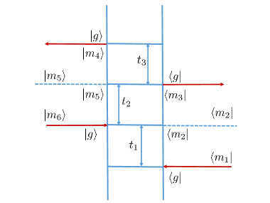
4 The SE Pathway

We introduce our formulation in the context of the SE pathway, diagrammatically represented in Fig. 1. The response function corresponding to this pathway can be written as ¹³

$$R_{\text{SE}}(t_{3},t_{2},t_{1}) =\langle\mu(0)\mu(t_{1}+t_{2})\mu(t_{1}+t_{2}+t_{3})$$

$$\times\mu(t_{1})\rho(0)\rangle,$$ (14)

where $\rho(0)=|g\rangle\langle g|\rho_{ph}(0)$. Writing the time evolved transition dipole moment operator as ${\mu(t)=e^{i\bar{H}t}\mu e^{-i\bar{H}t}}$, we obtain,

$$R_{\text{SE}}(t_{3},t_{2},t_{1}) =Tr_{ph}\big{\{}\langle g|\mu e^{i\bar{H}t_{1}}e^{i\bar{H}t_{2}}\mu e^{i\bar{H}t_{3}}\mu$$

$$\times e^{-i\bar{H}t_{3}}e^{-i\bar{H}t_{2}}\mu e^{-i\bar{H}t_{1}}|g\rangle\rho_{\text{ph}}(0)\big{\}}.$$ (15)

Introducing a complete set of adiabatic states and then unitary transforming to the stationary basis, $|m\rangle$, as defined in Eq. 5, we obtain

$$R_{\text{SE}} (t_{3},t_{2},t_{1})=\sum_{\{m\}}Tr_{ph}\big{\{}\langle g|\mu|m_{1}\rangle\langle m_{1}|e^{iHt_{1}}|m_{2}\rangle$$

$$\times\langle m_{2}|e^{iHt_{2}}|m_{3}\rangle\langle m_{3}|\mu|g\rangle\langle g|e^{iHt_{3}}|g\rangle\langle g|\mu|m_{4}\rangle$$

$$\times\langle m_{4}|e^{-iHt_{3}}|m_{5}\rangle\langle m_{5}|e^{-iHt_{2}}|m_{6}\rangle\langle m_{6}|\mu|g\rangle$$

$$\times\langle g|e^{-iHt_{1}}|g\rangle\rho_{\text{ph}}(0)\big{\}},$$ (16)

where we use the index $\{m\}$ in the summation to denote a full sum over the set of states $\{m_{1},\ m_{2},\ m_{3},\ m_{4},\ m_{5},\ m_{6}\}$. Furthermore, in Eq. 16, since the transition dipole matrix element between the ground and an adiabatic excited electronic state can be reasonably assumed to be independent of Q, we make the approximation, $\langle g|\mu|m_{1}(\textbf{Q})\rangle\approx\langle g|\mu|m_{1}\rangle$. Extracting the transition dipole matrix elements from the phonon trace in Eq. 16, we can write

$$R_{\text{SE}}(t_{3},t_{2},t_{1})=\sum_{\{m\}}\mu_{gm_{1}}\mu_{m_{3}g}\mu_{gm_{4}}\mu_{m_{6}g}$$

$$\times e^{i\epsilon_{g}(t_{3}-t_{1})}Tr_{ph}\big{\{}\langle m_{1}|e^{iHt_{1}}|m_{2}\rangle\langle m_{2}|e^{iHt_{2}}|m_{3}\rangle$$

$$\times\langle m_{4}|e^{-iHt_{3}}|m_{5}\rangle\langle m_{5}|e^{-iHt_{2}}|m_{6}\rangle e^{iH_{\text{ph}}t_{3}}$$

$$\times e^{-iH_{\text{ph}}t_{1}}\rho_{\text{ph}}(0)\big{\}},$$ (17)

and we have used $\langle g|e^{iHt}|g\rangle=e^{i\epsilon_{g}t}e^{iH_{\text{ph}}t}$.

Figure 1: Stimulated Emission (SE) pathway where the system-field interactions are shown with red arrows.

To evaluate individual matrix elements in Eq. 17, we introduce a complete set of states in the stationary adiabatic basis and the identity operator, $\hat{1}=e^{-iH_{0}t}e^{iH_{0}t}$, to obtain

$$\langle m_{1}|e^{iHt_{1}}|m_{2}\rangle =\langle m_{1}|e^{iHt_{1}}e^{-iH_{0}t_{1}}|m_{2}\rangle$$

$$\times\langle m_{2}|e^{iH_{0}t_{1}}|m_{2}\rangle.$$ (18)

Using the definition of the time evolution operator in the interaction picture,

$$U_{I}(t)=e^{iH_{0}t}e^{-iHt},$$ (19)

and evaluating time evolution under the zeroth order Hamiltonian we obtain,

$$e^{-iH_{0}t}|m\rangle=\left(\hat{T}e^{-i\int^{t}_{0}dt^{\prime}\varepsilon(\textbf{Q}(t^{\prime}))}\right)e^{-iH_{\text{ph}}t}|m\rangle,$$ (20)

where $\textbf{Q}(t^{\prime})=e^{iH_{\text{ph}}t^{\prime}}\textbf{Q}e^{-iH_{\text{ph}}t^{\prime}}$ and $\hat{T}$ is the time-ordering operator ²⁷. This allows us to write Eq. 18 as

$$\langle m_{1}|e^{iHt_{1}}|m_{2}\rangle =\langle m_{1}|U_{I}^{{\dagger}}(t_{1})|m_{2}\rangle$$

$$\times\left(\hat{T}^{{\dagger}}e^{i\int^{t_{1}}_{0}dt^{\prime}\varepsilon_{m_{2}}(\textbf{Q}(t^{\prime}))}\right)e^{iH_{ph}t_{1}}.$$ (21)

Further, recognizing that the matrix elements of the time-evolution operator in the interaction picture are ²⁹

$$\langle m|U_{I}(t)|n\rangle=(\hat{T}e^{-i\int^{t}_{0}dt^{\prime}H_{na}(t^{\prime})})_{m,n},$$ (22)

allows us to re-write the expression in Eq. 21 as

$$\langle m_{1}|e^{iHt_{1}}|m_{2}\rangle =\left(\hat{T}^{{\dagger}}e^{i\int^{t1}_{0}dt^{\prime}H_{na}(t^{\prime})}\right)_{m_{1},m_{2}}$$

$$\times\left(\hat{T}^{{\dagger}}e^{i\int^{t_{1}}_{0}dt^{\prime}\varepsilon_{m_{2}}(\textbf{Q}(t^{\prime}))}\right)e^{iH_{ph}t_{1}},$$ (23)

where $H_{na}$ is previously defined in Eq. 8, and $H_{na}(t)~{}=~{}e^{iH_{0}(t)}H_{na}e^{-iH_{0}(t)}$.

The terms in Eq. 23 yield significant physical insight. Terms in the exponent that contain $H_{na}$ depend on momenta and give rise to nonadiabatic transitions that cause population relaxation. The remaining terms in the exponent depend on bath position coordinates, $\varepsilon_{m}(\textbf{Q}(t^{\prime}))$), and account for environment driven fluctuations in the energies of the stationary states and cause decoherence.

Taylor expanding $\varepsilon_{m}(\textbf{Q})$ about $\textbf{Q}=0$ to first order, we obtain

$$\hat{T}e^{-i\int^{t}_{0}dt^{\prime}\varepsilon_{m}(\textbf{Q}(t^{\prime}))} =e^{-i\varepsilon_{m}t}$$

$$\times\left(\hat{T}e^{-i\int^{t}_{0}dt^{\prime}\nabla_{\textbf{Q}}\varepsilon_{m}(\textbf{Q}(t^{\prime}))\cdot\textbf{Q}(t^{\prime})}\right),$$ (24)

where $\nabla_{\textbf{Q}}\varepsilon_{m}(\textbf{Q}(t^{\prime}))$ is the gradient. Substituting Eq. 23 and Eq. 24 into the product of matrix elements in Eq. 17, we obtain

$$R_{\text{SE}} (t_{3},t_{2},t_{1})=\sum_{\{m\}}\mu_{gm_{1}}\mu_{m_{3}g}\mu_{gm_{4}}\mu_{m_{6}g}$$

$$\times e^{i(\varepsilon_{m_{2}}-\epsilon_{g})t_{1}}e^{i(\varepsilon_{m_{3}}-\varepsilon_{m_{5}})t_{2}}e^{-i(\varepsilon_{m_{4}}-\epsilon_{g})t_{3}}$$

$$\times F_{\text{SE}}(t_{1},t_{2},t_{3}),$$ (25)

where the pre-exponential factor is defined as

$$F_{\text{SE}}(t_{1},t_{2},t_{3})=\big{\langle}\left(1-D_{\text{SE}}(t_{1},t_{2},t_{3})\right)$$

$$\times\left(\delta_{m_{1},m_{2}}\delta_{m_{2},m_{3}}\delta_{m_{4},m_{5}}\delta_{m_{5},m_{6}}-P_{\text{SE}}(t_{1},t_{2},t_{3})\right)\big{\rangle},$$ (26)

and we use $\langle\cdot\rangle$ as short-hand for the phonon trace $\text{Tr}\{\ldots\rho_{ph}(0)\}$. In Eq. 26, the decoherence term is defined as

$$D_{\text{SE}}(t_{1}, t_{2},t_{3})=1-\left((\hat{T}^{{\dagger}}e^{i\int^{t_{1}}_{0}dt^{\prime}\nabla_{\textbf{Q}}\varepsilon_{m_{2}}(\textbf{Q}(t^{\prime}))\cdot\textbf{Q}(t^{\prime})})\right.$$

$$\times(\hat{T}^{{\dagger}}e^{i\int^{t_{2}}_{0}dt^{\prime}\nabla_{\textbf{Q}}\varepsilon_{m_{3}}(\textbf{Q}(t^{\prime}))\cdot\textbf{Q}(t^{\prime})})$$

$$\times(\hat{T}e^{-i\int^{t_{3}}_{0}dt^{\prime}\nabla_{\textbf{Q}}\varepsilon_{m_{4}}(\textbf{Q}(t^{\prime}))\cdot\textbf{Q}(t^{\prime})})$$

$$\left.\times(\hat{T}e^{-i\int^{t_{2}}_{0}dt^{\prime}\nabla_{\textbf{Q}}\varepsilon_{m_{5}}(\textbf{Q}(t^{\prime}))\cdot\textbf{Q}(t^{\prime})})\right),$$ (27)

and the population relaxation term is defined as

$$P_{\text{SE}}(t_{1},t_{2},t_{3}) =\delta_{m_{1},m_{2}}\delta_{m_{2},m_{3}}\delta_{m_{4},m_{5}}\delta_{m_{5},m_{6}}$$

$$-\left(\left(\hat{T}^{{\dagger}}e^{i\int^{t_{1}}_{0}dt^{\prime}H_{na}(t^{\prime})}\right)_{m_{1},m_{2}}\right.$$

$$\times\left(\hat{T}^{{\dagger}}e^{i\int^{t_{2}}_{0}dt^{\prime}H_{na}(t^{\prime})}\right)_{m_{2},m_{3}}$$

$$\times\left(\hat{T}e^{-i\int^{t_{3}}_{0}dt^{\prime}H_{na}(t^{\prime})}\right)_{m_{4},m_{5}}$$

$$\left.\times\left(\hat{T}e^{-i\int^{t_{2}}_{0}dt^{\prime}H_{na}(t^{\prime})}\right)_{m_{5},m_{6}}\right).$$ (28)

It is worth noting that the expressions for $D_{\text{SE}}(t_{1},t_{2},t_{3})$ and $P_{\text{SE}}(t_{1},t_{2},t_{3})$ are dependent on the values of $m_{1}$, $m_{2}$, $m_{3}$, $m_{4}$, $m_{5}$ and $m_{6}$, respectively but the dependence is not explicitly stated in $D_{\text{SE}}(t_{1},t_{2},t_{3})$ and $P_{\text{SE}}(t_{1},t_{2},t_{3})$ to avoid cluttering.

4.1 Cumulant Expansion

The decoherence and population relaxation terms in Eq. 27 and Eq. 28 respectively are evaluated using a second order cumulant expansion ¹. While one of us has previously used this approach to evaluate the decoherence term ^{27, 28}, here we propose a cumulant expansion approach to treat the population relaxation term as well, eliminating the need for master equation based methods. A significant benefit of this approach is its computational efficiency: the decoherence term can be evaluated analytically for Ohmic and Debye spectral density functions and the population relaxation term can be calculated using simple numerical integration.

We consider two cases in evaluating Eq. 26:
Case 1: $\delta_{m_{1},m_{2}}\delta_{m_{2},m_{3}}\delta_{m_{4},m_{5}}\delta_{m_{5},m_{6}}=1$, where the conditions $m_{1}=m_{2}=m_{3}$ and $m_{4}=m_{5}=m_{6}$ are both satisfied. Neglecting the coupling between the decoherence and population relaxation term and using a second order cumulant expansion we obtain,

$$F_{\text{SE}}( t_{1},t_{2},t_{3})$$

$$\approx 1-\big{\langle}D_{\text{SE}}(t_{1},t_{2},t_{3})\big{\rangle}-\big{\langle}P_{\text{SE}}(t_{1},t_{2},t_{3})\big{\rangle}$$

$$\approx e^{-\big{(}\big{\langle}\bar{D}_{\text{SE}}(t_{1},t_{2},t_{3})\big{\rangle}+\big{\langle}\bar{P}_{\text{SE}}(t_{1},t_{2},t_{3})\big{\rangle}\big{)}},$$ (29)

where $\bar{D}_{\text{SE}}(t_{1},t_{2},t_{3})$ and $\bar{P}_{\text{SE}}(t_{1},t_{2},t_{3}))$ involve a series of single and double time integrals detailed in the appendix A and B respectively. We note that $\bar{D}_{\text{SE}}$ is analytically determined for thermal baths described by Ohmic or Debye spectral densities and can be numerically evaluated for a general spectral density function.
Case 2: $\delta_{m_{1},m_{2}}\delta_{m_{2},m_{3}}\delta_{m_{4},m_{5}}\delta_{m_{5},m_{6}}=0$. As in the previous case, neglecting the coupling between decoherence and population relaxation

$$F_{\text{SE}}(t_{1},t_{2},t_{3})\approx\big{\langle}-P_{\text{SE}}\big{\rangle}=\big{\langle}1-\left(1+P_{\text{SE}}\right)\big{\rangle}.$$ (30)

Using a second order cumulant expansion, we obtain

$$F_{\text{SE}}(t_{1},t_{2},t_{3})\approx 1-e^{\big{\langle}\bar{P}_{\text{SE}}(t_{1},t_{2},t_{3})\big{\rangle}},$$ (31)

where $\bar{P}_{\text{SE}}$ is defined in the Appendix B.

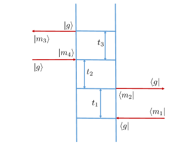
5 GSB and ESA Pathways

Figure 2: The GSB pathway where system field interactions are indicated by red arrows

The response function for the Ground State Bleaching (GSB) pathway shown in Fig. 2 is ¹³

$$R_{\text{GSB}}(t_{3},t_{2},t_{1}) =\langle\mu(0)\mu(t_{1})\mu(t_{1}+t_{2}+t_{3})$$

$$\times\mu(t_{1}+t_{2})\rho_{0}\rangle.$$ (32)

Extracting the transition dipole matrix elements and introducing complete sets of stationary states, we obtain

$$R_{\text{GSB}}(t_{3},t_{2},t_{1})=\sum_{\{m\}}\mu_{gm_{1}}\mu_{m_{2}g}\mu_{gm_{3}}\mu_{m_{4}g}$$

$$\times Tr_{ph}\big{\{}\rho_{ph}(0)\langle m_{1}|e^{i\bar{H}t_{1}}|m_{2}\rangle\langle g|e^{i\bar{H}(t_{2}+t_{3})}|g\rangle$$

$$\times\langle m_{3}|e^{-i\bar{H}t_{3}}|m_{4}\rangle\langle g|e^{-i\bar{H}(t_{1}+t_{2})}|g\rangle\big{\}}.$$ (33)

Evaluating the matrix elements in Eq. 33, and using a second order cumulant expansion to approximate the decoherence and population relaxation terms, we arrive at an easily evaluated expression for the response function. The final expression along with the derivation details are provided in Appendix C.

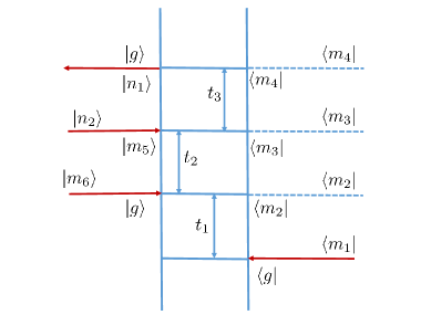
Figure 3: The ESA pathway where system field interactions are indicated by red arrows

The Excited State Absorption (ESA) pathway involves both the singly and doubly excited states. Local doubly excited state are represented as $|i,j\rangle$, with the condition $i<j$ to avoid double counting of states. The electronic coupling between a pair of doubly excited states is given as $\langle i,j|\bar{H}|i_{1},j_{2}\rangle=J_{i,j_{2}}$ if $j=i_{1}$ and $\langle i,j|\bar{H}|i_{1},j_{2}\rangle=J_{j,j_{2}}$ if $i=i_{1}$ and zero otherwise. The response function for the ESA pathway shown in Fig. 3 is then given as ¹³

$$R^{*}_{\text{ESA}}(t_{3},t_{2},t_{1}) =\langle\mu(0)\mu(t_{1}+t_{2}+t_{3})$$

$$\times\mu(t_{1}+t_{2})\mu(t_{1})\rho_{0}\rangle.$$ (34)

As before, we extract the transition dipole matrix elements from the trace and introduce the $|m\rangle$ stationary states obtained by unitary transforming singly excited adiabatic states and $|n\rangle$ stationary states obtained by unitary transforming doubly excited adiabatic states.

$$R^{*}_{\text{ESA}}(t_{3},t_{2},t_{1})=\sum_{\{m,n\}}\mu_{gm_{1}}\mu_{m_{4}n_{1}}\mu_{n_{2}m_{5}}\mu_{m_{6}g}$$

$$\times Tr_{ph}\big{\{}\rho_{ph}(0)\langle m_{1}|e^{i\bar{H}t_{1}}|m_{2}\rangle\langle m_{2}|e^{i\bar{H}t_{2}}|m_{3}\rangle$$

$$\times\langle m_{3}|e^{i\bar{H}t_{3}}|m_{4}\rangle\langle n_{1}|e^{-i\bar{H}t_{3}}|n_{2}\rangle\langle m_{5}|e^{-i\bar{H}t_{2}}|m_{6}\rangle$$

$$\times\langle g|e^{-i\bar{H}t_{1}}|g\rangle\big{\}}.$$ (35)

We note that transitions from the singly excited states, $|m_{i}\rangle$, to the doubly excited states, $|n_{i}\rangle$, are only induced by the applied electric field and not via phonon-mediated population relaxation. The final expression for the ESA response function and derivation details for the same are provided in Appendix D.

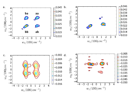
6 Results and Discussion

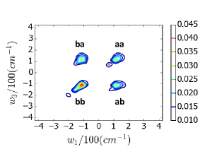
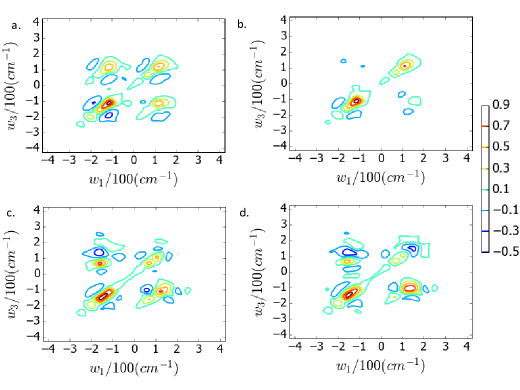
Figure 4: Contribution to the response function from the SE and ESA pathways at different $t_{2}$: (a) SE contribution at $t_{2}=10\ fs$, (b) SE contribution at $t_{2}=625\ fs$, (c) ESA contribution at $t_{2}=10\ fs$, and (d) ESA contribution at $t_{2}=625\ fs$.

Figure 5: Contribution to the response function from the GSB pathway at $t_{2}=10\ fs$.

We calculate the 2D electronic spectrum for a two-level system where the Hamiltonian $\bar{H}$ (see Eq. 1) is given as,

$$\bar{H} =\epsilon_{g}|g\rangle\langle g|+\epsilon_{1}|1\rangle\langle 1|+\epsilon_{2}|2\rangle\langle 2|+J_{12}|1\rangle\langle 2|$$

$$+J_{21}|2\rangle\langle 1|+Q_{1}|1\rangle\langle 1|+Q_{2}|2\rangle\langle 2|+H_{ph},$$

where $\epsilon_{g}=-12000\ cm^{-1}$, $\epsilon_{1}=-50\ cm^{-1}$, $\epsilon_{2}=50\ cm^{-1}$ and $J_{12}=J_{21}=100\ cm^{-1}$. Transforming to the stationary basis (see Eq. 7), we have states $a$ and $b$ with energies $\varepsilon_{a}(\textbf{Q}=\mathbf{0})=111.803\ cm^{-1}$ and $\varepsilon_{b}(\textbf{Q}=\mathbf{0})=-111.803\ cm^{-1}$. The thermal bath (environment) is modeled by an Ohmic spectral density, given as

$$S(\omega)=\frac{\lambda}{\omega_{c}}\omega e^{-\omega/\omega_{c}},$$ (37)

where $\lambda$ is the reorganization energy and $\omega_{c}$ is the phonon relaxation frequency. We use the values $\frac{\lambda}{\omega_{c}}=1.2$, $\omega_{c}=53\ cm^{-1}$, and temperature $T=77\ K$. We further assume that the transition dipole $\mu_{ga}=\mu_{gb}$.

The three pathways contribute different spectral features to the overall 2D spectrum at different times. The diagonal peaks in the spectrum are labeled, $\bf{aa}$ centered at $\omega_{1}=\omega_{3}=\omega_{a}$ and $\bf{bb}$ centered at $\omega_{1}=\omega_{3}=\omega_{b}$, and the off-diagonal peaks are labeled, $\bf{ab}$ centered at $\omega_{1}=\omega_{a}\;,\omega_{3}=\omega_{b}$ and $\bf{ba}$ centered at $\omega_{1}=\omega_{b}\;,\omega_{3}=\omega_{a}$.

For the SE pathway, at $t_{2}=0$, the populations are centered at the diagonal peaks $\bf{aa}$ and $\bf{bb}$, respectively and the coherences are centered at the off-diagonal peaks $\bf{ab}$ and $\bf{ba}$, respectively. Fig. 4(a) shows the contributions from the populations (peaks $\bf{aa}$ and $\bf{bb}$) and coherences (peaks $\bf{ab}$ and $\bf{ba}$) at a short time $t_{2}=10\ fs$. It is to be noted that at short times, phonon-mediated population transfer is insignificant as phonons are not thermally activated yet. However, at longer times, the thermally activated phonons result in a population transfer from $a$ to $b$, resulting in an emerging off-diagonal peak at $\bf{ab}$ and decreasing intensity at $\bf{aa}$. Similarly, we will have population relaxation from $b$ to $a$, leading to an off-diagonal peak at $\bf{ba}$ and decreasing intensity at $\bf{bb}$. Again, the rate of downhill relaxation ($a\rightarrow b$) is greater than that of the uphill relaxation pathway ($b\rightarrow a$), resulting in a larger intensity at $\bf{ab}$ compared to $\bf{ba}$. Decoherence, on the other hand, leads to decreasing contributions from coherences at the peaks $\bf{ab}$ and $\bf{ba}$ with increasing $t_{2}$. Fig. 4(b) shows the SE pathway contributions from both populations and coherences at $t_{2}=625\ fs$. Decoherence is effectively complete and population relaxation, as discussed above, leads to large intensities at the peaks $\bf{bb}$ and $\bf{ab}$, respectively and a decrease in intensity at $\bf{aa}$. At $77\ K$, thermal energy is insufficient to access the uphill pathway $b\rightarrow a$, hence there is effectively no peak due to population relaxation at $\bf{ba}$.

The ESA pathway, at $t_{2}=0$, results in off-diagonal peaks, $\bf{ab}$ and $\bf{ba}$ for populations at $a$ and at $b$, respectively and coherences at peaks $\bf{bb}$ and $\bf{aa}$, respectively. As discussed before, the intensity contributions from the ESA pathway are negative. Fig. 4(c) shows the populations at off-diagonal peaks and coherences at diagonal peaks at $t_{2}=10\ fs$. At longer times, decoherence will result in decreasing contributions from coherences and downhill population relaxation ($a\rightarrow b$) will result in a decreased contribution at $\bf{ab}$ and a rise in negative intensity at $\bf{aa}$. The negative intensity at $\bf{ba}$, on the other hand, does not change much since uphill population relaxation is insignificant at $T=77\ K$. These features are seen in Fig. 4(d), which shows the ESA pathway contributions at $t_{2}=625\ fs$.

In the GSB pathway, there is only ground state dynamics during $t_{2}$. Hence, the excited state populations at the diagonal peaks and coherences at the off-diagonal peaks do not evolve with $t_{2}$ (see Fig. 5).

Figure 6: 2D photon echo electronic spectra at different $t_{2}$: (a) $10\ fs$, (b) $100\ fs$, (c) $300\ fs$ and (d) $625\ fs$.

The overall spectrum arising from the contributions of the SE, GSB and ESA pathways are shown for different times in Figs. 6(a)-(d). Immediate and marked differences could be spotted at short and long $t_{2}$, respectively. At short $t_{2}$ (see Fig. 6(a), $t_{2}=10\ fs$), we have positive intensities arising mostly from populations at the peaks $\bf{aa}$ and $\bf{bb}$ and coherences at the off-diagonal peaks $\bf{ab}$ and $\bf{ba}$. Fig. 6(b) shows the spectrum at $t_{2}=100\ fs$. Decoherence is complete and a small peak is seen emerging at $\bf{ab}$, due to the downhill population relaxation $a\rightarrow b$ in SE pathway. Fig. 6(c) shows the spectrum at $t_{2}=300\ fs$. The crosspeak at $\bf{ab}$ has increased in intensity, with a concomitant decrease in intensity at $\bf{aa}$. A negative intensity is also seen at $\bf{ba}$, arising from the ESA pathway due to population at $b$. Fig. 6(d) shows the spectrum at $t_{2}=625\ fs$. The intensities at $\bf{bb}$ and $\bf{ab}$ (due to population relaxation from $a$ to $b$) are large and positive, whereas negative intensities, arising from the ESA pathway are seen at peaks $\bf{ba}$ (large negative intensity due to population at $b$) and $\bf{aa}$ (due to $a\rightarrow b$ relaxation). Also, decoherence is complete.

7 Conclusions

We introduce a new method for simulating electronic 2DPES (2D Photon Echo Spectroscopy). We transform to a stationary basis and employ the cumulant expansion approach to evaluate decoherence and population relaxation. We demonstrate the efficiency of our new approach for a model two level system. We capture all the features expected from 2DPES, the most prominent of them being an emerging off-diagonal peak (at $\bf{ab}$) at long $t_{2}$ from the SE pathway due to population relaxation from the higher to the lower energy exciton, as well as a negative off-diagonal peak (at $\bf{ba}$) arising from the ESA pathway. The coherences decay with time and have oscillatory behavior, in contrast to exciton population relaxation, which is reflected by a steady decrease/increase in the relevant peaks. We will leverage the computational efficiency of our approach to simulate energy transfer in higher dimensional systems.

8 Acknowledgements

The authors acknowledge the Cornell startup funding and DOE NMGC seed funding. The authors are also grateful to Professor K. L. Sebastian for helpful discussions.

Appendices

Appendix A: Decoherence in the Stimulated Emission Pathway

$\bar{D}_{\text{SE}}(t_{1},t_{2},t_{3})$, when written out in full, contains several second order time-ordered terms. These involve integration with respect to two different time arguments, $t$ and $s$, over an integrand, which, when traced over, has the general form,

$$d_{m,n}(t,s) =\big{\langle}(\nabla_{\textbf{Q}}\varepsilon_{m}(\textbf{Q}(t))\cdot\textbf{Q}(t))$$

$$\times(\nabla_{\textbf{Q}}\varepsilon_{n}(\textbf{Q}(s))\cdot\textbf{Q}(s))\big{\rangle}.$$ (S1)

We neglect the minimal contribution from the higher order derivatives $\frac{\partial^{n}\varepsilon_{m}}{\partial Q_{j}^{n}}$, where $n>1$ and $j$ labels the site/chromophore ²⁸. For an uncorrelated bath, this gives

$$d_{m,n}(t,s)=\sum_{j}\big{(}\frac{\partial\varepsilon_{m}}{\partial Q_{j}}\big{)}\big{(}\frac{\partial\varepsilon_{n}}{\partial Q_{j}}\big{)}\big{\langle}Q_{j}(t)Q_{j}(s)\big{\rangle}.$$ (S2)

Noting that $Q_{j}=\sum_{b}m_{jb}\nu_{jb}q_{jb}$, Eq. S2 can be written as

$$d_{m,n}(t,s) =\int^{\infty}_{0}d\omega S(\omega)\big{(}\coth(\frac{\beta\omega}{2})$$

$$\times\cos(\omega(t-s))-i\sin(\omega(t-s))\big{)}.$$ (S3)

Here, $S(\omega)$ is the spectral density modeling the environment and is defined as $S(\omega)=\sum_{b}\frac{m_{jb}\nu_{jb}^{2}}{2\omega_{jb}}\delta(\omega-\omega_{jb})$. $\bar{D}_{\text{SE}}(t_{1},t_{2},t_{3})$ is obtained analytically for the Ohmic and Debye spectral densities. For other specific spectral densities, this needs to be obtained numerically and involves at most $10$ numerical integrations which are easily evaluated (see Eq. S8).

The SE pathway decoherence, $\bar{D}_{\text{SE}}(t_{1},t_{2},t_{3})$, contains 4 types of terms:

(a) a first order term,

$$\int^{t}_{0}dt^{\prime}(\nabla_{\textbf{Q}}\varepsilon_{m}(\textbf{Q}(t^{\prime}))\cdot\textbf{Q}(t^{\prime})),$$ (S4)

which when traced over, gives zero as ${\big{\langle}Q_{j}(t)\big{\rangle}=0}$,

(b) a time-ordered second order term

$$X_{m}(t)=\int^{t}_{0}dt^{\prime}\int^{t^{\prime}}_{0}dt^{\prime\prime}(\nabla_{\textbf{Q}}\varepsilon_{m}(\textbf{Q}(t^{\prime}))\cdot\textbf{Q}(t^{\prime}))\\ (\nabla_{\textbf{Q}}\varepsilon_{m}(\textbf{Q}(t^{\prime\prime}))\cdot\textbf{Q}(t^{\prime\prime})),$$ (S5)

(c) a second order term given by a product of two first order terms with different time arguments $t$ and $s$

$$Y_{m,n}(t,s)=\int^{t}_{0}dt^{\prime}\int^{s}_{0}dt^{\prime\prime}(\nabla_{\textbf{Q}}\varepsilon_{m}(\textbf{Q}(t^{\prime}))\cdot\textbf{Q}(t^{\prime}))\\ (\nabla_{\textbf{Q}}\varepsilon_{n}(\textbf{Q}(t^{\prime\prime}))\cdot\textbf{Q}(t^{\prime\prime})),$$ (S6)

(d) a second order term given by a product of two first order terms with the same time argument $t$

$$Z_{m,n}(t)=\int^{t}_{0}dt^{\prime}\int^{t}_{0}dt^{\prime\prime}(\nabla_{\textbf{Q}}\varepsilon_{m}(\textbf{Q}(t^{\prime}))\cdot\textbf{Q}(t^{\prime}))\\ (\nabla_{\textbf{Q}}\varepsilon_{n}(\textbf{Q}(t^{\prime\prime}))\cdot\textbf{Q}(t^{\prime\prime})).$$ (S7)

The second order terms are evaluated analytically for the Ohmic spectral density (Eq. 37) ^{27, 28}.

$\bar{D}_{\text{SE}}(t_{1},t_{2},t_{3})$ is given as,

$$\bar{D}_{\text{SE}}(t_{1},t_{2},t_{3}) =X^{{\dagger}}_{m_{2}}(t_{1})+X^{{\dagger}}_{m_{3}}(t_{2})+X_{m_{4}}(t_{3})$$

$$+X_{m_{5}}(t_{2})+Y_{m_{2},m_{3}}(t_{1},t_{2})$$

$$-Y_{m_{2},m_{4}}(t_{1},t_{3})-Y_{m_{2},m_{5}}(t_{1},t_{2})$$

$$-Y_{m_{3},m_{4}}(t_{2},t_{3})-Z_{m_{3},m_{5}}(t_{2})$$

$$+Y_{m_{4},m_{5}}(t_{3},t_{2}).$$ (S8)

In Eq. 29, the quantity $\big{\langle}\bar{D}_{\text{SE}}(t_{1},t_{2},t_{3})\big{\rangle}$ is the decoherence term $\bar{D}_{\text{SE}}(t_{1},t_{2},t_{3})$ traced with respect to the bath degrees of freedom, given as

$$\big{\langle}\bar{D}_{\text{SE}}(t_{1},t_{2},t_{3})\big{\rangle} =\big{\langle}X^{{\dagger}}_{m_{2}}(t_{1})+X^{{\dagger}}_{m_{3}}(t_{2})+X_{m_{4}}(t_{3})$$

$$+X_{m_{5}}(t_{2})+Y_{m_{2},m_{3}}(t_{1},t_{2})$$

$$-Y_{m_{2},m_{4}}(t_{1},t_{3})-Y_{m_{2},m_{5}}(t_{1},t_{2})$$

$$-Y_{m_{3},m_{4}}(t_{2},t_{3})-Z_{m_{3},m_{5}}(t_{2})$$

$$+Y_{m_{4},m_{5}}(t_{3},t_{2})\big{\rangle}.$$ (S9)

Appendix B: Population Relaxation in the Stimulated Emission Pathway

$\bar{P}_{\text{SE}}(t_{1},t_{2},t_{3})$, when written out in full, contains several second order time-ordered terms. These involve integration, with respect to two different time arguments, $t$ and $s$, over an integrand, which, when traced over, has the general form

$$\big{\langle}H_{na,kl}(t)H_{na,mn}(s)\big{\rangle} \approx\sum_{j}A^{j}_{k,l}(\textbf{0})A^{j}_{m,n}(\textbf{0})$$

$$e^{i\triangle\varepsilon_{kl}t}e^{i\triangle\varepsilon_{mn}s}\big{\langle}\hat{P}_{j}(t)\hat{P}_{j}(s)\big{\rangle}.$$ (S10)

Here, $H_{na}(t)$ is defined in the interaction picture, where $H_{0}$ is given in Eq. 7, $H_{na}$ in Eq. 8 and $\triangle\varepsilon_{kl}=\varepsilon_{k}-\varepsilon_{l}$. The approximation in Eq. S10 arises because we use $e^{iH_{0}t}|m\rangle\approx e^{i\varepsilon_{m}t}|m\rangle$. $\big{\langle}P_{j}(t)P_{j}(s)\big{\rangle}$ can be easily evaluated to give

$$\big{\langle}P_{j}(t)P_{j}(s)\big{\rangle} =\int^{\infty}_{0}d\omega S(\omega)\omega^{2}$$

$$\times\bigg{(}\frac{e^{-i\omega(t-s)}}{1-e^{-\beta\omega}}+\frac{e^{i\omega(t-s)}}{e^{\beta\omega}-1}\bigg{)}.$$ (S11)

Therefore, we have

$$\big{\langle}H_{na,kl}(t)H_{na,mn}(s)\big{\rangle}\approx\sum_{j}A^{j}_{k,l}(\textbf{0})A^{j}_{m,n}(\textbf{0})$$

$$\times\int^{\infty}_{0}d\omega S(\omega)\omega^{2}\bigg{(}\frac{e^{i(\triangle\varepsilon_{kl}-\omega)t}e^{i(\triangle\varepsilon_{mn}+\omega)s}}{1-e^{-\beta\omega}}$$

$$+\frac{e^{i(\triangle\varepsilon_{kl}+\omega)t}e^{i(\triangle\varepsilon_{mn}-\omega)s}}{e^{\beta\omega}-1}\bigg{)}.$$ (S12)

The integration in Eq. S12 is easily performed numerically. The population relaxation term for the SE pathway, $\bar{P}_{\text{SE}}(t_{1},t_{2},t_{3})$, again, contains four types of terms:
(a) a first order term, $\int^{t}_{0}dt^{\prime}H_{{na},mn}(t^{\prime})$, which, when traced over, gives zero as $\langle\hat{P}_{j}(t)\rangle=0$,
(b) a time-ordered second order term

$$L_{m,n}(t)=\int^{t}_{0}dt^{\prime}\int^{t^{\prime}}_{0}dt^{\prime\prime}(H_{na}(t^{\prime})H_{na}(t^{\prime\prime}))_{mn},$$ (S13)

(c) a second order term given by a product of two first order terms with different time arguments $t$ and $s$

$$N_{k,l,m,n}(t,s) =\int^{t}_{0}dt^{\prime}\int^{s}_{0}dt^{\prime\prime}(H_{{na},kl}(t^{\prime})$$

$$\times H_{{na},mn}(t^{\prime\prime})),$$ (S14)

(d) a second order term given by a product of two first order terms with the same time argument $t$

$$O_{k,l,m,n}(t) =\int^{t}_{0}dt^{\prime}\int^{t}_{0}dt^{\prime\prime}(H_{{na},kl}(t^{\prime})$$

$$\times H_{{na},mn}(t^{\prime\prime})).$$ (S15)

The second order terms are easily evaluated numerically, using Mathematica. $\bar{P}_{\text{SE}}(t_{1},t_{2},t_{3})$ is given as,

$$\bar{P}_{\text{SE}}(t_{1},t_{2},t_{3}) =\delta_{m_{1},m_{2}}\delta_{m_{2},m_{3}}\delta_{m_{4},m_{5}}L_{m_{5},m_{6}}(t_{2})$$

$$+\delta_{m_{1},m_{2}}\delta_{m_{2},m_{3}}\delta_{m_{5},m_{6}}L_{m_{4},m_{5}}(t_{3})$$

$$+\delta_{m_{1},m_{2}}\delta_{m_{4},m_{5}}\delta_{m_{5},m_{6}}L^{{\dagger}}_{m_{2},m_{3}}(t_{2})$$

$$+\delta_{m_{2},m_{3}}\delta_{m_{4},m_{5}}\delta_{m_{5},m_{6}}L^{{\dagger}}_{m_{1},m_{2}}(t_{1})$$

$$+\delta_{m_{1},m_{2}}\delta_{m_{2},m_{3}}N_{m_{4},m_{5},m_{5},m_{6}}(t_{3},t_{2})$$

$$-\delta_{m_{1},m_{2}}\delta_{m_{4},m_{5}}O_{m_{2},m_{3},m_{5},m_{6}}(t_{2})$$

$$-\delta_{m_{2},m_{3}}\delta_{m_{4},m_{5}}N_{m_{1},m_{2},m_{5},m_{6}}(t_{1},t_{2})$$

$$-\delta_{m_{1},m_{2}}\delta_{m_{5},m_{6}}N_{m_{2},m_{3},m_{4},m_{5}}(t_{2},t_{3})$$

$$-\delta_{m_{2},m_{3}}\delta_{m_{5},m_{6}}N_{m_{1},m_{2},m_{4},m_{5}}(t_{1},t_{3})$$

$$+\delta_{m_{4},m_{5}}\delta_{m_{5},m_{6}}N_{m_{1},m_{2},m_{2},m_{3}}(t_{1},t_{2}).$$ (S16)

Solving Eq. S16 is easy but can be expensive as the number of levels increases. However, it is worth noting that we have already incorporated memory/coherence effects in the expression for decoherence and Eq. S16 contains only the incoherent population relaxation effects. Therefore, we make the approximation of neglecting the coupling of population relaxation effects during various time intervals (the $N$ terms) and use only the terms which contain population relaxation happening during one time interval (the $L$ and $O$ terms). Eq. S16, therefore, reduces to

$$\bar{P}_{\text{SE}}(t_{1},t_{2},t_{3}) \approx\delta_{m_{1},m_{2}}\delta_{m_{2},m_{3}}\delta_{m_{4},m_{5}}L_{m_{5},m_{6}}(t_{2})$$

$$+\delta_{m_{1},m_{2}}\delta_{m_{2},m_{3}}\delta_{m_{5},m_{6}}L_{m_{4},m_{5}}(t_{3})$$

$$+\delta_{m_{1},m_{2}}\delta_{m_{4},m_{5}}\delta_{m_{5},m_{6}}L^{{\dagger}}_{m_{2},m_{3}}(t_{2})$$

$$+\delta_{m_{2},m_{3}}\delta_{m_{4},m_{5}}\delta_{m_{5},m_{6}}L^{{\dagger}}_{m_{1},m_{2}}(t_{1})$$

$$-\delta_{m_{1},m_{2}}\delta_{m_{4},m_{5}}O_{m_{2},m_{3},m_{5},m_{6}}(t_{2}).$$ (S17)

In Eq. 29, the quantity $\big{\langle}\bar{P}_{\text{SE}}(t_{1},t_{2},t_{3})\big{\rangle}$ is the population relaxation term $\bar{P}_{\text{SE}}(t_{1},t_{2},t_{3})$ traced with respect to the bath degrees of freedom, given as

$$\big{\langle}\bar{P}_{\text{SE}}(t_{1},t_{2},t_{3})\big{\rangle} \approx\big{\langle}\delta_{m_{1},m_{2}}\delta_{m_{2},m_{3}}\delta_{m_{4},m_{5}}L_{m_{5},m_{6}}(t_{2})$$

$$+\delta_{m_{1},m_{2}}\delta_{m_{2},m_{3}}\delta_{m_{5},m_{6}}L_{m_{4},m_{5}}(t_{3})$$

$$+\delta_{m_{1},m_{2}}\delta_{m_{4},m_{5}}\delta_{m_{5},m_{6}}L^{{\dagger}}_{m_{2},m_{3}}(t_{2})$$

$$+\delta_{m_{2},m_{3}}\delta_{m_{4},m_{5}}\delta_{m_{5},m_{6}}L^{{\dagger}}_{m_{1},m_{2}}(t_{1})$$

$$-\delta_{m_{1},m_{2}}\delta_{m_{4},m_{5}}O_{m_{2},m_{3},m_{5},m_{6}}(t_{2})\big{\rangle}.$$ (S18)

Evaluating $\bar{P}_{\text{SE}}(t_{1},t_{2},t_{3})$, thus, requires at most $5$ numerical integrations (see Eq. S17).

Appendix C: Ground State Bleaching Response Function

We provide a brief derivation of the GSB response function here. We have, from Eq. 32,

$$R_{\text{GSB}}(t_{3},t_{2},t_{1}) =\sum_{\{m\}}\mu_{gm_{1}}\mu_{m_{2}g}\mu_{gm_{3}}\mu_{m_{4}g}$$

$$e^{i(\varepsilon_{m_{2}}-\epsilon_{g})t_{1}}e^{-i(\varepsilon_{m_{3}}-\epsilon_{g})t_{3}}$$

$$F_{\text{GSB}}(t_{1},t_{2},t_{3}),$$ (S19)

where

$$F_{\text{GSB}}(t_{1},t_{2},t_{3}) =\big{\langle}(1-D_{\text{GSB}}(t_{1},t_{2},t_{3}))$$

$$(\delta_{m_{1},m_{2}}\delta_{m_{3}m_{4}}-P_{\text{GSB}}(t_{1},t_{2},t_{3}))\big{\rangle},$$ (S20)

where

$$D_{\text{GSB}}(t_{1},t_{2},t_{3}) =1-(\hat{T}^{{\dagger}}e^{i\int^{t_{1}}_{0}dt^{\prime}\nabla_{\textbf{Q}}\varepsilon_{m_{2}}(\textbf{Q}(t^{\prime}))\cdot\textbf{Q}(t^{\prime})})$$

$$\times(\hat{T}e^{-i\int^{t_{3}}_{0}dt^{\prime}\nabla_{\textbf{Q}}\varepsilon_{m_{3}}(\textbf{Q}(t^{\prime}))\cdot\textbf{Q}(t^{\prime})}),$$ (S21)

and

$$P_{\text{GSB}}(t_{1},t_{2},t_{3}) =\delta_{m_{1},m_{2}}\delta_{m_{3}m_{4}}$$

$$-(\hat{T}^{{\dagger}}e^{i\int^{t_{1}}_{0}dt^{\prime}H_{na}(t^{\prime})})_{m_{1},m_{2}}$$

$$(\hat{T}e^{-i\int^{t_{3}}_{0}dt^{\prime}H_{na}(t^{\prime})})_{m_{3},m_{4}}.$$ (S22)

Again, there could be two cases:

1. $\delta_{m_{1},m_{2}}\delta_{m_{3},m_{4}}=1$. We neglect the coupling between decoherence and population relaxation and then use the second order cumulant expansion to obtain

$$F_{\text{GSB}}(t_{1},t_{2},t_{3}) =\big{\langle}(1-D_{\text{GSB}}(t_{1},t_{2},t_{3}))$$

$$\times(1-P_{\text{GSB}}(t_{1},t_{2},t_{3}))\big{\rangle}$$

$$\approx e^{-\big{(}\big{\langle}\bar{D}_{\text{GSB}}(t_{1},t_{2},t_{3})\big{\rangle}+\big{\langle}\bar{P}_{\text{GSB}}(t_{1},t_{2},t_{3})\big{\rangle}\big{)}}.$$ (S23)

$\bar{D}_{\text{GSB}}(t_{1},t_{2},t_{3})$ and $\bar{P}_{\text{GSB}}(t_{1},t_{2},t_{3})$ are defined below.

2. $\delta_{m_{1},m_{2}}\delta_{m_{3},m_{4}}=0$. In a way similar to the SE pathway, after decoupling decoherence and population relaxation and using the second order cumulant expansion, we have

$$F_{\text{GSB}}(t_{1},t_{2},t_{3})=\big{(}1-e^{\big{\langle}\bar{P}^{GSB}(t_{1},t_{2},t_{3})\big{\rangle}}\big{)}.$$ (S24)

Here,

$$\bar{D}_{\text{GSB}}(t_{1},t_{2},t_{3}) =X^{{\dagger}}_{m_{2}}(t_{1})+X_{m_{3}}(t_{3})$$

$$-Y_{m_{2},m_{3}}(t_{1},t_{3}),$$ (S25)

where $X_{m}(t)$ and $Y_{m,n}(t,s)$ have been defined in Eqs. S5-S6 before. Also,

$$\bar{P}_{\text{GSB}}(t_{1},t_{2},t_{3}) =\delta_{m_{1},m_{2}}L_{m_{3},m_{4}}(t_{3})$$

$$+\delta_{m_{3},m_{4}}L^{{\dagger}}_{m_{1},m_{2}}(t_{1})$$

$$-N_{m_{1},m_{2},m_{3},m_{4}}(t_{1},t_{3}),$$ (S26)

where $L_{m,n}(t)$ and $N_{k,l,m,n}(t,s)$ are defined in Eqs. S13-S14. We could neglect the coupling between population relaxations during different time intervals to obtain

$$\bar{P}_{\text{GSB}}(t_{1},t_{2},t_{3}) \approx\delta_{m_{1},m_{2}}L_{m_{3},m_{4}}(t_{3})$$

$$+\delta_{m_{3},m_{4}}L^{{\dagger}}_{m_{1},m_{2}}(t_{1}).$$ (S27)

Appendix D: Excited State Absorption Response Function

We provide a brief derivation of the ESA response function here. We have from Eq. 35,

$$R^{*}_{\text{ESA}}(t_{3},t_{2},t_{1}) =\sum_{\{m,n\}}\mu_{gm_{1}}\mu_{m_{4}n_{1}}\mu_{n_{2}m_{5}}\mu_{m_{6}g}$$

$$e^{i(\varepsilon_{m_{2}}-\epsilon_{g})t_{1}}e^{i(\varepsilon_{m_{3}}-\varepsilon_{m_{5}})t_{2}}$$

$$e^{i(\varepsilon_{m_{4}}-\varepsilon_{n_{1}})t_{3}}F_{\text{ESA}}(t_{1},t_{2},t_{3}),$$ (S28)

where

$$F_{\text{ESA}}(t_{1},t_{2},t_{3}) =\big{\langle}(1-D_{\text{ESA}}(t_{1},t_{2},t_{3}))$$

$$\times(\delta_{m_{1},m_{2}}\delta_{m_{2},m_{3}}\delta_{m_{3}m_{4}}\delta_{n_{1},n_{2}}\delta_{m_{5},m_{6}}$$

$$-P_{\text{ESA}}(t_{1},t_{2},t_{3}))\big{\rangle}.$$ (S29)

Here,

$$D_{\text{ESA}}(t_{1},t_{2},t_{3}) =1-(\hat{T}^{{\dagger}}e^{i\int^{t_{1}}_{0}dt^{\prime}\nabla_{\textbf{Q}}\varepsilon_{m_{2}}(\textbf{Q}(t^{\prime}))\cdot\textbf{Q}(t^{\prime})})$$

$$\times(\hat{T}^{{\dagger}}e^{i\int^{t_{2}}_{0}dt^{\prime}\nabla_{\textbf{Q}}\varepsilon_{m_{3}}(\textbf{Q}(t^{\prime}))\cdot\textbf{Q}(t^{\prime})})$$

$$\times(\hat{T}^{{\dagger}}e^{i\int^{t_{3}}_{0}dt^{\prime}\nabla_{\textbf{Q}}\varepsilon_{m_{4}}(\textbf{Q}(t^{\prime}))\cdot\textbf{Q}(t^{\prime})})$$

$$\times(\hat{T}e^{-i\int^{t_{3}}_{0}dt^{\prime}\nabla_{\textbf{Q}}\varepsilon_{n_{1}}(\textbf{Q}(t^{\prime}))\cdot\textbf{Q}(t^{\prime})})$$

$$\times(\hat{T}e^{-i\int^{t_{2}}_{0}dt^{\prime}\nabla_{\textbf{Q}}\varepsilon_{m_{5}}(\textbf{Q}(t^{\prime}))\cdot\textbf{Q}(t^{\prime})}),$$ (S30)

and

$$P_{\text{ESA}}(t_{1},t_{2},t_{3}) =\delta_{m_{1},m_{2}}\delta_{m_{2},m_{3}}\delta_{m_{3}m_{4}}\delta_{n_{1},n_{2}}\delta_{m_{5},m_{6}}$$

$$-(\hat{T}^{{\dagger}}e^{i\int^{t_{1}}_{0}dt^{\prime}H_{na}(t^{\prime})})_{m_{1},m_{2}}$$

$$\times(\hat{T}^{{\dagger}}e^{i\int^{t_{2}}_{0}dt^{\prime}H_{na}(t^{\prime})})_{m_{2},m_{3}}$$

$$\times(\hat{T}^{{\dagger}}e^{i\int^{t_{3}}_{0}dt^{\prime}H_{na}(t^{\prime})})_{m_{3},m_{4}}$$

$$\times(\hat{T}e^{-i\int^{t_{3}}_{0}dt^{\prime}H_{na}(t^{\prime})})_{n_{1},n_{2}}$$

$$\times(\hat{T}e^{-i\int^{t_{2}}_{0}dt^{\prime}H_{na}(t^{\prime})})_{m_{5},m_{6}}.$$ (S31)

The Kronecker-delta constraints give us two cases, as before.

1. $\delta_{m_{1},m_{2}}\delta_{m_{2},m_{3}}\delta_{m_{3}m_{4}}\delta_{n_{1},n_{2}}\delta_{m_{5},m_{6}}=1$. This gives

$$F_{\text{ESA}}(t_{1},t_{2},t_{3})) =\big{\langle}(1-D_{\text{ESA}}(t_{1},t_{2},t_{3}))$$

$$\times(1-P_{\text{ESA}}(t_{1},t_{2},t_{3}))\big{\rangle}$$

$$\approx e^{-\big{(}\big{\langle}\bar{D}_{\text{ESA}}(t_{1},t_{2},t_{3})\big{\rangle}+\big{\langle}\bar{P}_{\text{ESA}}(t_{1},t_{2},t_{3})\big{\rangle}\big{)}}.$$ (S32)

$\bar{D}_{\text{ESA}}(t_{1},t_{2},t_{3})$, $\bar{P}_{\text{ESA}}(t_{1},t_{2},t_{3})$ are defined below.

2. $\delta_{m_{1},m_{2}}\delta_{m_{2},m_{3}}\delta_{m_{3}m_{4}}\delta_{n_{1},n_{2}}\delta_{m_{5},m_{6}}=0$. Using second order cumulant expansion for decoherence and population relaxation and neglecting the coupling between decoherence and population relaxation, we have

$$F_{\text{ESA}}(t_{1},t_{2},t_{3})) \approx\big{(}1-e^{\big{\langle}\bar{P}_{\text{ESA}}(t_{1},t_{2},t_{3})\big{\rangle}}\big{)}.$$ (S33)

Here,

$$\bar{D}_{\text{ESA}}(t_{1},t_{2},t_{3})=X^{{\dagger}}_{m_{2}}(t_{1})+X^{{\dagger}}_{m_{3}}(t_{2})+$$

$$X^{{\dagger}}_{m_{4}}(t_{3})+X_{n_{1}}(t_{3})+X_{m_{5}}(t_{2})+Y_{m_{2},m_{3}}(t_{1},t_{2})$$

$$+Y_{m_{2},m_{4}}(t_{1},t_{3})-Y_{m_{2},n_{1}}(t_{1},t_{3})-Y_{m_{2},m_{5}}(t_{1},t_{2})$$

$$+Y_{m_{3},m_{4}}(t_{2},t_{3})-Y_{m_{3},n_{1}}(t_{2},t_{3})-Z_{m_{3},m_{5}}(t_{2})$$

$$-Z_{m_{4},n_{1}}(t_{3})-Y_{m_{4},m_{5}}(t_{3},t_{2})+Y_{n_{1},m_{5}}(t_{3},t_{2}),$$ (S34)

where $X_{m,n}(t)$, $Y_{m,n}(t,s)$ and $Z_{m,n}(t)$ are defined in Eqs. S5-S7. The second order population relaxation term, after neglecting the couplings during different time intervals, is given as

$$\bar{P}_{\text{ESA}}(t_{1},t_{2},t_{3}) =$$

$$\delta_{m_{2},m_{3}}\delta_{m_{3},m_{4}}\delta_{m_{5},m_{6}}\delta_{n_{1},n_{2}}L^{{\dagger}}_{m_{1},m_{2}}(t_{1})$$

$$+\delta_{m_{1},m_{2}}\delta_{m_{3},m_{4}}\delta_{m_{5},m_{6}}\delta_{n_{1},n_{2}}L^{{\dagger}}_{m_{2},m_{3}}(t_{2})$$

$$+\delta_{m_{1},m_{2}}\delta_{m_{2},m_{3}}\delta_{m_{5},m_{6}}\delta_{n_{1},n_{2}}L^{{\dagger}}_{m_{3},m_{4}}(t_{3})$$

$$+\delta_{m_{1},m_{2}}\delta_{m_{2},m_{3}}\delta_{m_{3},m_{4}}\delta_{n_{1},n_{2}}L_{m_{5},m_{6}}(t_{2})$$

$$+\delta_{m_{1},m_{2}}\delta_{m_{2},m_{3}}\delta_{m_{3},m_{4}}\delta_{m_{5},m_{6}}L_{n_{1},n_{2}}(t_{3})$$

$$-\delta_{m_{1},m_{2}}\delta_{m_{3},m_{4}}\delta_{n_{1},n_{2}}O_{m_{2},m_{3},m_{5},m_{6}}(t_{2})$$

$$-\delta_{m_{1},m_{2}}\delta_{m_{2},m_{3}}\delta_{m_{5},m_{6}}O_{m_{3},m_{4},n_{1},n_{2}}(t_{3}),$$ (S35)

where $L_{m,n}(t)$ and $O_{k,l,m,n}(t)$ are defined in Eqns. (S13)-(S15).

References

• Mukamel 1995 Mukamel, S. Principles of nonlinear optical spectroscopy; New York : Oxford University Press, 1995
• Zhang et al. 1998 Zhang, W. M.; Meier, T.; Chernyak, V.; Mukamel, S. Exciton-migration and three-pulse femtosecond optical spectroscopies of photosynthetic antenna complexes. The Journal of Chemical Physics 1998, 108, 7763
• Hybl et al. 1998 Hybl, J. D.; Albrecht, A. W.; Faeder, S. M. G.; Jonas, D. M. Two-dimensional electronic spectroscopy. Chemical Physics Letters 1998, 297, 307
• Hybl et al. 2001 Hybl, J. D.; Albrecht Ferro, A.; Jonas, D. M. Two-dimensional Fourier transform electronic spectroscopy. The Journal of Chemical Physics 2001, 115, 6606
• Brixner et al. 2004 Brixner, T.; Mancal, T.; Stiopkin, I. V.; Fleming, G. R. Phase-stabilized two-dimensional electronic spectroscopy. The Journal of Chemical Physics 2004, 121, 4221
• Kjellberg et al. 2006 Kjellberg, P.; Bruggemann, B.; Pullerits, T. Two-dimensional electronic spectroscopy of an excitonically coupled dimer. Phys. Rev. B 2006, 74, 024303
• Cho et al. 2006 Cho, M.; Brixner, T.; Stiopkin, I.; Vaswani, H.; Fleming, G. R. Two Dimensional Electronic Spectroscopy of Molecular Complexes. Journal of the Chinese Chemical Society 2006, 53, 15
• Read et al. 2007 Read, E. L.; Engel, G. S.; Calhoun, T. R.; Mancal, T.; Ahn, T. K.; Blankenship, R. E.; Fleming, G. R. Cross-peak-specific two-dimensional electronic spectroscopy. Proceedings of the National Academy of Sciences 2007, 104, 14203
• Cheng et al. 2007 Cheng, Y.-C.; Engel, G. S.; Fleming, G. R. Elucidation of population and coherence dynamics using cross-peaks in two-dimensional electronic spectroscopy. Chemical Physics 2007, 341, 285
• Ginsberg et al. 2009 Ginsberg, N. S.; Cheng, Y.-C.; Fleming, G. R. Two-Dimensional Electronic Spectroscopy of Molecular Aggregates. Accounts of Chemical Research 2009, 42, 1352
• Brańczyk et al. 2014 Brańczyk, A. M.; Turner, D. B.; Scholes, G. D. Crossing disciplines - A view on two-dimensional optical spectroscopy. Annalen der Physik 2014, 526, 31
• Dostal et al. 2016 Dostal, J.; Benesova, B.; Brixner, T. Two-dimensional electronic spectroscopy can fully characterize the population transfer in molecular systems. The Journal of Chemical Physics 2016, 145, 124312
• Cho* et al. 2005 Cho*, M.; Vaswani, H. M.; Brixner, T.; Stenger, J.; Fleming*, G. R. Exciton Analysis in 2D Electronic Spectroscopy. The Journal of Physical Chemistry B 2005, 109, 10542
• Zigmantas et al. 2006 Zigmantas, D.; Read, E. L.; Mancal, T.; Brixner, T.; Gardiner, A. T.; Cogdell, R. J.; Fleming, G. R. Two-dimensional electronic spectroscopy of the B800–B820 light-harvesting complex. Proceedings of the National Academy of Sciences 2006, 103, 12672
• Mancal et al. 2006 Mancal, T.; Pisliakov, A. V.; Fleming, G. R. Two-dimensional optical three-pulse photon echo spectroscopy. I. Nonperturbative approach to the calculation of spectra. The Journal of Chemical Physics 2006, 124, 234504
• Cheng and Fleming* 2008 Cheng, Y.-C.; Fleming*, G. R. Coherence Quantum Beats in Two-Dimensional Electronic Spectroscopy. The Journal of Physical Chemistry A 2008, 112, 4254
• Chen et al. 2011 Chen, L.; Zheng, R.; Jing, Y.; Shi, Q. Simulation of the two-dimensional electronic spectra of the Fenna-Matthews-Olson complex using the hierarchical equations of motion method. The Journal of Chemical Physics 2011, 134, 194508
• Pisliakov et al. 2006 Pisliakov, A. V.; Mancal, T.; Fleming, G. R. Two-dimensional optical three-pulse photon echo spectroscopy. II. Signatures of coherent electronic motion and exciton population transfer in dimer two-dimensional spectra. The Journal of Chemical Physics 2006, 124, 234505
• Ka and Geva 2006 Ka, B. J.; Geva, E. A nonperturbative calculation of nonlinear spectroscopic signals in liquid solution. The Journal of Chemical Physics 2006, 125, 214501
• Gelin et al. 2005 Gelin, M. F.; Egorova, D.; Domcke, W. Efficient method for the calculation of time- and frequency-resolved four-wave mixing signals and its application to photon-echo spectroscopy. The Journal of Chemical Physics 2005, 123, 164112
• Seidner et al. 1995 Seidner, L.; Stock, G.; Domcke, W. Nonperturbative approach to femtosecond spectroscopy: General theory and application to multidimensional nonadiabatic photoisomerization processes. The Journal of Chemical Physics 1995, 103, 3998–4011
• Cho et al. 1993 Cho, M.; Fleming, G. R.; Mukamel, S. Nonlinear response functions for birefringence and dichroism measurements in condensed phases. The Journal of Chemical Physics 1993, 98, 5314
• Cho 2001 Cho, M. Nonlinear response functions for the three-dimensional spectroscopies. The Journal of Chemical Physics 2001, 115, 4424
• Mukamel 2000 Mukamel, S. Multidimensional Femtosecond Correlation Spectroscopies of Electronic and Vibrational Excitations. Annual Review of Physical Chemistry 2000, 51, 691
• Schlau-Cohen et al. 2011 Schlau-Cohen, G. S.; Ishizaki, A.; Fleming, G. R. Two-dimensional electronic spectroscopy and photosynthesis: Fundamentals and applications to photosynthetic light-harvesting. Chemical Physics 2011, 386, 1
• Lee et al. 2007 Lee, H.; Cheng, Y.-C.; Fleming, G. R. Coherence Dynamics in Photosynthesis: Protein Protection of Excitonic Coherence. Science 2007, 316, 1462
• Bhattacharyya and Sebastian 2013 Bhattacharyya, P.; Sebastian, K. L. Adiabatic eigenfunction-based approach for coherent excitation transfer: An almost analytical treatment of the Fenna-Matthews-Olson complex. Phys. Rev. E 2013, 87, 062712
• Bhattacharyya and Sebastian 2013 Bhattacharyya, P.; Sebastian, K. L. Adiabatic Eigenfunction Based Approach to Coherent Transfer: Application to the Fenna–Matthews-Olson (FMO) Complex and the Role of Correlations in the Efficiency of Energy Transfer. The Journal of Physical Chemistry A 2013, 117, 8806
• Tannor 2007 Tannor, D. J. Introduction to quantum mechanics : a time-dependent perspective; University Science, 2007